O. B. McManus, A. L. Blatz*, and K. L. Magleby. Department of Physiology and Biophysics, University of Miami School of Medicine, P.O. Box 016430, Miami, ...
E Pfliigers Archiv
/
=
uropean Journal of Physiology
Pfliigers Arch (1987) 410: 530- 553
9 Springer-Verlag 1987
Instruments and techniques Sampling, log binning, fitting, and plotting durations of open and shut intervals from single channels and the effects of noise O. B. McManus, A. L. Blatz*, and K. L. Magleby Department of Physiology and Biophysics, University of Miami School of Medicine, P.O. Box 016430, Miami, FL 33101, USA Abstract. (t) Analysis of the durations of open and shut intervals measured from single channel currents provides a means to investigate the mechanisms of channel gating. Durations of open and shut intervals are conveniently measured from single channel data by using a threshold level to indicate transitions between open and shut states. This paper presents a detailed characterization of sampling, binning, and noise errors associated with 50% threshold analysis, provides criteria to reduce these errors, methods to correct for them, and presents an efficient means of data handling for binning and plotting interval durations. (2) Measuring interval durations by sampling at a fixed rate introduces two types of errors, (a) the number of intervals of a given measured duration are increased (promoted) over that expected in the absence of sampling, producing a sampling promotion error, (b) sampling decreases the total fraction of true intervals that are detected, producing a sampling detection error. Sampling errors can be reduced to negligible levels if the actual or effective (after interpolation) sampling period is less than 1 0 - 20% of both the dead time and fastest time constant in the distribution of intervals. Dead time is given by the duration of a true interval that has a filtered amplitude equal to 50% of the true amplitude. (3) Methods are presented to correct for sampling promotion error during least squares and maximum likelihood fitting. Sampling detection error is more difficult to correct, but an empirical description of the sampling detection error can be used to calculate the effective fraction of detected events with sampling. (4) Noise in the single channel current record can produce two types of error. (a) If noise peaks in the absence of channel activity exceed the threshold for detection, then false channel events of brief duration are produced. Sufficient filtering will prevent this type of error. (b) Noise can also increase the total fraction of true intervals that are detected, producing a noise detection error. Increased filtering over that required to prevent false events is not necessarily the best method for reducing noise detection error, as increased filtering can prevent detection of the faster exponential components. (5) Noise detection error can be reduced in two ways: (a) an empirical description of the noise detection error can be used to calculate the effective fraction of detected events in the presence of noise. (b) The sampling period can be selected so that the sampling detection error cancels the noise detection error. (6) Combining (binning) intervals with a range of durations into single bins * Present address: Department of Physiology, University of Texas Health Science Center, Dallas, TX 75235, USA Offprint requests to: K. L. Magleby
promotes the amplitudes of the bins, producing a binning promotion error similar to the sampling promotion error, but of smaller magnitude. Binning promotion error can be avoided if bin width is less than 2 0 - 3 0 % of the fastest time constant. Methods are presented to correct for binning promotion error for interval durations measured with continuous time resolution or by sampling. (7) Storing and plotting intervals from single channels is often difficult because interval durations and frequency of occurrence can range over many orders of magnitude. Binning intervals based on the logarithms of their durations provides a convenient method to overcome these difficulties, as several hundred bins are sufficient to bin any number of intervals of any expected duration with essentially no errors associated with fitting and plotting the distributions of intervals. Log binning can reduce the time required to fit the data by orders of magnitude for large numbers of events, and log binning provides increasing bin widths as interval durations increase to combine the necessary number of intervals for plotting of data without excessive fluctuation. (8) Plotting distributions of intervals on log-log plots is an effective way to present distributions of intervals that span orders of magnitude in frequency of occurrence and duration. Each bump in the distributions on log-log plots indicates an exponential component. (9) Using the techniques described above for efficient data handling and for the prevention or reduction of errors associated with sampling, binning, and noise, true rate constants and expected distributions of intervals were determined from sampled, log binning, filtered, and noisy data with errors of typically less than 1 - 2 % for two and four state models.
Key words: Single channel recording - Single channel analysis - Ion channels - Maximum likelihood fitting Binning data - Sampling data - Noise
Introduction The patch clamp (Hamill et al. 1981) and bilayer (review by Miller 1983) techniques allow currents flowing through single ion channels to be measured. Step changes in the currents indicate when channels open and shut, and analysis of the durations of open and shut intervals provides information about the underlying kinetic mechanism of channel gating (Colquhoun and Hawkes 1981, 1982). Because the dwell times that a channel spends in each of its various states appear to be exponentially distributed, it is often necessary
531 to measure large numbers of intervals for detailed analysis. In addition, the mean dwell times and frequency of entry into the various states can range over many orders of magnitude, complicating the collection and plotting of data (Sakmann et al. 1980; Colquhoun and Sakmann 1981; Magleby and Pallotta 1983). Automated data handling techniques are often used to sample the currents at a fixed rate and sort open and shut intervals into classes (bins) of various durations for ease of analysis (Barrett et al. 1982; Sachs et al. 1982). Sampling, binning, and noise in the current record can introduce errors in the determination of the underlying exponential components (Colquhoun and Sigworth 1983; Sine and Steinbach 1986). The purpose of this paper is to extend the work of Colquhoun and Sigworth (1983) and Sine and Steinbach (1986) to present methods and criteria to reduce sampling, binning, and noise errors to insignificant levels while providing an efficient means for data handling. We first examine the errors introduced by sampling, and present methods to correct for them during least squares and maximum likelihood fitting and when determining predicted distributions and most likely rate constants. Correction for sampling errors is not necessary if the actual or effective (after interpolation) sampling period is less than 1 0 - 2 0 % of both the dead time and the fastest time constant in the distribution of sampled intervals. Errors introduced by combining intervals into bins (binning) can be avoided if the bin width is less than 2 0 - 3 0 % of the fastest time constant. Methods are presented to correct binning errors for larger bin widths. Errors introduced by noise are examined and methods presented to reduce these errors to low levels. We also present a logarithmic binning method for efficient storage and analysis, with negligible error, of intervals with any conceivable range of durations. Finally, we show that the methods developed in the paper can be used to determine, with reasonable accuracy, expected distributions and true rate constants from sampled, binned, and noisy data.
Methods Calculations were performed on an 11/73 computer (Digital Equipment Corporation, Marlboro, MA, USA) using F O R T R A N IV and 77, and versions of DEC 11 BASIC that we have highly modified with assembly language routines.
Numerical calculation of P~, the sampling promotion ratio. Two different methods were used to determine sampling promotion errors by simulation. In both methods the durations of intervals that form an exponential distribution were measured by sampling, and the sampled durations then compared back to the original distribution to determine the sampling induced error. In the first method, intervals were drawn at random from an exponential distribution and placed at random places in time on a series of equally spaced sampling points. The sampled (measured) duration of each interval was then determined from the number of sampling intervals occurring during that interval. The number of intervals measured as 1, 2, 3 ... N sampling periods in duration were plotted as a histogram for comparison to the theoretical exponential distribution. In the second method, all intervals from an exponential distribution were drawn one at a time and moved progressively over a series of sampling points equally spaced in time. The number of sampling points fall-
ing under each interval in each position indicated its measured duration. A histogram of the measured durations for all intervals in all positions was then constructed for comparison to the initial distribution. The two methods gave similar results.
Preventing numerical errors with Eqs. (7) and (21). Single precision calculations can introduce large errors in the values of the sampling, Ps, and binning, PB, promotion ratios if T/ tau in Eq. (7) or B/tau in Eq. (21) exceeds about 50. Since P~ and PB are essentially 1.0000 for all values of T/tau or B! tau greater than 50, this problem can be avoided by setting P~ and PB = 1.0 if T/tau and B/tau, respectively, exceed 50. Calculation of the filtered response to a single ideal interval. The filtered response to a single true interval of duration Ttr~ is calculated from the summation of the filter response to a positive step at time 0 and a negative step at time Tt~uo (details in Fig. 11-7 in Colquhoun and Sigworth 1983). The filtered response to a positive step is calculated from: Y~(t) = 1 - e x p [ - (Ct)2], where t is in units of dead time, and C = 0.62111. The filtered response to a negative step is calculated from: I72(t) = exp { - [C(t - Ttru~)]z} - 1, with Yz(t) = 0 for t < Tt~uo. The filtered response is: Y3 (t) = Yl(t) + Ya(t), where Yl(t) goes from 0 to I and Yz(t) goes from 0 to - 1 as a function of time. The constant, C, in the exponents was determined to give a 50% amplitude response for a true interval with a duration of 1.0 dead time, as dead time is defined as the pulse duration that gives a half amplitude response. Filtered responses calculated in this manner are almost indistinguishable from the filtered responses from an Ithaco 4302 filter (24 dB/octave) set in pulse mode (approximate gaussian filter).
Calculating Fs, the fraction of intervals with true durations between the dead time and Tc detected by sampling. In order to determine the error associated with detection of intervals by sampling in Part II, section 4 of the results, it is necessary to calculate To, the duration of a true interval whose filtered duration at the 50% threshold level is equal to one sampling period. The fraction of intervals with true durations between the dead time and Tc detected by sampling is calculated numerically for each sampling period and the time constant of the distribution of intervals to be detected. Tc can be calculated with Eq. (17) in Colquhoun and Sigworth (1983) or determined empirically from the filtered responses generated as described in the third section of the Methods. We find empirical determinations to be more accurate, so these are used. Stepping true interval durations, tt.... from the dead time to To, the observed duration at the 50% level for each true interval duration is determined empirically from the filtered response. The probability, P,, that an interval of duration ttrue is detected by sampling is then given by the filtered duration at the 50% level for that interval divided by the sampling period. The relative fraction, Ft of intervals of duration ttrue detected without sampling error is: Ft = exp ( - ttrue/tau), where tau is the time constant of the distribution of intervals. Therefore, the relative fraction, Fts, of intervals of duration ttrue detected with sampling is: Fts = P t e x p ( - ttrue/tau). Running sums of Fts and F~ are made for all intervals with true durations between the dead time and Te. Dividing summed Fts by summed Ft then gives F~, the fraction of all true intervals between the dead time and Te that is detected by sampling.
532 For a sampling period of 2.0 dead times and time constants of 0.5, 1.0, 2.0 and 10 dead times, Fs = 0.54, 0.60, 0.63, and 0.66, respectively. For sampling periods equal to or less than 1.0 dead time and time constants equal to or greater than 1.0 dead time, Fs = 0.67. F~ is used with Eq. (27) to calculate the sampling detection ratio. Simulation of filtered and noisy data. In order to determine the effects of sampling and noise on filtered data as well as to assess errors associated with determining estimates of distributions and true rate constants from log binned data, simulation was used. It was necessary to use simulation so that the true rate constants would be known and because analytical methods are not yet available (and may never be available) to calculate some of the effects under study. Simulation has the advantage that all the steps involved in experimental data analysis are duplicated, so that all potential errors associated with analysis are examined. Simulation also provides a convenient method of checking assumptions used in deriving analytical solutions. The first step in simulation is to generate true open and shut intervals for a given model and rate constants. Methods used to generate these true intervals are presented in Blatz and Magleby (1986a, b). The true intervals are then converted into ideal current without noise or filtering by setting the single channel current to zero when the channel is shut and to one when the channel is open. This ideal current is then filtered as described in the third section above, by summing positive step responses for all channel openings and negative step responses for all channel closings. Noise of the desired magnitude, filtered to match the filtering applied to the ideal current, is added. The original source of the noise was experimental single channel records in the absence of channel activity. The noisy and filtered current is then sampled at the desired sampling period and measured with 50% threshold analysis. Measured interval durations are stored and analyzed individually or binned or log binned and then analyzed by least squares or maximum likelihood fitting. Analyzing data with different sampling periods and levels of noise while tabulating the number of detected intervals allows direct determination of the sampling and noise detection errors. To greatly speed the simulation, the entire response to intervals greater than eight dead times is not generated and sampled, but only the rising and falling phases for a duration of four dead times each. The time excluded is added directly.
Results Part I: Sampling, binning, fitting, and plotting ideal data Methods of data analysis are developed with ideal data in this part of the paper to exclude complications introduced by filtering and noise. Ideal data are used so that expected results can be calculated to assess errors. Such calculations would not be possible with filtering and noise, as their effects are not well understood. The methods developed in this part of the paper with ideal data are then used in the following parts to characterize the effects of filtering and noise. (1) Effect of discrete sampling on measured interval durations (a) Durations of individual intervals are measured within plus or minus one sampling period. Figure 1 A and C show sche-
A
8
C
I 9
D
b
.71. -l
| l
Time (sompJin~ p~riods~
E
4~ .,-1
rn
N-I
N
N+I
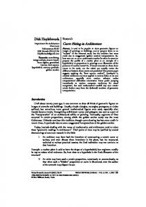
Intervvl duration (sampJinq periods) Fig. 1 A - E . Effects of discrete sampling on interval durations measured from single channel currents. A, C Selected traces of idealized (true) single channel currents which make instantaneous transitions between a shut (arrow) and open level. Currents are sampled at times indicated by filled circles. Durations of the true intervals are between 0 and 2 sampling periods in A and between t and 3 sampling periods in C. B, D Idealized measured intervals if sampled as in A and C respectively. Measured duration is given by the sampling duration times the number of samples when the interval is above the 50% threshold. E Probability that true intervals with durations between N--1 and N + 1 sampling periods are measured to have a duration of N sampling periods
matic diagrams of single channel current being sampled at a fixed sampling period of T ms. Each filled circle indicates a point in time at which the current level is sampled. These points are plotted at the 50% threshold level used for detection of opening and shutting transitions (cf. Sachs et al. 1982; Colquhoun and Sigworth 1983). If the current is above threshold at the time of a sample, then the channel is measured as open. The number of samples the current is above threshold, N, times the sampling period, T, gives the measured duration, D, of the interval: D = NT.
(1)
Figure 1 B and D plot the durations that would actually be measured for the data in A and C, respectively. The first three open intervals in Fig. 1A are not detected, as they occur between sample points. The second three open inter-
533 vals are detected, each with a measured duration of one sampling period. Thus, from Fig. 1 A and B it can be seen that undetected intervals range between 0 and 1 sampling periods in duration, and intervals measured as one sampling period in duration range between 0 and 2 sampling periods. Figure 1 C and D show that intervals measured as two sampling periods in duration range between I and 3 sampling periods. Sampling the data at discrete intervals thus combines (or bins) the data into classes of overlapping durations. Extending the analysis in Fig. 1 A - D to the general case of intervals of all durations, indicates that intervals measured with a duration of N sampling periods range between N 1 and N + i sampling periods in duration. Figure 1 E plots the probability that an interval with a duration between N - 1 and N 4- I sampling periods will be measured with a duration of N sampling periods. The probability increases linearly from 0 to 1 as interval duration increases from N 1 to N sampling periods, and then decreases linearly to 0 as interval duration increases to N + 1 sampling periods (Sine and Steinbach 1986). In order to determine the effect of discrete sampling on the measurement of interval durations from a distribution described by a single exponential, we simulated the sampling process shown in Fig. I for two different sampling rates. The continuous lines, which are identical in Fig. 2A and B, plot the exponential distributions of true intervals before sampling. Figure 2A presents a histogram of measured intervals when the sampling period is equal to the time constant of the exponential distribution. Figure 2B presents similar data when the sampling period is 20% of the time constant. The measured duration of each of the true open intervals was determined, as in Fig. 1, by counting the number of samples occurring during each interval. The number of intervals of each measured duration was then plotted as a histogram bar one sampling period wide centered at the measured duration. When the sampling period was equal to the time constant of decay (Fig. 2A), the measured number of intervals in each bin (YI) was greater than those (Y2) in a bin of equal width with magnitude equal to the magnitude of the exponential describing the true intervals at the midtime of the bin. The measured number of intervals is greater since the frequency of occurrence of true intervals falls exponentially with duration, and the durations of the true intervals combined into each histogram bin range over two sampling perdiods (Fig. 1 E). The sampled data are thus promoted in amplitude (Sine and Steinbach 1986). This promotion will be defined as
YI Ps-
Y2
magnitude of sampling bin N magnitude of true exponential at midtime of sampling bin N
(2) where Ps is the promotion ratio due to sampling, and Y1 and Y2 are as indicated in Fig. 2A. Since the sampling promotion ratio is the same for each bin (see following section), the magnitude of each bin is increased by a constant fraction and the time constant of decay of the sampled data remains unchanged (Sine and Steinbach 1986). The sampling promotion ratio for Fig. 2A, where the sampling period equals the time constant, is 1.08616. When the sampling
~oooo~ A c
8000]~
@ C O
6000-'~ E
L Q/ Q-
> k~
4000-
/u
Y~
20000
2
3
4
5
IntervoldurotJon (timeconstonts)
~ooo-
B
16oo
N
u~
OH . . . . . . . . . . . . . . . ,. , 0 1 2
,
3
, 4
Intmcvoldurotion(timeconstonts) Fig. 2A, B. Discrete sampling increases bin amplitudes of data derived from an exponential distribution of interval durations. A Histogram of measured interval durations when the sampling period is equal to the time constant of the true intervals (A) or to one fifth the time constant of the true intervals (B). I11/II2is the sampling promotion ratio as defined by Eqs. (2) and (7). Y1 and Y2 are not plotted in B because their values are nearly identical when the sampling period is small compared to the time constant. Intervals were generated and sampled by computer as described in Methods
period was 20% of the time constant of decay, as in Fig. 2B, the magnitude of each bin was only just perceptively higher (sampling promotion ratio of 1.0033) than the amplitude (at the bin midtimes) of the exponential describing the true intervals. Figure 3 plots the sampling promotion ratio as a function of the sampling period, expressed in units of time constant. The error introduced by sampling was large when the sampling period exceeded the time constant of decay of the distribution of true intervals. Decreasing the sampling period decreased the error. When the sampling period was less than 20% of the time constant of the distribution, then the sampling promotion error became small enough to introduce negligible error in the measured number of intervals.
(b) Calculation of the sampling promotion ratio. Since it is not always practical to sample the data at the necessary high
534 2.0'
~
.2
~1.8.
1.D
ca_ .~ 0.8
L
~1.6' ~
~
4.
O, 6-
a-D 4
~1.2. to
~/gl
g
-'~
J
1.0
// |
>ooe Somplin~ poriod
rate to reduce sampling promotion error to small values, it would be useful to correct for the promotion in amplitudes due to sampling. This section presents expressions to calculate the sampling promotion ratio directly, rather than by simulating the sampling process. The continuous line in Fig. 4 plots the exponential distribution of all true intervals between N - I and N + 1 sampling periods for a distribution in which the time constant equals one sampling period. The dashed line plots the number o f true intervals with a measured duration o f N sampling periods. The dashed line was calculated at each point in time from the probability that a true interval of indicated duration will be measured with a duration of N sampling periods (Fig. 1 E) times the number of true intervals of each indicated duration (exponential continuous line). The area under the dashed line reflects the number of intervals with a measured duration of N sampling periods, expressed as a fraction of all the intervals in the distribution. During data analysis this fraction would be plotted, as in Fig. 4, as a histogram bar centered at N with a width of one sampling period and an area identical to that under the dashed line. A (N), the fraction of all true intervals that are measured to have a duration of N sampling periods (the area under the dashed line in Fig. 4) is, from Sine and Steinbach (1986), NT
~
tau -2 T - l [ t - ( N -
(3)
(N + 1)T
~
t a u - 2 T - 2 [(N + 1) T - t]e -t/tau dt
t=NT
where T is the duration of a sampling period, tau is the time constant of decay of the exponential, and N >_ 1 in this and the following equations. Evaluation gives, A (N) = tau T-2 e-(N - 2)r/tau ( 1
--
e-T/tau)2
.
a:OJ
O
N-I
N
Intorvol durotion (somp/Jn~
(4)
Dividing the fractional area, A (N), by the bin width, T, gives M(N), the magnitude o f a bin centered at N with width T M(N) = tau T -2 e -(N - 2) T/tau (1 -- e - T/tau)2 (5) where magnitude is expressed as events per bin width of time.
N+I
periods)
Fig. 4. Method used to calculate the effect of discrete sampling on measured interval durations. The continuous line plots the exponential distribution of true intervals with durations from N - 1 to N + 1 sampling periods. The dashed line plots the relative number of these true intervals that are measured by sampling to have a duration of N sampling periods. The dashed line is the product of the number of true events (exponentially decaying line) times the probability that an interval will be measured as N sampling periods (Fig. 1 E). The area under the dashed line gives the fraction of all events in the true distributions that are measured by sampling to have a duration of N sampling periods. These events are plotted as an histogram bar centered at N with amplitude Y1. The dotted line, I12, is the amplitude of the distribution of true intervals at time NT, the midtime of bin N. Y1/Y2 is the sampling promotion ratio. I13 is the amplitude of an histogram bar with a width of one sampling period and an area equal to the area under the distribution of true intervals between N and N + t sampling periods. Y1/Y3 is the sampling promotion ratio of Sine and Steinbach (1986)
The magnitude, MD (N), at the midtime of the bin centered at N of the exponential describing the distribution of true intervals is M D ( N ) = t a u - 2 e-NT/tau.
(6)
Substituting Eqs. (5) and (6) into Eq. (2) to determine the sampling promotion ratio, Ps, gives P~ = tau 2 T - z (e r/t"" + e - r/tau - 2).
1)7]e-t/t""dt
t=(N-1)T
+
" . ~
(units of tJm~ constont)
Fig. 3. The sampling promotion ratio increases as the sampling period increases relative to the time constant of the true intervals. The sampling promotion ratio was calculated from YI/Y2, as defined in Fig. 2, for different sampling rates
A(N) =
Y2
(7)
Equation (7) was found to describe the promotion in magnitude of histogram bars over the exponential distribution o f true intervals at the bin midtimes for data sampled by simulating the sampling process, as described for Figs. 1 - 3. Our definition of the sampling promotion ratio differs from that of Sine and Steinbach (1986). We calculate the promotion o f the magnitude of the histogram bar N over the magnitude of the true exponential distribution at the midtime of bin N, whereas Sine and Steinbach (1986) calculate the promotion of the area of histogram bar N over the area under the true exponential distribution between N and N + 1. Each method is internally consistent and either could be used to correct for errors introduced by sampling as long as the definitions are taken into account. The magnitude o f the sampling promotion error appears considerably greater for the definition of Sine and Steinbach (1986) because the comparison of sampled intervals is made
535 to true intervals of longer durations where the frequency of occurrence is less. For example, when the sampling period is equal to the time constant, the sampling promotion ratio from the definition of Sine and Steinbach (1986) is 1.72 (ratio of Y1 to Y3 in Fig. 4) compared to our sampling promotion ratio of 1.086 (ratio of Y1 to Y2 in Fig. 4) given by Eq. (7). We have chosen to define the sampling promotion ratio with Eqs. (2) and (7) as these equations are immediately applicable to correcting sampling promotion errors with least squares and maximum likelihood fitting procedures (see below). Our definition of the sampling promotion ratio also allows easy visual judgement of possible sampling promotion errors. If the exponential describing the true intervals is equal to the magnitudes of the histogram bars of sampled data at their midtimes, then there is no error.
(2) Fitting distributions of sampled interval durations Kinetic schemes and rate constants can be estimated from the distributions of open and shut interval durations using iterative procedures (cf. Colquhoun and Hawkes 1981, 1982; Magleby and Pallotta 1983; Roux and Sauve 1985; Wilson and Brown 1985; Blatz and Magleby 1986a, b). Least squares and maximum likelihood fitting methods (discussed in Colquhoun and Sigworth 1983) are often used to assess the fit with each iteration. Least squares minimizes the sum of the squared errors (or differences) between the experimental and predicted distributions. Maximum likelihood maximizes the probability that the data are drawn from the predicted distribution. Maximum likelihood has an advantage of providing a more rational basis for weighting the different experimental points and for comparison of results between experiments Colquhoun and Sigworth 1983; Horn and Lange 1983). Since the predicted distributions for many kinetic schemes are sums of exponentials (Colquhoun and Hawkes 1981) or approximated by sums of exponentials when the data are collected under conditions of limited time resolution (Blatz and Magleby 1986a), then the fitting problem is to determine the time constants and areas (or magnitudes) of the exponential components which sum to make the distribution of interval durations.
(a) Least squares fitting with correction for sampling promotion error. Figures 2 - 4 suggest that significant errors can arise in estimates of the exponential components due to sampling promotion errors if the sampling period is greater than 20% of the fastest time constant in the distribution of true intervals. Fitting an exponential to sampled data with least squares will give the correct time constant, but the magnitude of the fitted exponential will be increased over that of the true exponential by the sampling promotion ratio. The true magnitude is then determined from the fitted magnitude with
determined with Eq. (8) by dividing the observed intercept of sampled data by the sampling promotion ratio calculated with Eq. (7). If the distribution to be fit consists of more than one exponential, as is typically the case since channels usually have multiple open and shut states (cf. Colquhoun and Hawkes 1981; Magleby and Pallotta 1983; Colquhoun and Sakmann 1985; Kerry et al. 1986), then it is necessary to correct each exponential component. For least squares fitting of multiple exponentials the magnitudes and time constants of the sampled data are first determined by fitting the sampled data. The promotion ratio is then determined for each component with Eq. (7), and the true magnitude of each components calculated with Eq. (8).
(b) Maximum likelihood fitting of data without sampling promotion error. Colquhoun and Sigworth (1983) have described maximum likelihood fitting in detail. This section briefly summarizes the method of maximum likelihood fitting for data without sampling promotion errors to lay the groundwork for the following section which indicates what modifications are necessary to determine true parameters from sampled data. We have adopted the terminology and equations of Colquhoun and Sigworth (1983) for ease of comparison between the methods. The parameters to be estimated are the time constants and areas of the exponential components which sum to form the true distribution of interval durations. This distribution, f(t), is described by k
f(t) = ~ ajtauj-le -m"uj
(8)
where Magtr~ is the magnitude of the exponential describing the true interval durations in the absence of sampling promotion error and Magobs is the magnitude determined from fitting the sampled data by least squares. For example, using least squares to fit the logarithm of the amplitudes of histogram bins 1 - 5 in Fig. 2A using the midtimes of the bins for the time values gave the correct slope of - 1.00 (time constant of 1.0 sampling period) and an intercept for the sampled data of 10,860. The true intercept of 10,000 is then
(9)
where al through ak are the areas of the k exponential components in the distribution, and taul through tauk are the time constants of the components. If no intervals with durations less than a specified duration, train, or greater than a specified duration, tmax, are detected because of experimental limitations, then the probability (density) that an interval is drawn from the true distribution, assuming no error from discrete sampling of data, is k
Y~ a~ tau)- a e - t/tau~
f(t) -- j=l
P (tmin < t < /max)
tmin < t < /max
(10)
where the denominator is the probability that an observed interval drawn from the distribution described by Eq. (9) lies between tmi, and tm,x- The denominator, assuming no sampling promotion error, is given by P ( t m i n < t < tmax) =
Magtru~ = Magobs/Ps
0 < t < oo
j=l
k ~, a j ( e -tmi"/taui - - e-tmax/tauj). j=l
(11)
For a trial set of values of the parameters (areas and time constants), the probability that each observed interval duration is drawn from the distribution described by Eq. (9) is calculated with Eqs. (10) and (11). The logarithms of the probabilities for each interval are then added to obtain the log likelihood estimate, L (0), for the trial parameters. This entire process is repeated using a search routine, such as Patternsearch (Colquhoun 1971), until parameters which maximize L (0) are found.
536
(c) Maximum likelihood fitting with correction for sampling promotion error. Maximum likelihood fitting can be developed to correct for sampling promotion error in sampled data by using an approach similar to that described in the previous section to calculate the probability that sampled intervals are drawn from the true distribution described by Eq. (9). Figures 1, 2 and 4 show that sampling combines the true intervals into bins. The measured durations of intervals in a single bin are all identical, but the true durations range over two sampling periods. For maximum likelihood fitting, then, it is necessary to know the average probability that an interval in a designated bin is drawn from the true distribution. If it is assumed, for the moment, that the denominator in Eq. (10) is 1 for sampled data (which is not the case), then it is a simple matter to calculate this probability by use of the sampling promotion ratio. From Fig. 4 and Eqs. ( 2 ) - ( 5 ) it can be seen that M(N), the numerator of the sampling promotion ratio is simply the average probability that an observed interval of N measured sampling periods in duration is drawn from a true distribution with time constant tau. This is the case since the area under the dashed line in Fig. 4, which determines the area of the histogram bar centered at N, is the sum of the probabilities that the measured intervals in bin N are drawn from a true distribution with time constant tau. Dividing this summed probability by the sampling period to determine the magnitude of the histogram bar then gives the average probability and numerator, M(N). The denominator of the sampling promotion ratio, Mo(N), is the probability that a true interval of exactly N sampling periods in duration is drawn from the same true distribution. Thus, the sampling promotion ratio, P~, gives the promotion in probability of a sampled interval over a true interval of equal duration. Therefore, the probability, P(N), that a sampled interval with a measured duration of N sampling periods is drawn from the true distribution is simply the promotion in probability, P , times the probability that a true interval of equal duration is drawn from the same true distribution: P(N) = P~ tau- 1 e--NT/tau. (12) When the true distribution is the sum of k exponentials, then k
P(N) = ~, P~jajtau]-~ e -NT/t"j
(13)
j=l
where P~j is the sampling promotion ratio for component j calculated with Eq. (7), time constant tauj, and sampling period T. The denominator to replace Eq. (11) for maximum likelihood fitting of sampled data is the probability that the intervals in the bins to be included in the fit are drawn from the true distribution. For a single exponential distribution this is simply the sum of the fractional areas of all the sampling bins included in the fit. Equation (4) gives the fractional area for a single sampling bin. Thus, the area, PD, expressed as a fraction of the total area, for bins ranging from
Nml n to Nma x is Nmax
PD =
~
tauT-le-(N-X)T/tau(1
-- e-T/tau) 2
(14)
N = Nmiz
where Nml, and Nm,~ are the minimum and maximum sampling bins to be included in the fit. The durations of observed
intervals to be included in the fit thus range from Nmi. to Nm~x sampling periods in duration. Noting that PD is the sum of a geometric progression from Nmin to Nm~x, the solution to Eq. (14) becomes PD = tau T - ~ (e - ( N ~ - 1)T/tau __ e - N m i n r / t a u --
e- N m a x T / t a u
~_ e - (Nmax + 1)T/tan) .
(15)
When the distribution of true intervals is composed of the sum of exponentials, the probability, PD, that an interval with the distribution of Eq. (9) has a measured duration within Nmln to Nm~xsampling periods, inclusive, is k
PD = ~ aitauj T -1
(e -(Nmin-1)T/tauj
- - e -Nm~nT/tauj
j=l
_ e-Nma.T/t~uj + e-(Nm.~+1)T/t.u0.
(16)
L(0), the logarithm of the likelihood that sampled intervals from Nm~. to Nm.x, inclusive, are drawn from the true distribution described by Eq. (9), is obtained by summing the logarithms of the probabilities over the bins of sampled intervals to obtain, k
N~
L(0)=
~
~ P~ajtauf 1e-NT/tauj
r(U)log .~:~
N = Nmirt
PD
(17)
where Y(N) is the number of intervals in bin N, PD is given by Eq. (16), P~j is given by Eq. (7), and the summation expression in the numerator is from Eq. (13). The summation expression divided by the denominator gives the probability that a single observed interval with a measured duration of N sampling periods is drawn from the true distribution described by Eq. (9). The logarithm of this value times the number of intervals in bin N gives the logarithm of the probability that all the intervals in bin N are drawn from the true distribution. The sum of the logarithms of the probabilities for bins Nmi~ to Nm~xgives L(O), the logarithm of the probability that all intervals in bins Nmi, through Nmax are from the true distribution. As with non-sampled data, a search routine is then used to repeat this process to find the areas and time constants which maximize the log-likelihood estimate, L(O). The determined parameters and Eq. (9) then describe the most likely true distribution of intervals for a given number, k, of exponential components. There are only 2 k - 1 free parameters as the areas must sum to 1. Repeating this process for different numbers of exponential components and application of the likelihood ratio test (Rao 1973; Horn and Lange 1983) then allows deterlnination of the minimum number of significant exponential components. Once the most likely number of exponential components and parameters are found, an estimate of Aft.... the true number of intervals in the true distribution is obtained from Ntrue =
Nnb~/PD
(18)
where Nob~is the sum of the number of intervals in sampling bins N~i~ through Nmax, and PD is given by Eq. (16). Equation (17) was tested by fitting sampled intervals drawn from true distributions of one or more summed exponentials. In all cases examined, including those in which the sampling interval was twice the duration of the fastest time constant of decay in the data, the values of the parameters that maximized the log-likelihood value L(O) were essentially identical to the true parameters described the
537 initial distribution. For example, maximum likelihood estimates of the true parameters obtained by fitting the sampled data in bins 1 - 5 of Fig. 2A were 10,000 true intervals with a time constant of 1.0000 unit, the same as the true parameters, As Eqs. (16) and (17) are easily applied, they provide a simple method for correction of sampling promotion error. If correction for sampling promotion error was not applied during maximum likelihood fitting, then significant errors in estimation of the time constants occurred if the sampling period was greater than about 1 0 - 2 0 % of the fastest time constant. Without correction during maximum likelihood fitting, time constants were usually overestimated by an amount similar to the sampling promotion error, with the actual error depending on the minimum and maximum times used in the fitting. When sampled data consisting of sums of exponentials were fit without correcting for sampling promotion error, the maximum errors were considerably worse than these, as small errors in the faster decaying components with a large fraction of the total area could give rise to much larger errors (up to several hundred percent) in estimates of the areas of the slower decaying components which contained only a small fraction of the total area.
(3) Effect of combining data into bins Since large numbers of intervals are necessary to detect exponential components with small areas, or to resolve components that have time constants that are not widely separated, it would be advantageous to combine some of the data into bins larger than the sampling period to decrease the number of steps required to fit the data, if this could be done without error. For example, if, in a particular experiment, 100 intervals occur with durations between 95 and 105 ms, combining these intervals into a single bin with a mean duration of 100 ms, a width of 10 ms, and a magnitude of 100 would reduce by a factor of about 100 the number of steps required to fit these intervals. Also, it is necessary to combine data into bins for meaningful plots, as there are seldom enough intervals of longer durations for plots of data at the resolution of the sampling period. This section of the paper assess errors arising from combining intervals into bins for the conditions of either measuring interval durations with continuous time resolution or measuring by sampling.
(a) Binning promotion ratio for intervals measured with continuous time resolution. Figure 5 shows potential errors associated with binning intervals measured with continuous time resolution. The continuous line plots the exponential distribution of true intervals to be binned. The data are combined into bins with a width B and centered at times of 1, 2 . . . . n bin widths. Thus, intervals with duration ( n 0.5) B to (n + 0.5)B are combined into bin n centered at time n B. The shaded area, which represents the fraction of all intervals combined into bin n, is given by B(n+0.5)
Areatrue =
~
t a u - 1 e-t/tau dt
t =B(n-0.5)
where B is bin width and tau is the time constant of the true intervals. Integration gives Areatrue
=
e -nB/tau ( e 0 " S B / t a u - - e - O ' S B / t a u ) .
"~, 13.8 c iS 06 .l.a
c >~ 13.4 O
.~ ~d 13.2 0 n-I Interval
i
i
n
n+1
durotion
(bin widths)
Fig. 5. Effect of binning exponentially distributed interval durations. The continuous line plots an exponential distribution of true intervals with durations from n - l to n + 1 bin widths and time constant of one bin width. If all the true intervals with durations from (n--0.5)B and (n + 0.5)B (shaded area) are combined and plotted as a histogram bar centered at n with a bin width of b, then the amplitude of the histogram bar is Y4. Y5 is the magnitude of the true distribution at n, the bin midpoint. The binning promotion ratio is defined as Y4/Y5 and by Eq. (22)
Plotting the shaded area as a bin centered at n with B units of width gives a magnitude, MB, of M B = B - 1 e-nB/tau (eO.5B/tau _ e- 0.sB/tau) (19) indicated by Y4 in Fig. 5. Defining the binning promotion ratio, Ps, as the magnitude, Y4, of the bin centered at n divided by Y5, the magnitude of the exponential describing the true intervals at time Bn gives Y4 PB = Y5
MR t a u - 1 e-nB/tau
which when combined with Eq. (19) reduces to PB = t a u B - 1 (e0.5B/tau _ e-0.SB/tau).
(20)
(21)
For the example in Fig. 5, where the bin width and time constant are equal, the binning promotion ratio is 1.0422. This can be compared to 1.0862 for the sampling promotion ratio for the same conditions. The error is less for the binning promotion ratio because intervals within a single bin have true durations lying within the width of the bin, whereas intervals in a sampled bin include true durations from outside of the plotted width of the bin, as indicated in Figs. 4 and 5. From Eqs. (21) and (7) it can be shown that the binning promotion ratio is equal to the square root of the sampling promotion ratio. Figure 6 plots the binning promotion ratio against the bin width, expressed in units of the time constant of the binned intervals. The binning error only becomes significant as the bin width exceeds 30% of the time constant. For example, for bin widths of 10%, 20%, 30% and 50% of the time constant, the binning promotion ratios are 1.00042, 1.0017, 1.0038, and 1.0104, respectively. Thus, binning should introduce little error if the bin width is less than about 20% of the fastest time constant in the original data.
538 NL
1.5-
A (0) e- ur/ta, o ~
1.4-
9~
1,9"
Mm-
W
L ~1.2"
.E 1.1. 1.0
N=NF
J
Bin width (units os time constont)
Fig. 6. The binning promotion ratio increases as bin width increases relative to the time constant of the true intervals. The binning promotion ratio, defined as Y4/Y5 in Fig. 5 was calculated with Eq. (22)
where MB~ is the magnitude of the bin which combines sampling bins with measured durations of NF to NL sampling periods, T is the duration of the sampling period, tau is the time constant of the distribution of true intervals, A(O) is the magnitude of the distribution of true intervals at time zero, and A(O)e -NT/tau is the corrected magnitude of sampling bin N after dividing the observed magnitude by the sampling promotion ratio. Noting that the numerator is the sum of a geometric progression gives (1 -
r w) A(0) e - N F r / ' "
(1 - - r) M a s --
W
Y ~ e-T/tau
(b) Binning promotion ratio for intervals measured by sampling. When intervals measured by sampling are combined into bins of duration greater than the sampling period, then there is a binning promotion error in addition to the sampling promotion error. The calculation of the binning promotion ratio for sampled data must take into account the fact that sampling itself combines data into bins (sampling bins) of plotted width equal to the sampling period. This can be seen by considering Fig. 2A. The magnitudes of the sampling bins containing intervals with sampled durations of 1, 2, and 3 time constants are 3,995, 1,470, and 541 intervals, respectively (YI). The corrected magnitudes of these sampling bins after dividing by the sampling promotion ratio of 1.086 [Eqs. (7 and 8)], are 3,679, 1,353, and 498 intervals, respectively (Y2). If the three corrected sampling bins are then combined into a single bin, the combined bin would have a width of three time constants equal to the width of the three sampling bins. The center of the combined bin would be at two time constants, and the magnitude of the combined bin would be given by the number of intervals in the three combined corrected sampling bins divided by the width of the combined bin: (3,679 + 1,353 + 498)/3 = 1,843. The magnitude of the exponential describing the continuous distribution of true intervals (continuous line) at the midtime of the combined bin is: 10,000 e x p ( - 2 / l ) = 1,353. Defining the binning promotion ratio for sampled data as the magnitude of the combined bin divided by the magnitude of the true distribution of intervals at the midtime of the combined bin gives: 1,843/1,353 = 1.36. Thus, the magnitude of the combined bin with correction of the sampling bins for sampling promotion error is 36% higher than the exponential describing the distribution of true intervals at the midpoint of the combined bin. The process of determining the binning promotion ratio for sampled data may be formalized as W = (NL-- NF + 1) where W is the number of sampling bins combined into one bin, and NF and NL are the durations in integral sampling periods of the first and last sampling bins in the combined bin.
where r is the common ratio between the magnitudes of successive sampling bins; that is, r is the ratio between the number of intervals with measured durations of (N + 1) and N sampling periods. Finally, MBs PBs = A (0) e- 0,5 T(NL + NF)/tau
(22)
where PBs, the binning promotion ratio for sampled data, is given by MB~, the magnitude of the bin which combines the corrected sampling bins, divided by the magnitude of the exponential describing the distribution of true intervals at the midpoint of the combined bin. Notice that A(0) in the expression for M~ will cancel A (0) in the denominator of Eq. (22). For the example considered previously is which the combined bin width is equal to three time constants of the distribution of true intervals, Eq. (22) gives binning promotion ratios for sampled data of 1.0, 1.29, 1.36, and 1.41 for sampling periods equal to 100%, 50%, 33.3% and 10% of the combined bin width, respectively. In the limit of vanishingly small sampling periods, Eq. (22) for sampled data gives, as expected, the same binning promotion ratio of 1.42 as Eq. (21) for continuous data. Calculations of this type indicated that the binning promotion ratio for sampled data is similar to the binning promotion ratio for intervals measured with continuous time resolution, as plotted in Fig. 6, if the sampling period is less than about 10% of the bin width. For larger sampling periods, the binning promotion ratio for sampled data is less than for continuous data, and may be calculated with Eq. (22).
(c) Least squares fitting with correction of binning promotion error. To correct for binning promotion error with least squares fitting of intervals measured with continuous time resolution, Ps in Eq. (8) is replaced with the binning promotion ratio, PB, calculated with Eq. (21). When least squares fitting is used to fit sampled intervals combined into bins, it is necessary to correct for both sampling and binning promotion errors. Equation (8) already makes the correction for sampling promotion error for least squares fitting. The additional correction required for combining sampled data into bins is made by multiplying Ps in Eq. (8) by Pro, calculated with Eq. (22). Each fitted corn-
539 ponent is corrected separately if the data consist of sums of exponentials.
bin = 1 + integer IRes • loglo (duration of interval in sampling periods)]
(d) Maximum likelihood fitting with correction for binning promotion error. To correct fbr binning promotion error
where Res is the resolution factor which sets the number of bins per log unit. When Res is 100, then there are 100 bins per log unit and the bin width averages 2.3% of the bin midtime. Decreasing Res to 50 or 25 gives 50 or 25 bins per log unit, respectively, with bin widths of 4.6% or 9.3% of the bin midtimes, respectively. Average bin width is calculated from, 10 (~/{R~ + ~)) - 1. Notice that duration is always expressed as an integral number of sampling periods. To estimate the potential binning error for a resolution of 100, consider an exponential component with a time constant of 1 unit. Since bin width increases with the duration of intervals, then an estimate of the maximum binning error can be obtained by determining the binning error for the longest duration intervals likely to be observed. Less than one interval per thousand will exceed seven time constants in duration. The bin width for an interval seven time constants in duration will be seven times 0.023, or 16% of the time constant of decay. The binning promotion ratio associated with a bin width of 16% the time constant of decay is 1.0011, a negligible increase. Since binning errors would be less than this low level for 99.9% of the intervals, the binning error associated with a resolution of 100 is insignificant. Similar calculations show that the binning error only becomes significant for resolutions of less than about 25 bins per log unit. For a resolution of 100 bins per log unit, intervals of 1, 10, 100, 1000, and 10 l~ sampling periods in duration are placed in bins 1, 101,201,301, and 1001, respectively with Eqn. (23). Consequently, an array of only 1001 bins is sufficient to store, with negligible error, intervals whose duration range over ten orders of magnitude. I f the sampling period is 1 gs, then intervals with durations from 1 gs to 2.7 h can be accomodated for a resolution of 100. If the resolution is 25, the same array could bin intervals from 1 ps to the age of the universe with insignificant error. For most biological applications, a resolution of 25 and a few hundred bins would be sufficient.
during maximum likelihood fitting of intervals combined into bins, the summation, N = Nmin to Nmax, in Eq. (17) is replaced by: N" = N'ml, to Nm,x, where N~i, to N'm,x serves as a counter to step through the combined bins: N'~n is the first combined bin included in the fit, and Nm~x is the last combined bin included in the fit. Y(N) is replaced with Y(N'), where Y(N') is the absolute number of intervals in each combined bin. Finally, NT is replaced by t(N'), where t(N') is the midtime duration of each combined bin. If the interval durations combined into bins are measured with continuous time resolution, then Psi in Eq. (17) is replaced with PBi(N'), calculated for each combined bin N' and componentj with Eq. (21) using the width of combined bin N' and the time constant of component j, and PD in Eqs. (17) and (18) is calculated with Eq. (11). PBi(Nt) then corrects for the promotion in amplitude when intervals measured with continuous time resolution are combined into bins. If the interval durations combined into bins are measured by sampling, then it is necessary to correct for both sampling and binning promotion errors. Equations (17) and (18) already correct for sampling promotion error. The additional correction required for combining sampled intervals into bins is made by multiplying Ps~ in Eq. (17) by PBsj(N'), calculated for each combined bin N' and component j with Eqn. (22) using the width of combined bin N' and the time constant of component j. Psj corrects for the sampling promotion error. Multiplying Psi by PB~(N') then corrects for combining sampled intervals into bins. PD in Eqs. (17) and (18) for sampled intervals combined into bins is calculated with Eq. (16) where Nm~, and Nm,x are the first and last sampling bins included in the fit.
(4) Log binning, plotting and fitting interval durations The durations of intervals recorded from a single channel often range over many orders of magnitude (cf. Blatz and Magleby 1986b). In order to detect an exponential component, it is necessary to obtain data from that component at several different points in time. If bin width is chosen to detect the fastest decay components in the data, then the number of bins required to bin intervals of all durations becomes unmanageable, and the bin width is too narrow to effectively combine intervals of long durations. If the bin width is increased, then the fasted decaying components may be missed, and large binning errors can result for intervals of brief durations. This section presents a method to bin and plot distributions of interval durations which overcomes these problems. Intervals are binned according to the logarithms of their durations and a resolution factor. Such a procedure leads to an increase in bin width as interval duration increase, but keeps a relatively constant relationship between bin width and bin midtime. Consequently, components of all time courses can be detected. I f bin width is selected to be less than about 20% of bin midtime, then there is essentially no binning error, as each component decays to negligible levels before bin width exceeds 20% of the time constant of that component.
(a) Log binning. The data are binned according to
(23)
(b) Decoding log binned data. Because of the log binning and the necessary integer operation to determine a bin, the midtime of a bin is only approximated by solving for duration in Eq. (23), and bin width varies in a complex and nonmonotonic manner with bin number. In order to decode the binned data, an additional file is created which stores for each bin the actual midtime of the bin and bin width. These times are stored in terms of sampling periods. Consequently, for a given resolution, one decoding file is sufficient for data measured with any sampling period. The decoding file is made by using Eq. (23) to bin all integral numbers between 1 and 10 ~~ and tabulating the number of intervals and the mean duration of the intervals that fall in each bin. The width of each bin in units of sampling periods is given by the number of intervals that are binned in that bin. The midtime of each bin is given by the mean duration of all intervals that fall in that bin. For example, for a resolution of 100 the midtime and bin width for bin 1 are both 1 sampling period. For bin 169 the midtime and bin width are 48 and 1 sampling periods, respectively; for bin 170 the midtime and bin width are 49.5 and 2 sampling periods, respectively; and for bin 500 the midtime and bin width are 98861.5 and 2276 sampling periods, respec-
540 tively. The decoding file should be made using the same programming language, level of precision for the logarithm (single or double), and machine hardware as will be used to bin the data so that the decoding file is an exact match to the binned data. A difference in the sixth place of a logarithm arising from differences in precision or machine hardware can change the integer value of some numbers and hence the bins that intervals are plotted in. After interval durations, expressed in integral numbers of sampling periods, are binned with Eq. (23), the midtime and bin width of each bin, expressed in sampling periods, are read from the decoding file, converted to time with Eq. (1), and stored with the number of events in each bin.
10000-~ 1000E CO C~
d
~
100" 10- . . . . . . . . . . . . .
-'~-
1 i-
( c) Plotting log binned data. The plotted number of intervals in each bin AT' is scaled for bin width with NUmplot(N') = number of intervals in bin N'/width of bin N' (24) where NUmplot(N') is magnitude of bin AT' to be used for plotting. The plotted bins are centered on their midtimes, determined previously from the decoding file and Eq. (1). With resolutions of 5 0 - 1 0 0 bins per log unit, the bins at longer times will most likely not contain a sufficient number of intervals for effective plotting, unless the sample size is large. Consequently, for plotting the data can be rebinned at a larger relative bin width using resolutions of 5 - 2 5 bins per log unit, or two or more adjacent bins in the high resolution data can be combined before plotting.
(d) Least squares fitting of l o g binned data. The magnitudes used for least squares fitting of log binned data are the magnitudes of each plotted bin, Nvlot(N'), given by Eq. (24). Corrections can be made for sampling promotion error, if the data are sampled, with Eq. (8) after fitting. A resolution of 25 or more bins per log unit avoids binning promotion error, which cannot be corrected for with least squares fitting by the method described in Part I, sect. 3c, because of the increasing bin size. (e) Maximum likelihoodfitting of log binned data. Maximum likelihood fitting of log binned data is the same as maximum likelihood fitting of binned data described in Part I, sect. 3d. The increasing bin width for log binned data is accounted for automatically during the fitting, as PBj(N') for continuous data, or P~j(N') for sampled data, is calculated with Eq. (21) or (22), respectively, for each combined bin N' based on the width of the combined bin. For fitting of sampled data the values of Nm~, and Nm~x used in Eq. (16) for the minimum and maximum interval durations expressed as N sampling periods can be obtained from the decoded file, which stores durations in time rather than sampling periods, with N~m Nmi
n
=
Nm,x =
0.5(N~w - 73 T
(25a)
N'Lm + 0.5(N[, -- 73 T
(25b)
-
-
where N'Fmand N[m are the midtimes and N~w and N[w are the widths of the first and last bins, respectively, of the log binned data to be included in the fit, and T is the duration of the sampling period used in the initial analysis of the data.
>
0.1
0.01 O.001 0.01
\\/ i
i
i
O. I
i
I0
i
100
Int~rvoldurotJon(ms) Fig. 7. Binning intervals based on the logarithms of their durations provides an efficient means of data handling. The continuous curve plots, on log-log coordinates, a distribution of true interval durations consisting of the sum of four exponential components with time constants of 0.05, 0.25, 1.25, and 6.25 ms and relative areas of 0.8000, 0.1600, 0.0320 and 0.0064, respectively. 104,280 intervals from this true distribution were measured with a sampling period of 0.005 ms, binned at a resolution of 100 bins per log unit with Eq. (23), decoded, and plotted with Eq. (24). The results are shown by the stepwise line evident in the enlargements, where each step represents the top of a histogram bar. The true distribution (curve) passes through the center of each of the bins. The dashed lines plot separately the four exponential components which sum to form the true distribution.
For fitting of intervals measured with continuous time resolution, bin width and midtimes can be calculated directly, rather than with a decoding file, but decoding files are still useful to prevent repeating these calculations each time data is binned. In order to use the same programs for continuous data as used for sampled data, the duration of intervals measured with continuous time resolution can be expressed in terms of sampling periods, where the sampling period used with Eq. (23) is sufficiently small, such as 0.001 ms, so that the desired time resolution is maintained, and the calculated correction for sampling promotion error is negligible.
(f) Plotting with log - log coordinates and estimates of error associated with fitting sampled and log binned data. Figure 7 shows that log binning and decoding introduces insignificant error. The continuous line represents a distribution of intervals described by the sum of four exponential components with time constants of 0.05, 0.25, 1.25 and 6.25 ms and relative areas of 0.8000, 0.1600, 0.0320, 0.0064, respectively. The dashed lines represent the individual components. The data are plotted on log - log coordinates, as this is the only practical manner to present data that spans several orders of magnitude in both the number and duration of observed events. The four bumps in the line arise from the four exponential components. Intervals from the true distribution described by the continuous line were measured with a sampling period of 0.005 ms (10% of the fastest time constant),
541 log binned at a resolution of 100 bins per log unit, decoded, and plotted on the same coordinates. The stepwise line (see enlargements) represents the results obtained from analyzing 104,280 intervals from the true distribution in this manner. (The stepwise line is the top of the histogram of the binned data.) The log binned, decoded and plotted data describe the true distribution, without perceptible error, as shown in the representative enlargements at short and long times where the distribution of true intervals passes through the midtimes of the bins of the log binned and plotted data. Notice that the label for the ordinate in Fig. 7 is number of intervals per sampling period to indicate the correction of Eq. (24) for plotted amplitudes with increasing bin width. In order to determine whether the true time constants and areas could be obtained from the log binned data plotted in Fig. 7, the data were fit using the method of maximum likelihood which corrects for sampling promotion error [Eqs. (7) and (16-18)], binning promotion error (Part I, section 3d), and takes into account log binning (Part I, section 4e). Areas and time constants of the four components determined by fitting the log binned data in Fig. 7 were almost identical to the true parameters, with errors ranging from 0.001% to 0.07% (mean error of less than 0.02%). Fitting the log binned data in Fig. 7 without correction for sampling promotion error increased the mean error in estimation of the parameters from 0.02% to 0.2%, indicating that correction for sampling promotion error is useful even when the sampling period is only 10% of the fastest time constant. We further tested the log binning method on data from the same distribution of true intervals shown in Fig. 7, but with sampling periods and bin widths large enough to introduce significant sampling and binning promotion errors. As in the previous example, the data were fit using the method of maximum likelihood which corrects for sampling promotion error [Eqs.(7) and (16-18), binning promotion error (Part I, section 3d), and takes into account log binning (Part I, section 4e). When the sampling period was 0.05 ms and equal to the fastest time constant in the distribution, the average error in estimates of the true areas and time constants was less than 0.02% and the maximum error was 0.06% (6.246 ms instead of 6.250 ms). The average error was independent of bin width for resolutions of 5 to 100 bins per log unit, indicating that correction for binning promotion error was satisfactory over this range of resolutions. Similar insignificant errors were found when the sampling period was twice the fastest time constant. When correction for binning promotion error was not applied in the above example, the average error increased as the resolution for the log binning decreased, being 0.02%, 0.04%, and 0.2% for resolutions of 100, 50, and 25 bins per log unit, respectively. Decreasing the log binning resolution further gave large mean errors of 6.7% and 37% for resolutions of 10 and 5 bins per log unit, respectively. Thus, if correction is not made for binning promotion error, resolutions of 25 or more bins per log unit should be used to prevent binning promotion error. The analysis presented in Part I of this paper was carried out on ideal data in order to exclude errors arising from filtering and noise. It was assumed that open-shut transitions were instantaneous and that if, for example, shut intervals were being analyzed, then all open intervals were detected, as would be the case if the open intervals were long compared to the sampling period. Under these conditions it was found
that any errors arising from sampling, log binning, decoding, and fitting the binned data with correction for sampling and binning promotion errors were insignificant.
Part H: Effect of sampling data with limited time resolution In contrast to the ideal data used in the above examples, experimental single channel currents have reduced time resolution due to the limitations of the recording techniques and the filtering required to reduce noise to acceptable levels (Hamill et al. 1981 ; Colquhoun and Sigworth 1983). When time resolution is limited, all intervals with a true duration less than a certain time, the dead time, go undetected (Colquhoun and Sigworth 1983). Undetected intervals are not necessarily a problem in data analysis, as methods are available to account for most of their effects (Colquhoun and Sigworth 1983; Roux and Sauve 1985; Wilson and Brown 1985; Blatz and Magleby 1986a; Sine and Steinbach 1986). These methods assume that all intervals with true durations greater than the dead time are detected. This section of the paper examines the effects of sampling on filtered data. It is found that sampling filtered data can produce errors in detection of intervals and measurement of durations. Thus, sampling of filtered data can lead to errors in interpretation of results.
(1) Filtering can reduce observed amplitudes and durations of intervals Figure 8 plots ideal single channel currents that would be observed with unlimited frequency response (rectangular current steps) and the filtered responses to these ideal currents (curves). In Fig. 8 A the duration of the true interval is equal to the dead time. Consequently, the filtered response just reaches the 50% level. In Fig. 8 B and C the duration of the true interval is 1.1 dead times and the duration at the 50% level is 0.676 dead times. In D, E, and F the durations of the true intervals are 1.235, 2.0 and 4.0 dead times, and the observed durations at the 50% level are 1.0, 1.98, and 4.0 dead times. Thus, with filtering and 50% threshold detection: (a) intervals with true durations less than 1.0 dead time are below threshold for detection; (b) intervals with true durations from 1 - 2 dead times have durations at the 50% level less than the true durations; and (c) intervals with true durations greater than two dead times have durations at the 50% level equal to the true durations (Colquhoun and Sigworth 1983).
(2) Measuring interval durations by sampling filtered data Figure 8 E and F show that the durations of filtered intervals greater than two dead times are correct at the 50% threshold level. Thus, if sampling with 50% threshold detection is used to measure the durations of intervals greater than two dead times, then all the findings in Part I of this paper, which characterize errors associated with measuring durations of ideal intervals with sampling, will also apply to filtered intervals greater than two dead times. Consequently, measuring durations of intervals in filtered data with sampling will introduce an error, expressed as the sampling promotion ratio (Figs. 2--4). This error can be prevented by using sampling periods less than 1 0 - 2 0 % of the fastest time constant in the distributions of intervals or by fitting the distri-
542 B
-----1
I'D'I
I I
0.5-[......
c r
e
c i
01/ 0
2
3
4
0
I
I
I
!
I
I
I
I
2
3
4
O
1
2
3
4
o
2
!
I
4
6
8
c~ o
E
4a r ill L L
a
0
1
2
3
4
0
I
I
I
4
6
8
1
Tim~ (unite of deed tim~) Fig. 8 A - F . Effect of filtering on amplitudes, durations, and detection of true intervals. Idealized (true) single channel currents are plotted as rectangular responses starting at time 0, where time is expressed in units of dead time. The responses observed with filtering are shown as the slowly rising and falling curves. ( 0 ) on the dashed 50% threshold line indicate samples taken once every dead time. A An interval with a true duration equal to 1.0 dead time just reaches the 50% threshold level. Intervals with true durations less than 1.0 dead time are not detected. B, C Only a fraction of the intervals with true durations between 1.0 and 1.235 dead times are detected. In B and C an interval with a true duration of t.l dead times and a filtered duration at the 50% level of 0.676 dead times has a 67.6% chance of being detected when the sampling period is 1.0 dead times. The interval is not detected in B and is detected in C. D With a sampling period of one dead time all intervals with true durations of 1.235 dead times or greater are detected because the filtered duration at the 50% level is equal or greater than the sampling period. E, F Intervals with true durations greater than 2 dead times have observed durations at the 50% level equal to the true durations. Intervals with true durations from 1 - 2 dead times have observed durations at the 50% level less than the true duration
butions o f open and shut intervals with Eqs. (7) and ( 1 6 18) which take the sampling p r o m o t i o n error into account.
(3) Detection of intervals with sampling I f the d a t a in Fig. 8 is sampled with a sampling period equal to the dead time, as indicated by the dots on the dashed lines, then those intervals with filtered durations at the 50% level equal to or greater than the sampling period will always be detected, since at least one sample will be taken when the current is above the 50% level. The m i n i m u m duration o f a true interval which meets the requirement o f a filtered duration at the 50% level equal to or greater than the sampling period can be determined empirically from the filtered response (see section 3 in Methods) or estimated by Eq. (17) in Colquhoun and Sigworth (1983). Figure 8 D shows that an interval with a true d u r a t i o n o f 1.235 dead times gives a filtered duration at the 50% level o f 1.0 dead time. A l t h o u g h all intervals with true durations o f 1.235 dead times or greater are detected for a sampling period o f 1.0 dead time, only a fraction of the intervals with true durations between 1.0 and 1.235 dead times are detected, as, depending on when the intervals occur, a sample might not be taken when the current is above threshold. F o r example, b o t h Figs. 8 B and C present an interval with a true d u r a t i o n o f 1.1 dead times and a filtered duration o f 0.676 dead times. The interval in Fig. 8 B is n o t detected and the interval in Fig. 8 C is. The fraction o f intervals with true durations between 1.0 and 1.235 times that are detected depends on
the distribution o f interval durations. I f the interval durations are described by a single exponential with a time constant of 1.0 dead time, then it can be calculated that 0.67 o f the intervals with true durations between 1.0 and 1.235 dead times are detected for a sampling period o f 1.0 dead time (details o f calculation in section 4 o f Methods).
(4) Sampling detection ratio The previous section shows that some intervals greater than the dead time are not detected when sampling filtered data. In order to characterize the magnitude o f this error, a sampling detection ratio, D~, will be defined as F r a c t i o n o f true intervals detected with sampling O s =
F r a c t i o n o f true intervals with durations > dead time (26)
where Ds is calculated separately for open and shut intervals. Thus, F~ ( e -
Ds =
Td/tau
e - r~/tau + ee- Ta/tau
__
To/tau
(27)
where tau is the time constant o f the distribution o f intervals to be detected, Tc is the d u r a t i o n of a true interval that gives a filtered d u r a t i o n at the 50% level equal to the sampling period, Td is the dead time, and Fs is the fraction ofintelwals with true durations ranging from Td to Tc that is detected with sampling. All intervals > Td are detected when there is no sampling error, and all intervals > Tc are detected with
543 w h e r e F~et is the fraction of intervals detected with sampling,
1.0 O
~~J O. 9L. C cJ
"~ 4O t.l 0J
O.B-
- o 0 . 7_ t~ .,m
E ~3 tO
0.6-
0.5
o
o.'s Samp1in~ period
1.'o
1Js
a'o
(units oF dead time)
Fig. 9. Effect of sampling on detection of intervals. Each curve presents data for detected intervals from an exponential distribution with the indicated time constant, expressed in units of dead time. Increasing the sampling period and decreasing the time constant decreases the number of detected intervals, as defined by Eq. (26). (O) were calculated with Eq. (27). (+) were determined numerically by simulation of filtered and sampled data. The continuous lines were calculated with Eq. (29)
sampling error. Intervals missed solely as a consequence of sampling are drawn from those intervals with true durations between Ta and To. The denominator in Eqs. (26) and (27) is simply the fraction of intervals that would be detected from filtered data when there is no sampling error. Open and shut intervals must be treated separately with Eqs. (26) and (27), unless the time constants of the two distributions are identical. Figure 9 plots the sampling detection ratio, Ds, as a function of the sampling period for single exponential distributions of intervals with time constants ranging from 0.5 to 10 dead times. The sampling detection ratio is always 1.0 or less since the error is detection of fewer events. Increasing the sampling period or decreasing the time constant of the true intervals decreases the fraction of intervals detected. For example, when the time constant of the true intervals is equal to the dead time and the sampling period is equal to one dead time, the sampling detection ratio is 0.93. This indicates that only 93% as many intervals are detected with sampling under these conditions as would be detected if the sampling period were vanishingly small. Figure 9 also shows that detection error from sampling is small for sampling rates as slow as once per dead time if the fastest time constant in the data is 10 dead times or greater. Sampling detection error is less with longer time constants because the vast majority of events have filtered durations longer than the sampling period, and consequently, are detected. The few extra events missed due to sampling are an insignificant number of the total detected events. The fraction of intervals from a single exponential distribution with time constant tau that is detected with sampling is obtained by multiplying the fraction that would be detected in the absence of sampling error by the sampling detection ratio, Ds. Thus, Fact = D~ e- ra/tau
(28)
and Td is dead time. F~et is calculated separately for open and shut intervals, and the assumption is made for Eq. (28) that the shut (or open) intervals to be detected are separated by open (or shut) intervals of long duration. For the above example where the time constant equals the dead time, 0.368 of the true intervals have durations greater than the dead time and would be detected if there were no sampling error. Thus, 0.93 x 0.368 = 0.342 of the intervals are detected with a sampling period of one dead time. The sampling detection ratios plotted as open circles in Fig. 9 were calculated with Eq. (27) using values of Tc and Fs determined numerically, as described in section 4 of Methods. The crosses, which are in agreement with the open circles, were determined by direct simulation of a two state model in which true intervals were generated, filtered, and sampled at the indicated sampling period, as described in section 5 of Methods. The time constant of the open intervals was sufficiently long (200 dead times) that essentially all open intervals were detected. The fraction of shut intervals detected for each sampling period and shut time constant was divided by the fraction detected when the sampling period was 5% of the fastest time constant, a sampling period which gives no sampling error, to detemine the sampling detection ratio, At least 300,000 true intervals were simulated in each case. The continuous lines in Fig. 9 were calculated with the empirical equation Ds = e -(0"076 T1"932t a u - ~
(29)
where T is sampling period and tau is the time constant for the distribution of intervals being detected, expressed in units of dead time.
Part III: Effect of noise
In addition to limited time resolution, experimental single channel data differs from the ideal data shown in Fig. I in that the records are noisy. This section considers two different effects of noise on interpretation of single channel data. (1) Noise peaks can produce false events
Although it is well established that noise peaks can produce false channel events (cf. Colquhoun and Sigworth 1983), it is worthwhile to first consider this effect of noise in order to distinguish it from a different effect presented in the following section. The production of a false event by noise is shown in Fig. 10, which presents an ideal current during three channel openings in A, the filtered ideal current in B, and the filtered ideal current with increasing amounts of noise in C F. When, in the absence of channel activity, noise exceeds the 50% level for threshold detection, as occurs in Fig. 10F for event 4, then a false event due soMy to noise will be detected as a channel opening. If the magnitude of noise were even larger in F, then the noise marked by 3 would be detected as a false closing. Such false events divide true events into two parts, decreasing the mean durations of observed open and shut intervals. False events due to noise peaks exceeding the 50% level can also give rise to false distributions of brief events. I f the detailed characteristics of the noise are known, then the number of false events can be estimated as described in Colquhoun and Sigworth (1983).
544 1
I
2
I
1
i
i
1
i
2
3
4
5
6
7
I
2 ms
D
Fig. 1 0 A - E . Effect of noise on filtered data. A Idealized (true)
single channel current during three channel openings. Closed channel current indicated by the arrow. B Observed current when the ideal current in A is filtered at 3.58 kHz ( - 3 dB) to give a dead time of 0.05 ms. C - F Observed response when increasing amounts of current noise are added to the filtered response in B. The added noise, expressed as the standard deviation of the single channel amplitude, was 0.05, 0.1, 0.15, and 0.2 in C - F , respectively. Noise has two effects when data are analyzed with 50% threshold detection. Noise peaks can be detected as false events (event 4), and noise can prevent or enable detection of intervals (events 1 and 2)
A n alternative method to estimate the false event rate due to noise peaks, which does not require knowing the characteristics of the noise, is to analyze the data with the threshold detection level set at an absolute distance equal to 50% o f the single channel current amplitude, but on the side of the baseline opposite from channel opening. If 10 events are detected in 20 s of data during which the channel is closed, then the false event rate from noise peaks is 0.5 per second. For noise distributed equally above and below the baseline, the false event rate from noise peaks in the direction of channel opening would be the same. False events due to noise peaks can be reduced to acceptable levels or eliminated by sufficient filtering. (2) No&e increases the fraction o f detected events
The second effect of noise can occur at lower levels of noise than those required to produce false events from noise peaks. In Fig. 10 it can be seen that noise can enable detection of some true events that would be missed in the absence of noise (event 2) and can prevent detection of some true events that would be detected in the absence of noise (event 1). Whereas Fig. 10 shows noise preventing the detection of a shut interval and enabling the detection of an open interval, noise can have the opposite effects as well. These effects o f noise would occur at noise levels commonly used in analysis, as shown in Fig. 1 0 C - E . At first it might be thought that noise effects of this type would have a neutral effect on analysis, since, for noise distributed equally above and below the baseline, the probability that noise will enable the detection of a missed single event a given distance from threshold is identical to the probability that noise will prevent the detection of a captured
Time ('ms) F'ig. l l A - D . Noise increases the fraction of detected brief events. A Idealized (true) single channel current during a burst of openings separated by seven shut intervals. Closed channel current indicated by arrow. B Observed current when the ideal current in A is filtered at 3.58 kHz ( - 3 dB) to give a dead time of 0.05 ms. C Observed current when the noise in D is added to the current in B. D Noise with a standard deviation of 0.1 of the single channel amplitude. Two brief events are detected before noise and three after
single event the same absolute distance from threshold. If the distributions of events just above and below threshold are identical, then the effects of noise on detection would cancel out. Such an equal distribution is not usually the case for single channel data, however, because of the exponential (or sums of exponentials) distributions of interval durations (cf. Colquhoun and Hawkes 1982; Magleby and Pallotta 1983). With an exponential distribution the frequency of occurrence of intervals decreases as the duration of the intervals increases, and consequently, the number of intervals with brief durations is always greater than the number of intervals with longer durations, when comparison is made over limited durations. Thus, when channel opening is upward, as in Figs. 10 and 11, there will always be more shut intervals with amplitudes just above the 50% detection level than just below, and there will always be more open intervals with amplitudes just below the 50% level than just above: The effect of such an unequal distribution of intervals about threshold is shown in Fig. 11 for shut intervals. Figure 11 A shows ideal current for a burst of intervals in which six of the shut intervals during the burst are of brief duration and one is of longer duration. In B, where the ideal current record is filtered, four of the six brief shut intervals are just above threshold, and two are just below. More intervals are just above threshold than just below because intervals with durations slightly less than the dead time occur more frequently than intervals with durations slightly greater than the dead time. In the absence of noise this unequal distribution of detected events is not necessarily a
545 problem in data analysis, as the fraction of detected events can be calculated for a given level of filtering, and appropriate corrections made (Colquhoun and Sigworth 1983; Roux and Sauve 1985; Blatz and Magleby 1986a). The addition of noise to the record changes the fraction of events that are detected, as shown in Fig. 11C. If the fluctuations of the noise above and below the baseline are, on the average, equal, then the probability that the amplitude of a brief event will be increased by noise will be the same as the probability that it will be decreased. In Fig. 11 C for the events whose amplitude is near the threshold for detection, noise has a 50% chance of enabling detection of the events missed in the absence of noise, and a 50% chance of preventing detection of the events detected in the absence of noise. Consequently, 50% of the four shut events that are missed before noise are now detected, and 50% of the two events that are detected without noise are now missed. The net result is that three of the six brief shut events are detected with noise, compared to two detected in the absence of noise. Thus, noise increases the fraction of detected events. Figure 11 was selected to show the average effect of noise. Because of the variability of noise and interval durations, short segments of record will typically differ from the average effect.
1.3
0.5
O 0 L C 0
1.2
O Ol
1.1
1
2 1.0
/
/
10
4 I
0
0. I 5 0. '05 0'. I Noise (S.D. o? chonnel current)
Fig. 12. Effect of noise on detection of intervals. Each curve presents results for detected intervals from an exponential distribution with the indicated time constant, expressed in units of dead time. Increasing the noise and decreasing the time constant increases the number of detected intervals, as defined by Eq. (30). (O) were determined numerically by simulation of filtered data with different levels of noise. The continuous lines were calculated with Eq. (31)
(3) Noise detection ratio
This section quantifies the effect of noise on increased detection of events. The sampling period used in this section is sufficiently small that all events which exceed threshold are detected, so that there are no sampling errors. In this section and the rest of the paper the filtering is sufficient to prevent noise peaks from reaching the 50% detection level in the absence of channel activity. Thus, there are no false events due solely to noise peaks. The effect of noise on the detection of events will be defined as the noise detection ratio, D,, where Fraction of true intervals detected with noise D, = Fraction of true intervals detected without noise
(30)
where D, is calculated separately for open and shut intervals. The effect of noise on the detection of events was determined by computer simulation. Single channel currents were simulated for two state models with various rate constants. The currents were then filtered and sampled with a sampling period equal to 5% of the dead time, a sampling period sufficiently brief to eliminate sampling error, as shown in Figs. 3 and 9. Fifty percent threshold detection was used to determine the number of open and shut events detected for various rate constants and increasing amounts of noise and in the absence of noise (simulation details in section 5 of Methods). Figure 12 plots the noise detection ratio against the standard deviation of the noise for distributions of intervals with time constants ranging from 0.5 to 10 dead times. With a time constant of 1.0 dead time, noise with standard deviations of 0.05, 0.1, and 0.15 of the single channel amplitude increases the fraction of shut intervals detected by 0.076%, 3.8%, and 10%, respectively. The appearance of noise for the indicated standard deviation values is shown in Fig. 10. Figure 12 also shows that the slower the time constant in relation to the dead time, the fewer the extra number of events detected. When the time constant is greater than about two dead times, the detection error becomes small for
reasonable noise levels. Noise has little effect on the detection of intervals when the time constant is 10.0 dead times. Noise detection error is less for longer time constants because a greater fraction of events have long enough durations to be detected, regardless of the noise. Consequently, the number of intervals which noise affects (those just above and just below the baseline) becomes insignificant compared to the total number of detected intervals. The added noise used for Figs. 1 0 - 1 3 and Eq. (31) was experimental noise obtained from an excised patch of membrane when no channels were obviously open. Noise from two other experiments gave similar results. Spectral analysis of the added noise indicated that the power of the noise decreased as 1/frequency from 10 to about 200 Hz, passed through a local minimum at about 500 Hz, increased linearly with frequency from about 800 to 6,000 Hz, and then, due to active filtering at 24 dB/octave with the - 3 dB point of the filtering equal to 7.26 kHz, passed through a local maximum and then decreased as i/frequency 8. The dead time, calculated from 0.179/(- 3 dB point of filtering), was 0.0247 ms (Colquhoun and Sigworth 1983). As the specific characteristics of noise will affect the number of detected intervals, the noise detection ratio will have to be determined for different types of noise, even if the standard deviations of the noise are the same. The effect of noise on detection was also investigated by numerical convolution and threshold detection. The observed amplitudes after filtering of all intervals from an exponential distribution of true interval durations were calculated with Eq. (17) in Colquhoun and Sigworth (1983). Each of the observed amplitudes was then convolved with a Gaussian distribution of noise, and 50% threshold detection used to determine the probability that an observed interval would be detected in the presence of noise. The sum of the probabilities for all intervals divided by the number of intervals then gave the fraction of intervals detected in the presence of noise, the numerator in Eq. (30). The denomi-
546 nator for Eq. (30) was determined in the same manner, but without noise. In this analysis all events greater than about three dead times were assumed to be detected and not affected by noise. This method approximated the results shown in Fig. 12 for the noise detection ratio. The continuous lines in Fig. 12 were calculated with the empirical equation D, = e ( 5 " 2 8 s " 2 ' 1 1 t a u - . . . . ) (31) where D, is the noise detection ratio, S, is the standard deviation of the noise expressed in units of channel amplitude, and tau is the time constant, expressed in units of dead time, of the distribution of intervals being detected. The fraction of true events detected with noise can be calculated by substituting D, for Ds in Eq. (28).
Part IV: Combined effects of noise and sampling detection errors
Figures 9 and 12 show that sampling and noise have opposite effects on detection of intervals: sampling decreases, and noise increases detection. The combined effect of sampling and noise on detection of intervals was examined by simulating data with various levels of noise, sampling with different sampling periods, and tabulating the fraction of detected intervals. The combined detection ratio, D,s, for the combined effects of noise and sampling is defined as Dns ~-
Fraction of true events detected with noise and sampling Fraction of true events detected without noise or sampling error (32) where D,s is calculated separately for open and shut intervals. Results for the combined effects of noise and sampling are shown in Fig. 13A, B and C for distributions of intervals with time constants of 1, 2, and 10 dead times, respectively. The combined detection ratio, D,~, is plotted against the standard deviation of the noise. Each curve represents data obtained with the indicated sampling period, expressed in units of dead time. Figure 13 shows that noise increases the fraction of events detected for all three sampling periods, as indicated by the upward inflection of each curve with increasing noise. Figure 13 also shows that increasing the sampling period decreases the fraction of detected events for all levels of noise, as indicated by the downward shift of each curve as the sampling period is increased. The inflection and shifts are less in B and C because the effects of noise and sampling decrease when the time constant of the detected intervals increases. Figure 13 C shows that when the time constant is 10 dead times or greater, little, if any, detection error will be introduced by sampling or noise as long as the sampling period is less than 0.5 dead times and the standard deviation of the noise is less than 0.1. The continuous lines in Fig. 13, which present the combined detection ratio for both noise and sampling, D,~, were calculated from the product of the sampling and noise detection ratios: D,, = DsD, where Ds and D, are given by Eqs. (29) and (31).
(33)
(1) No&e and sampling detection errors can cancel From Fig. 13 it can be seen that an appropriate selection of the sampling period can cancel out the effects of noise. For example, when the time constant is 1.0 dead time, a sampling period of 0.5 dead times would cancel out the detection error from noise with a standard deviation of 0.07 of the single channel amplitude (Fig. 13A). When the time constant is 2.0 dead times, a sampling period of 0.5 dead times would cancel out the detection error from noise with a standard deviation of 0.09 (Fig. 13 B).
(2) Calculating the sampling period to compensate for noise The sampling period to compensate for noise can be determined as follows. When the combined detection ratio due to noise and sampling, D,s, as described by Eq. (32), is equal to 1.0, then there is no error in detection of events. On this basis, the sampling detection ratio, Ds, needed to cancel the noise detection ratio can be calculated from Eq. (33) by setting D,~ = 1.0. Thus, D~ = D,s/D, = 1/D,.
(34)
The noise detection ratio for the noise level of the experiment is first determined from Eq. (31) or Fig. 12. Equation (34) is then used to calculate the sampling detection ratio that would cancel the noise detection error, and the sampling period that gives the required ratio is determined by solving for sampling period T in Eq. (29) or by inspection of Fig. 9. For example, the noise detection ratio for noise of 0.13 and a distribution of intervals with a time constant of 1.02 dead times is, from Eq. (31), 1.07144. From Eq. (34), Ds = 0.9333. Solving for T in Eq. (29) indicates that a sampling period of 0.960 dead times gives a sampling detection ratio of 0.9333. Thus, a sampling period of 0.960 dead times would cancel the detection error from noise with a standard deviation of 0.13 of the channel amplitude. With this method for cancelling noise detection error it will most likely be necessary to analyze the data twice: once with an estimated sampling period in order to estimate the time constants required for calculation of D, and Ds, and then again with the calculated sampling period to cancel the noise detection error. Sampling detection error cancels noise detection error because both errors affect essentially the same class of brief events, but in opposite directions. Noise results in an increased detection of those events with true durations slightly less than the dead time (Fig. 12), and sampling results in a decreased detection of those events with true durations slightly greater than the dead time (Fig. 8). The decreased detection of brief events by sampling compensates for the increased detection of brief events by noise. In some cases sampling will prevent detection of the exact same events that are moved above the threshold by noise, but in general, the two processes act on events with similar durations, rather than on the exact same events.
Part V: Determining true rate constants from sampled and log binned data with noise and limited time resolution
One goal in the analysis of single-channel data is the determination of molecular schemes and rate constants consistent with the data. This section investigates whether the methods and guidelines developed in the previous sections can be
547 1.10-
1.10-
A
O 4.a 0 L
0. 0 S / ~
O
tou = 10 deed times L 1.05-
i. 05-
C
C 0
0 .4 40 0
QI "o
C
40 0
1.00
40 9 O
N C
1.00
| 9
_
_ A _ _ _ Q /
/ 0.5
0. 05
@ 9
1
C
~ o. g5-
O. g5 I
E 0
O Ca
0. g01 0
O. go 0.'05
0.'i
0.'15
0
Noise ($.0. of chonnel current) 1.10-
8 Fig. 1 3 A - C . Combined effect of noise and sampling on detection of intervals. A - C present results for detected intervals from exponential distributions with time constants of 1, 2, and 10 dead times, respectively. The sampling period for each curve, expressed in units of dead time, is indicated. Noise and sampling detection errors have opposite effects. Increasing the noise increases the number of detected intervals, and increasing the sampling period decreases the number of detected intervals, as defined by Eq. (32). These effects become less as the time constant of the distribution of detected intervals increases. When combined detection ratio is 1.0, noise and sampling detection errors cancel. (@) were determined numerically by simulation of filtered data with different levels of noise and sampling periods. The continuous lines were calculated with Eq. (33) using Eqs. (29) and (32) for D, and Ds
O
tou = 2 dead times
40 O
L 1.05r O 0
1.00 O "O
J 9
O C
Y
J
l
z 0.95E 0 t.3
0. gC~
0
i
i
0.05 D. 15 0'. I Noise 6S. 0. 0s channel current)
used to obtain true rate constants from sampled data with noise and limited time resolution. In all cases, the effects of noise considered in this section arise solely from an increased detection o f true events, as shown in Figs. 11 and 12, and not from false events due to noise peaks.
( i ) Determining true rate constants for a two state model In the first test of sampling, log binning, and fitting single channel data with limited time resolution and noise, single channel currents from the two state model described by Scheme I, were analyzed; 20,0OO/s
c.
0.05 0. i O. 15 Noise (S.O. os channel current)
-o
(0
IOO/s
where C is the closed state and O is the open state.
(a) Generating and fitting data from Scheme L Ideal currents generated by Scheme I were low pass filtered (3.58 kHz, - 3 dB) to produce a dead time of 0.05 ms, and various levels of noise added. The filtered and noisy single channel current was then sampled (50% threshold detection) with various sampling periods and log binned at a resolution of 100 bins per log unit. The binned data were then decoded and the parameters describing the distributions o f open and shut intervals determined by maximum likelihood fitting
with Eqs. (7) and ( 1 6 - 1 8 ) to correct for sampling promotion error. Simulations typicallly consisted of 105 to 10 6 detected events. In fitting the observed distributions to determine the most likely parameters, bins with midtime durations less than about 2.5 times the dead time were excluded. Eqs. (16) and (17) take into account the excluded bins so that correct parameters for the exponential components are obtained. Bins with midtime durations less than about 2.5 dead times are excluded for two reasons. Firstly, durations of intervals less than about two dead times are underestimated by 50% threshold measurement, even if there is no sampling error (Fig. 8 B - D ) . We did not find it useful to correct for the effect o f filtering on the durations of intervals less than two dead times and then include the corrected durations in the fits because even small errors in the observed durations of these intervals, as occur with noise, give large errors in the calculated durations (see Fig. 11-11 in Colquhoun and Sigworth 1983). The second reason bins with midtimes less than 2.5 dead times are excluded from the fits is that 'phantom' exponential components arising as a consequence of missed events can be generated by these intervals if they are included (Roux and Suave 1985; Blatz and Magleby 1986a). Standard interpretation (Colquhoun and Hawkes 1982) of data with ' p h a n t o m ' exponentials would overestimate the number o f true states.
548
(b) Predicted distributions for Scheme L Scheme I would generate single exponential distributions of open and shut intervals. With filtering to produce a dead time of 0.05 ms, 63.2% of the true shut intervals and 0.5% of the true open intervals would have durations less than the dead time and be too brief for detection in isolation. When an event is not detected, the missed interval and the immediately preceding and following intervals are detected as a single interval of duration equal to the durations of the three combined intervals, as occurs when event 1 is missed in Fig, 10D (and see Colquhoun and Sigworth 1983; Roux and Sauve 1985; Wilson and Brown 1985; Sine and Steinbach 1986; Blatz and Magleby 1986 a). Consequently, when filtering produces undetected events, the time constants of the observed distributions for Scheme I are greater than the true mean lifetimes of 10 ms for the open state and 0.05 ms for the shut state. The predicted time constant for the observed open distribution, taUobs(o), is given by taUob~(O) =
true(O) + (1 - F~let(S)) Tmiss(S) Fd~t