Sampling optimization using image segmentation Tim Häring1,2, Boris Schröder1,3 1
University of Potsdam, Institute of Earth and Environmental Sciences, Karl-Liebknecht-Str. 24/25, 14476 Potsdam, Germany. Email:
[email protected] 2 Bavarian State Institute of Forest Research (LWF), Hans-Carl-von-Carlowitz-Platz 1, 85354 Freising, Germany 3 Leibniz-Centre for Agricultural Landscape Research (ZALF) e.V., Soil Landscape Modelling, Eberswalder Str. 84, 15374 Müncheberg, Germany
Abstract Spatial sampling is a fundamental part of digital soil mapping. In this study we present a sampling optimization procedure for representative sampling of environmental gradients. We use a region growing image segmentation algorithm form the field of digital image analysis to delineate homogenous landscape objects from different terrain attributes. The advantage of our method is the simultaneous consideration of both, the geographic space and the multivariate feature space. By comparing with simple random and systematic sampling techniques we could show that it is possible to get an improved sample with our segmentation based sampling (SegBS) approach. With SegBS we demonstrate a flexible and efficient way for spatial sampling which is applicable not only for digital soil mapping, but for species distribution modelling or environmental monitoring as well. Keywords: Spatial Sampling, digital soil mapping, image segmentation 1. Introduction The main assumption underlying DSM is that primary soil properties or soil units have some correlation with secondary soil and environmental attributes. To draw inferences from samples to an entire population spatial sampling schemes were needed to construct a sample that covers the whole range of environmental features over an area of interest. Therefore several recent studies focused on optimization of spatial sampling schemes for spatial prediction by using ancillary variables (Gessler et al., 1995; Ryan et al., 2000; Hengl et al., 2003; Minasny and McBratney, 2006; Simbahan and Dobermann, 2006; Brus and Heuvelink, 2007; Minasny et al., 2007; Vasát et al., 2010). Here, we present a new methodology for the spatial arrangement of sampling location over an area of interest: Segmentation-based sampling. This approach aims for considering both the spatially-balanced distribution in geographic space and the well-balanced distribution in the multivariate feature space as well. We call our method segmentation-based sampling because we apply methods from the field of digital image analysis. Our aim is to delineate real-world landscape objects by the use of image segmentation, which will be samples subsequently. 2. Segmentation-based Sampling The main concept behind Segmentation-based Sampling (SegBS) is to divide the study area into terrain segments or units that subsequently can be used as strata for sampling. These segments should be as homogenous as possible in terms of the environmental attributes used for segmentation in order to create tangible terrain objects with characteristic, recognizable shapes, for example, uniform slopes, fluvial terraces, or floodplains (MacMillan and Shary, 2009). The delineation of landform elements is a main task in terrain analysis and geomorphometry (Hengl and Reuter, 2009). However the use of methods from the field of digital image analysis for geomorphometric analysis is not common although there are promising results in several recently published studies (Burnett and Blaschke, 2003; Drâgut and Blaschke, 2006; Möller et al., 2008; Drâgut et al., 2009). Image segmentation was developed to identify objects of interest in digital images, such as remote sensing data or medical images. The gain of using image analysis for landscape analysis 1
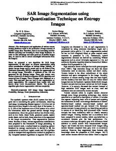
compared to per-pixel analyses is the consideration of spatial connection of individual pixels (Evans et al., 2009). It is possible to take into account the sizes, shapes and relevant positions of real-world image objects like terrain elements or landscape patterns across a stack of several environmental gradients (Blaschke and Strobl, 2001). There are different segmentation methods like histogrambased methods, edge detection, watershed segmentation or graph partitioning methods (Shapiro and Stockman, 2001). For our sampling optimization method we use a region growing algorithm as implemented in SAGA-GIS (Saga Development Team, 2010). This algorithm starts with a set of seed pixels which grows iteratively to homogenous objects in feature space until every pixel is assigned to a image object. A pixel merges with an adjacent pixel or a merged cluster of pixels, if its representativeness is the local maximum of all other neighboring free pixels. Detailed descriptions on the algorithm and on image segmentation in SAGA-GIS can be found in Böhner et al (2008) and Bechtel et al. (2008). 3. Case Study To demonstrate SegBS we compare our method with simple random sampling (SRS) and regular sampling (REG) in a study area around the northern foothills of the Alps in the south of Germany. For the delineation of terrain segments we used only terrain attributes as input feature space. As data input we used a 10m digital elevation model generated on airborne laser scanning data which guarantees high spatial accuracy. From this we derived 17 terrain attributes with the terrain analysis modules of SAGA-GIS. To find an optimal set of terrain attributes for delineating terrain segments we made a comprehensive comparison for all terrain attributes. In the end, we get proper results with slope, SAGA Wetness Index , and topographic position index. 3.1. Sampling As sampling locations for SegBS we simply use the centroides of the delineated image objects. Thereby the number of samplin points can be controled by the number of image objects. Since the region growing algorithm uses seed points as source for pixel merging the number of seed points is equal to the number of sampling points. As seeds we used systematic arranged points in order to cover the entire study area. To compare SegBS with SRS and REG we generate samples in eight different scales: 50, 75, 100, 125, 150, 200, 250 and 300 sampling points. 4. Results and discussion 4.1. Distribution of sampling points in geographic space As a measure of the well-balanced spatial distribution of sampling points we use the area of Voronoi polygons constructed around every sampling point. A Voronoi polygon associated with a given point of a point pattern X is the region of space that is closer to that point than to any other point of X (Okabe et al., 2000). Stevens and Olson (2004) propose a spatial efficiency ratio (ER) as a useful way to measure statistical efficiency of survey designs. They use the variance of the area of Voronoi polygons formed around every sampling point constructed with a specific sampling scheme compared to simple random sampling. If ER < 1.0, then the sampling design is more spatially efficient than SRS. Fig 1 shows ER-values for SegBS for eight different sampling intensities. Our method achieves a ratio between 0.23 and 0.55, which demonstrates that SegBS gives a spatially balanced sample.
2
Fig.1: Spatial efficiency ratio of SegBS. The ratio is calculated by the mean variance of Voronoi polygons around samples conducted with SegBS versus SRS.
Fig 2 shows boxplots of nearest neighbour distance for SegBS and SRS for eight sampling intensities. For every sampling intensity SegBS shows the lower interquartile range. The spacing between the lower quartile and the median reveals that there is always a sound spacing between the individual points in SegBS in contrast to SRS.
Fig.2: Distribution of nearest neighbor distance for SegBS and SRS for eight sampling intensities.
4.2. Distribution of sampling points in feature space Concerning feature space, a representative sample has to mimic the distribution of the underlying multivariate population. With “population” we mean the values of all raster cells in the entire study area, i.e. 172.800 raster cells. Fig. 3 shows density plots for slope and SAGA Wetness index (SWI) comparing SegBS, SRS, and REG in four sampling intensities: 50, 75, 150, and 250 sampling points. The dark grey background indicates the distribution of the population. The plots illustrate that SegBS shows the best representation of the population for slope and SWI, even with a low sampling intensity. The distribution at each sampling step sampled with the other methods slightly under-sampled areas, where the density plot reaches their maximum. The delineation of image objects based on multivariate feature space guarantees that SegBS represents the whole range of the statistical distribution. In areas with a high variance in feature space (here: areas with a heterogeneous relief) image objects become smaller and more sampling points are located so that we achieve an optimal representation of the original distribution (Fig 3). If the sampling intensity becomes higher the differences between the curves reduces.
3
Fig.3: Density plots for slope (column 1) and SAGA Wetness Index (column 2) for SegBS, SRS, and REG and for four sampling intensities (row one to four). The solid dark grey shadow indicates the underlying population (entire grid). The third column shows the single segments for every particular sampling intensity.
5. Conclusions We could show that by using image segmentation algorithms it is possible to get an optimized distribution of sampling points over an area of interest. In comparison to SRS and REG a sample constructed with SegBS fits the value distribution of the underlying population the best, especially
4
with low sampling intensities. At the same time sampling locations were distributed well-balanced over an area of interest. The segmentation algorithm used for this study has proven as useful, flexible, and reproducable tool for sampling optimization. Still it is easy to use and freely available in SAGA-GIS. One drawback about this region merging algorithm is that the main focal point is on the multivariate feature space rather than on the size and shape of image objects. If image objects becomes hugh and irregular the center of gravity may not be the best way to construct a sample. There are powerful and more flexible segmentation algorithms which overcomes this drawback (e.g. multi-resolution segmentation in the commercial software eCognition©). 6. References Bechtel, B., Ringeler, A. and Böhner, J. 2008. Segmentation for object extraction of trees using MATLAB and SAGA. In: J. Böhner, T. Blaschke and L. Montanarella (Editors), SAGA Seconds out. Hamburger Beiträge zur Physischen Geographie und Landschaftsökologie19. Hamburg, pp. 1-12. Blaschke, T. and Strobl, J. 2001. What’s wrong with pixels? Some recent developments interfacing remote sensing and GIS. GIS - Zeitschrift für Geoinformationssysteme, 6/2001: 12-17. Brus, D.J. and Heuvelink, G.B.M. 2007. Optimization of sample patterns for universal kriging of environmental variables. Geoderma, 138(1-2): 86-95. Burnett, C. and Blaschke, T. 2003. A multi-scale segmentation/object relationship modelling methodology for landscape analysis. Ecological Modelling, 168: 233-249. Drâgut, L. and Blaschke, T. 2006. Automated classification of landform elements using objectbased image analysis. Geomorpholohy, 81: 330-344. Drâgut, L., Schauppenlehner, T., Muhar, A., Strobl, J. and Blaschke, T. 2009. Optimization of scale and parametrization for terrain segmentation: An application to soil-landscape modeling. Computers & Geosciences, 35(9): 1875-1883. Evans, I.S., Hengl, T. and Gorsevski, P. 2009. Applications in Geomorphology. In: T. Hengl and H.I. Reuter (Editors), Geomorphometry. Concepts, Software, ApplicationsElsevier, Amsterdam, pp. 497-526. Gessler, P.E., Moore, I.D., McKenzie, N.J. and Ryan, P.J. 1995. Soil-landscape modelling and spatial prediction of soil attributes. International Journal of Geographical Information Science, 9(4): 421-432. Hengl, T., Rossiter, D.G. and Stein, A. 2003. Soil sampling strategies for spatial prediction by correlation with auxiliary maps. Australian Journal of Soil Research, 41(8): 1403-1422. Hengl, T. and Reuter, H.I. (Editors), 2009. Geomorphometry. Concepts, Software, Applications. Developments in Soil Science, 33. Elsevier, Amsterdam. MacMillan, R.A. and Shary, P.A. 2009. Landforms and Landform elements in Geomorphometry. In: T. Hengl and H.I. Reuter (Editors), Geomorphometry. Concepts, Software, Applications. Developments in Soil Science - Volume 33Elsevier, Amsterdam, pp. 227-254. Minasny, B. and McBratney, A. 2006. A conditioned Latin hypercube method for sampling in the presence of ancillary information. Computers & Geosciences, 32: 1378-1388. Minasny, B., McBratney, A.B. and Walvoort, D.J.J. 2007. The variance quadtree algorithm: Use for spatial sampling design. Computers & Geosciences, 33(3): 383-392. Möller, M., Volk, M., Friedrich, K. and Lymburner, L. 2008. Placing soil-genesis and transport processes into a landscape context: A multiscale terrain-analysis approach. Journal of Plant Nutrition and Soil Science-Zeitschrift für Pflanzenernährung und Bodenkunde, 171(3): 419430. Okabe, A., Boots, B., Sugihara, K. and Chiu, S.N. 2000. Spatial Tessellations: Concepts and Applications of Voronoi Diagrams. Wiley, West Sussex. Ryan, P.J., McKenzie, N.J., O'Connell, D., Loughhead, A.N., Leppert, P.M., Jacquier, D. and Ashton, L. 2000. Integrating forest soils information across scales: spatial prediction of soil properties under Australian forests. Forest Ecology and Management, 138(1-3): 139-157. 5
Saga Development Team, 2010, System for Automated Geoscientific Analyses (SAGA GIS). http://www.saga-gis.org/ (last verified 30.03.2010). Shapiro, L.G. and Stockman, G. 2001. Computer Vision. Prentice-Hall, New Jersey. Simbahan, G.C. and Dobermann, A. 2006. Sampling optimization based on secondary information and its utilization in soil carbon mapping. Geoderma, 133(3-4): 345-362. Vasát, R., Heuvelink, G.B.M. and Boruvka, L. 2010. Sampling design optimization for multivariate soil mapping. Geoderma, 155(3-4): 147-153.
6