Scalable Fine-grained Call Path Tracing Nathan R. Tallent
John Mellor-Crummey
Rice University
Rice University
[email protected] [email protected] Michael Franco Reed Landrum Laksono Adhianto Rice University
Stanford University
Rice University
[email protected]
[email protected]
[email protected]
ABSTRACT
1.
Applications must scale well to make efficient use of even medium-scale parallel systems. Because scaling problems are often difficult to diagnose, there is a critical need for scalable tools that guide scientists to the root causes of performance bottlenecks. Although tracing is a powerful performance-analysis technique, tools that employ it can quickly become bottlenecks themselves. Moreover, to obtain actionable performance feedback for modular parallel software systems, it is often necessary to collect and present fine-grained contextsensitive data — the very thing scalable tools avoid. While existing tracing tools can collect calling contexts, they do so only in a coarse-grained fashion; and no prior tool scalably presents both context- and time-sensitive data. This paper describes how to collect, analyze and present fine-grained call path traces for parallel programs. To scale our measurements, we use asynchronous sampling, whose granularity is controlled by a sampling frequency, and a compact representation. To present traces at multiple levels of abstraction and at arbitrary resolutions, we use sampling to render complementary slices of calling-context-sensitive trace data. Because our techniques are general, they can be used on applications that use different parallel programming models (MPI, OpenMP, PGAS). This work is implemented in HPCToolkit.
As hardware-thread counts increase in supercomputers, applications must scale to make effective use of computing resources. However, inefficiencies that do not even appear at smaller scales can become major bottlenecks at larger scales. Because scaling problems are often difficult to diagnose, there is a critical need for tools that guide scientists to the root causes of performance bottlenecks. Tracing has long been a method of choice for many performance tools [6,8,9,12,15,17,19,22,24,30,31,33,35,43,44]. Because performance traces show how a program’s behavior changes over time — or, more generally, with respect to a progress metric — tracing is an especially powerful technique for identifying critical scalability bottlenecks such as load imbalance, excessive synchronization, or inefficiencies that develop over time. For example, consider a trace that distinguishes between, on one hand, periods of useful work and, on the other, communication within the processes of a parallel execution. Presenting this trace as a Gantt chart, or process/time diagram, can easily show that load imbalance causes many processes to (unproductively) wait at a collective operation. In contrast, such a conclusion is often difficult to draw from a performance profile in which an execution’s time dimension has been collapsed. Although trace-based performance tools can yield powerful insight, they can quickly become a performance bottleneck themselves. With most tracing techniques, the size of each thread’s trace is proportional to the length of its execution. Consequently, for even medium-scale executions, extensive tracing can easily generate gigabytes or terabytes of data, causing significant perturbations in an execution when this data is flushed to a shared file system [5,8,14,15,23,25]. Moreover, massive trace databases create additional scaling challenges for analyzing and presenting the corresponding performance measurements. Because traces are so useful but so difficult to scale, much recent work has focused on ways to reduce the volume of trace data. Methods for reducing trace-data volume include lossless online compression [20, 30]; ‘lossy’ online compression [12]; online clustering for monitoring only a portion of an execution [13, 14, 25]; post-mortem clustering [5, 16, 24]; online filtering [16]; selective tracing (static filtering) [8, 15, 35]; and throttling [19, 35]. However, prior work on enhancing the scalability of tracing does not address three concerns that we believe are critical for achieving effective performance analysis that leads to actionable performance feedback.
Categories and Subject Descriptors C.4 [Performance of systems]: Measurement techniques, Performance attributes
General Terms Algorithms, Measurement, Performance
Keywords tracing, calling context, statistical sampling, performance tools, HPCToolkit
Permission to make digital or hard copies of all or part of this work for personal or classroom use is granted without fee provided that copies are not made or distributed for profit or commercial advantage and that copies bear this notice and the full citation on the first page. To copy otherwise, to republish, to post on servers or to redistribute to lists, requires prior specific permission and/or a fee. ICS’11, May 31–June 4, 2011, Tuscon, Arizona, USA. Copyright 2011 ACM 978-1-4503-0102-2/11/05 ...$10.00.
INTRODUCTION
First, prior work largely emphasizes flat trace data, i.e., traces that exclude additional execution context such as calling context. Because new applications employ modular design principles, it is often important to know not simply what an application is doing at a particular point, but also that point’s calling context. For instance, consider a case where one process in an execution causes all others to wait by performing additional work in a memory copy. The memory copy routine is likely called from many different contexts. To begin resolving the performance problem, it is necessary to know the calling contexts of the problematic memory copies. While some tracing tools have recently added support for collecting calling contexts, they do so in a relatively coarse-grained fashion, usually with respect to a limited set of function calls [12, 19, 21, 33]. Moreover, while these tools can show calling context for an individual trace record, no tool presents context- and time-sensitive data, across multiple threads, for arbitrary portions of an execution. In this paper, we show how to use sampling to present arbitrary and complementary slices of calling-context-sensitive trace data. Second, to reduce trace-data volume, prior tracing tools use, among other things, coarse-grained instrumentation to produce coarse-grained trace data. Examples of coarsegrained instrumentation include only monitoring high-level ‘effort loops’ [12] or MPI communication routines [44]. One problem with coarse-grained instrumentation is that, except where there is a pre-defined (coarse) monitoring interface (as with MPI [28]), manual effort or a training session is required to select instrumentation points. Another problem is that coarse-grained instrumentation may be insufficient to provide actionable insight into a program’s performance. For example, although a tool that only traces MPI communication can easily confirm the presence of load imbalance in SPMD (Single Program Multiple Data) programs, that tool may not be able to pinpoint the source of that imbalance in a complex modular application. Therefore, it is often desirable to scalably generate relatively fine-grained traces across all of an application’s procedures. However, using fine-grained instrumentation to generate a fine-grained trace has not been shown to be scalable. Indeed, instrumentation-based measurement faces an inelastic tension between accuracy and precision. For instance, instrumentation of small frequently executing procedures — which are common in modular applications — introduces overhead and generates as many trace records as procedure invocations. To avoid measurement overhead, we use asynchronous sampling to collect call path traces.1 Both coarsegrained instrumentation and sampling reduce the volume of trace data by selectively tracing. However, coarse-grained instrumentation often ignores that which is important for performance (such as small math or communication routines), whereas asynchronous sampling tends to ignore that which is least relevant to performance (such as routines that, over all instances, consume little execution time). Thus, because we use asynchronous sampling, our tracer monitors an execution through any procedure and at any point within a procedure, irrespective of a procedure’s execution frequency or length and irrespective of application and library boundaries. Because asynchronous sampling uses a controllable 1
Sampling can be synchronous or asynchronous with respect to program execution. Although we focus on the latter, there are important cases where the former is useful [40].
sampling frequency, our tracer has controllable measurement granularity and overhead. By combining sampling with a compact call path representation, our tracer can collect comparatively fine-grained call path traces (hundreds of samples/second) of large-scale executions and present them on a laptop. Third, while tools like ScalaTrace [30] exploit modelspecific knowledge to great effect, recent interest in hybrid models (e.g., OpenMP + MPI) and PGAS languages suggests that a more general approach can be valuable. Our sampling-based measurement approach is programmingmodel independent and can be used on standard operating systems (OS), as well as the microkernels used on the IBM Blue Gene/P and Cray XT supercomputers [39]. While we affirm the utility of exploiting model-specific properties, having the ability to place such insight in the context of an application’s OS-level execution is also valuable. In this paper, we describe measurement, analysis and presentation techniques for scalable fine-grained call path tracing. We make the following contributions: • We use asynchronous sampling to collect informative call path traces with modest cost in space and time. By combining sampling with a compact representation, we can generate detailed traces of large-scale executions with controllable granularity and overhead. Our method is general in that, instead of tracing certain aspects of a thread’s execution (such as MPI calls), we sample all activity that occurs in user mode. • We describe scalable techniques for analyzing a trace. In particular, we combine in parallel every thread-level call path trace so that all thread-level call paths are compactly represented in a data structure called a calling context tree. • We show how to use sampling to present (out-of-core) call path traces using two complementary views: (1) a process/time view that shows how different slices of an execution’s call path change over time; and (2) a call-path/time view that shows how a single process’s (or thread’s) call path changes over time. These techniques enable us to use a laptop to rapidly present trace files of arbitrary length for executions with an arbitrary number of threads. In particular, given a display window of height h and width w (in pixels), our presentation tool can render both views in time O(hw log t), where t is the number of trace records in the largest trace file. Our work is implemented within HPCToolkit [1, 32], an integrated suite of tools for measurement and analysis of program performance on computers ranging from multicore desktop systems to supercomputers. The rest of this paper is organized as follows. First, Section 2 presents a taxonomy of existing techniques for collecting and presenting traces of large-scale applications. Then, Sections 3, 4 and 5 respectively describe how we (a) collect call path traces of large-scale executions; (b) prepare those measurements for presentation using post-mortem analysis; and (c) present those measurements both in a scalable fashion and in a way that exposes an execution’s dynamic hierarchy. To demonstrate the utility of our approach, Section 6 presents several case studies. Finally, Section 7 summarizes our contributions and ongoing work.
2.
RELATED WORK
There has been much prior work on tracing. This section analyzes the most relevant work on call path tracing from the perspectives of measurement, presentation and scalability.
2.1
Collecting Call Path Traces
Because it is important to associate performance problems with source code, recently several tracing tools have added support for collecting the calling context of trace events [3, 12, 19, 21, 33]. However, instead of collecting detailed call path traces, these tools, with perhaps two exceptions, trace in a relatively coarse-grained manner. The reason is that most of these tools measure using forms of static or dynamic instrumentation. Because instrumentation is inherently synchronous with respect to a program’s execution, fine-grained instrumentation — such as instrumenting every primitive in a math library — causes both high measurement overhead and an unmanageable volume of trace data. Consequently, to scale well, instrumentation-based tools rely on coarse-grained instrumentation, which results in coarsegrained traces. For instance, a common tracing technique is to trace MPI calls and collect the calling context of either (a) each MPI call [19,21,33] or (b) the computation between certain MPI calls [12]. Moreover, some of these tools encourage truncated calling contexts. With the CEPBA Tools, one can specify a ‘routine of interest’ to stop unwinds [21]; with VampirTrace, one specifies a call stack depth [41]. Two existing tools — the exceptions mentioned above — can collect fine-grained traces. The CEPBA Tools combine coarse-grained instrumentation and asynchronous sampling to generate flat fine-grained traces supplemented with coarse-grained calling contexts [21, 34]. Apple Shark uses asynchronous sampling and stack unwinding to collect finegrained call path traces [3]. Both of these tools collect finegrained data because they employ asynchronous sampling. Apple Shark [3] is perhaps the closest to our work, at least with respect to measurement. However, there are three critical differences. First, as a single-node system-level tracer, Shark is designed to collect data, not at the application level, but at the level of a hardware thread. As a result, it cannot per se trace a parallel application with multiple processes. Second, to our knowledge, Shark does not use a compact structure (like a calling context tree [2]) to store call paths. Third, Shark is not always able to unwind a thread’s call stack. It turns out that unwinding a call stack from an arbitrary asynchronous sample is quite challenging when executing optimized application binaries. Because we base our work on dynamic binary analysis for unwinding call stacks [38], HPCToolkit can accurately collect full call path traces, even when using asynchronous sampling of optimized code. Besides affecting trace granularity, a tool’s measurement technique also affects the class of applications the tool supports. Because MPI is dominant in large-scale computing, a number of tools primarily monitor MPI communication [12, 30, 31, 34, 44]; some also include support for certain OpenMP events. However, both technology pressure and programming-productivity concerns have generated much interest in alternative models such as PGAS languages. Our approach, which measures arbitrary computation within all threads of an execution, easily maps to all of these models. Additionally, an approach that monitors at the system level can take advantage of a specific model’s semantics to provide
trace information both at the run-time level (for run-time tuning) and at the application level [37].
2.2
Presenting Call Path Traces
Although a few tools collect coarse call path traces, no tool presents context-sensitive data for arbitrary portions of the process and time dimensions. For instance, one especially important feature for supporting top-down contextual analysis is the ability to arbitrarily zoom. To do this, a tool must be able to (a) appropriately summarize a large trace within a relatively small amount of display real estate; (b) render high-resolution views of interesting portions of the execution; and (c) expose context. While presentation tools such as Paraver [22], Vampir [19] and Libra [12] display flat trace data across arbitrary portions of the process and time dimensions, they do not analogously present call path data. Instead, current presentation techniques for call path traces are limited to displaying different forms of one thread’s call path. For instance, Apple Shark [3] presents call path depth with respect to one hardware thread. Thus, it shows stylized call paths (i.e., the depth component) for all application threads that execute on a particular hardware thread. While this is interesting from a system perspective, it is not helpful from the perspective of a parallel application. Open|SpeedShop displays call paths of individual trace events [33]. While this is very useful for finding where in source code a trace event originates, it does not provide a high-level view of the dynamic structure of an execution. Vampir can display a ‘Process Timeline’ that shows how caller-callee relationships unfold over time for a single process [19]. While the ability to see call paths unfolding over time is helpful, only focusing on one process can be limiting.
2.3
Scaling Trace Collection and Presentation
Because traces are so useful but so difficult to scale, much recent work has focused on ways to reduce the volume of trace measurement data. Broadly speaking, there are two basic techniques for reducing the amount of trace information: coarse measurement granularity and data compression. Since as discussed above (Subsection 2.1), nearly all tools measure in a coarse-grained fashion, here we focus primarily on compression techniques, which can be lossless or ‘lossy.’ As an example of lossless compression, ScalaTrace relies on program analysis to compress traces by compactly representing certain commonly occurring trace patterns [30]. For applications that have analyzable patterns, ScalaTrace’s approach is extremely effective for generating compressed communication traces. VampirTrace uses a data structure called a Compressed Complete Call Graph to represent commonality among several trace records [20]. Similarly, we use a calling context tree [2] to compactly represent trace samples. There are several forms of ‘lossy’ compression. Gamblin et al. have explored techniques for dynamically reducing the volume of trace information such as (a) ‘lossy’ online compression [12]; and (b) online clustering for monitoring only a subset of the processes in an execution [13, 14]. They report impressively low overheads, but they also, in part, use selective instrumentation that results in coarse measurements. A popular form of ‘lossy’ compression is clustering. Lee et al. reduce trace file size by using k-Means clustering to select representative data [23, 24]. However, because their datareduction technique is post-mortem rather than online, it
assumes all trace data is stored in memory. This is feasible only with coarse-grained tracing. The CEPBA Tools can use both offline and online clustering techniques for reducing data [5,16,22,25]. To make trace analysis and presentation more manageable, Casas et al. developed a post-mortem technique to compress a trace by identifying and retaining representative trace structure [5]. Going one step further, to reduce the amount of generated trace data, Gonzalez et al. [16] and Llort et al. [25] developed online clustering algorithms to retain only a representative portion of the trace. It is not clear how well these techniques would work for fine-grained call path tracing. Yet another way to ‘lossily’ compress trace data is to filter it. As already mentioned, to manage overhead, all instrumentation-based tools statically filter data by selectively instrumenting. Scalasca and TAU support feedbackdirected selective tracing, which uses the results of a prior performance profile to avoid instrumenting frequently executing procedures [15, 35]. Others tools support forms of manual selective tracing [8]. Since feedback-directed trace reduction requires an additional execution, it is likely impractical in some situations; and manual instrumentation is usually undesirable. In contrast to static filtering, it is also possible to dynamically filter trace information. For example, the CEPBA Tools dynamically filter trace records by discarding periods of computation that consume less than a certain time threshold [16]. While dynamic filtering can effectively reduce trace data volume, it must be applied carefully to avoid systematic error by discarding frequent computation periods just under the filtering threshold. As another example of dynamic filtering, TAU and VAMPIR can optionally throttle a procedure by disabling its instrumentation after that procedure has been executed a certain number of times [19, 35]. In contrast to all of these techniques, by using asynchronous sampling, we have taken a fundamentally different approach to scale the process of collecting a call path trace. Although, we do use a form of lossless compression (a calling context tree), that compression would be ineffective without sampling. With a reasonable sampling period and the absence of a correlation between the execution and sampling period, asynchronous sampling can collect representative and fine-grained call path traces for little overhead. Sampling naturally focuses attention on important execution contexts without relying on possibly premature local filtering tests. Additionally, because asynchronous sampling provides controllable measurement granularity, it naturally scales to very large-scale and long-running executions. Sampling can also be employed to present call path traces at multiple levels of abstraction and at arbitrary resolutions. Here the basic problem is that a display window typically has many fewer pixels than available trace records. Given one pixel and the trace data that could map to it, sophisticated presentation tools like Paraver attempt to select the most interesting datum to define that pixel’s color [22]. However, such techniques require examination of all trace data to render one display. Because this is impractical for fine-grained traces of large-scale executions, we use various forms of sampling to rapidly render complementary slices of calling-context-sensitive data. In particular, by sampling trace data for presentation, we can accurately render views by consulting only a fraction of the available data.
(a) Call path sample return address
(b) Calling Context Tree (CCT) “main”
return address return address instruction pointer
sample point
Figure 1: (a) The call path for a sample point; (b) several call path samples form a calling context tree.
Other work on scalably presenting traces at multiple levels of resolution has focused on flat traces; and none, to our knowledge, has used sampling. To scale in the time dimension, Jumpshot’s SLOG2 format organizes trace events with a binary tree to quickly select trace events for rendering [7]. To scale in the time and process dimensions, Gamblin et al. use multi-level wavelet compression [12]. Lee et al. precompute certain summary views [23].
2.4
Summary
By using sampling both for measurement and presentation, we can collect and present fine-grained large-scale traces for applications written in several programming models. In prior work [1], we presented a terse overview of an early prototype of our tool. This paper, besides describing the key ideas behind our work, additionally presents new techniques for (a) scalable post-mortem trace analyses and (b) scalable presentation, including a combined process/time and call-path/time display.
3.
COLLECTING CALL PATH TRACES
To collect call path traces with controllable granularity and measurement overhead, we use asynchronous sampling. Sampling-based measurement uses a recurring event trigger, with a configurable period, to raise signals within the program being monitored. When an event trigger occurs, raising a signal, we collect the calling context of that sample — the set of procedure frames active on the call stack — by unwinding the call stack. Because unwinding call stacks from an arbitrary execution point can be quite challenging, we base our work on HPCToolkit’s call path profiler [38, 39]. To make a call path tracer scalable, we need a way to compactly represent a series of timestamped call paths. Rather than storing a call path independently for each sample event, we represent all of the call paths for all samples (in a thread) as a calling context tree (CCT) [2], which is shown in Figure 1. A CCT is a weighted tree whose root is the program entry point and whose leaves represent sample points. Given a sample point (leaf), the path from the tree’s root to the leaf’s parent represents a sample’s calling context. Although not strictly necessary for a trace, leaves of the tree can be weighted with metric values such as sample counts that represent program performance in context (a call path profile). The critical thing for tracing is that with a CCT, the calling context for a sample may be completely represented by a leaf node. Thus, to form a trace, we simply generate a sequence
of tuples (or trace records), each consisting of a 4-byte CCT node id and an 8-byte timestamp (in microseconds). With this approach, it is possible to obtain a very detailed call path trace for very modest costs. Assuming both a reasonable sampling rate — we frequently use rates of hundreds to thousands of samples per second — and a time-related sampling trigger, we can make several observations. First, assuming no correlation between an application’s behavior and the sampling frequency, our traces should be quite representative. Second, in contrast to instrumentation-based methods where trace-record generation is related to a procedure’s execution frequency, our rate of trace-record generation is constant. For instance, using a sampling rate of 1024 samples per second, our tracer generates 12 KB/s per thread of trace records (which are written to disk using buffered I/O); it writes the corresponding calling context tree at the end of the execution. Such modest I/O bandwidth demands are easily met. For instance, consider tracing an execution using all cores (≈ 160, 000) of Argonne National Laboratory’s Blue Gene/P system, Intrepid. At 12 KB/s per core, our bandwidth needs would be 0.0028% of Intrepid’s disk bandwidth per core [42]. Third, the total volume of trace records is proportional to the product of the sampling frequency and the length of an execution. (The size of the CCT is proportional to the number of distinct calling contexts exposed by sampling.) This means that an analyst has significant control over the total amount of trace data generated for an execution. Fourth, because our tracer uses a technique to memoize call stack unwinds [11], the overhead of collecting call paths is proportional only to the call stack’s new procedure frames with respect to the prior sample. Of course, there are conditions under which sampling will not produce accurate data. If the sampling frequency is too high, measurement overhead can significantly perturb the application. Another more subtle problem is when the sampling frequency is below the natural frequency of the data. Although typically not a problem with profiling (which conceptually generates a histogram of contexts and therefore aggregates small contexts), under-sampling is a real concern for tracing since traces approximate instantaneous behavior over time. It turns out, however, that under-sampling is not a significant problem for our tracer because of two reasons. First, most of the interesting time-based patterns occur not at call-path leaves, but within call-path interiors, which have lower natural frequencies. This might seem to defeat the purpose of fine-grained sampling. However, it is helpful to observe that our tracer’s call paths expose all implementation layers of math and communication libraries. Thus, frequently it is the case that moving out a few levels from a singly-sampled leaf brings an analyst to a multiplysampled interior frame that is still in a library external to the application’s source code (cf. Section 6). Second, for typical applications, selecting reasonable sampling frequencies that highlight an application’s representative behavior is not difficult. In particular, we typically use frequencies in the hundreds and thousands of samples per second which yields several samples for instances of interior procedure frames. Of course, any one sample may correspond to noise and one cannot assume that any particular call path leaf executed for the duration of the virtual time represented by a pixel. But our experience is that trace patterns at interior call-path frames are representative of an application’s execution.
4.
ANALYZING CALL PATH TRACES
To present the large-scale trace measurements of Section 3, it is helpful to perform several post-mortem analyses. These analyses are designed to (a) compress the measurement data; (b) enable its rapid presentation; and (c) associate measurements with static source code structure. Our work extends HPCToolkit’s analysis tool [36, 38]. This section focuses on the most important of these analyses. Recall that a thread’s trace is represented as a sequence of trace records and a calling context tree (CCT). Although generating distinct CCTs avoids communication and synchronization during measurement, it generates more total data than is necessary. For instance, in SPMD scientific applications, many thread-level CCTs have common structure. To significantly compress the total trace data, we create a canonical CCT that represents all thread-level CCTs. In many situations, we expect the canonical CCT to be no more than a small constant factor larger than a typical threadlevel CCT. To form the canonical CCT, we union each thread-level CCT so that a call path appears in the canonical CCT if and only if it appears in some thread-level CCT. We do this in parallel using a (tree-based) CCT reduction. An important detail is that the CCT reduction must ensure trace-file consistency, because each trace file must now refer to call paths in the canonical CCT instead of that thread’s CCT. Consider the case of merging a path from a thread-level CCT into the canonical CCT. Either the path (1) already or (2) does not yet exist in the canonical CCT. For case (1), let the path in the CCT be x and the other path be y. Even though x and y have exactly the same structure (call chain), in general, they have different path identifiers (IDs). When these paths are merged to form one path, we only want to retain one ID. Assuming that we keep x’s ID, it is then necessary to update trace records that refer to y. For case (2), when adding a path to the canonical CCT, it is necessary to ensure that that a path’s ID does not conflict with any other ID currently in the canonical CCT. If there is a conflict, we generate a new ID and update the corresponding trace records. For efficiency, we batch all updates to a particular trace file.
5.
PRESENTING CALL PATH TRACES
The result of Section 4’s analysis is a trace database. To interactively present these trace measurements, an analyst uses HPCToolkit’s hpctraceviewer presentation tool, which can present a large-scale trace without concern for the scale of parallelism it represents. To make this scalability possible, and to show call path hierarchy, we designed several novel presentation techniques for hpctraceviewer. This section discusses those techniques.
5.1
Presenting Call Path Hierarchy
To analyze performance effectively, it is necessary to rapidly identify inefficient execution within vast quantities of performance data. This means that, among other things, it is necessary to present data at several levels of detail, beginning with high-level data from which one can descend to lower-level data to understand program inefficiencies in more detail. Additionally, to understand multi-dimensional data, it is often necessary to view it from several different angles. Consequently, we have designed hpctraceviewer’s interface to facilitate rapid top-down performance analysis
Figure 2: An 8184-core execution of PFLOTRAN on a Cray XT5. The inset exposes call path hierarchy by showing the selected region (top left) at different call path depths. by displaying trace measurements in different views and at arbitrary levels of detail. In discussing the interface, we first describe hpctraceviewer’s views and then how those views can be manipulated; we defer case studies to Section 6. Figure 2 shows hpctraceviewer’s main display. It represents an execution of PFLOTRAN (see Section 6.1) that took 982 seconds on 8184 cores of a Cray XT5. The figure is divided into three panes. The two stacked horizontal panes on the left consume most of the figure and display the Trace View and Depth View. The third slender vertical pane on the right shows the Call Path View and, on the very bottom, the Mini Map. These four coordinated views are designed to show complementary aspects of the call path trace data: • Trace View (left, top): This is hpctraceviewer’s primary view. This view, which is similar to a conventional process/time (or space/time) view, shows time on the horizontal axis and process (or thread) rank on the vertical axis; time moves from left to right. Compared to typical process/time views, there is one key difference. To show call path hierarchy, the view is actually a user-controllable slice of the process/time/callpath space. Given a call path depth, the view shows the color of the currently active procedure at a given time and process rank. (If the requested depth is deeper than a particular call path, then hpctraceviewer simply displays the deepest procedure frame and, space permitting, overlays an annotation indicating the fact that this frame represents a shallower
depth.) Figure 2 shows that at depth 3, PFLOTRAN’s execution alternates between two phases (purple and black). The figure contains an inset that shows the boxed area (top left) in greater detail at call path depths of 3, 6, 7 and 14. At depth 6, it is apparent that the two phases use the same solver (tan), though depths 7 and 14 show that they do so in different ways. hpctraceviewer assigns colors to procedures based on (static) source code procedures. Although the color assignment is currently random, it is consistent across the different views. Thus, the same color within the Trace and Depth Views refers to the same procedure. The Trace View has a white crosshair that represents a selected point in time and process space. For this selected point, the Call Path View shows the corresponding call path. The Depth View shows the selected process. • Depth View (left, bottom): This is a call-path/time view for the process rank selected by the Trace View’s crosshair. Given a process rank, the view shows for each virtual time along the horizontal axis a stylized call path along the vertical axis, where ‘main’ is at the top and leaves (samples) are at the bottom. In other words, this view shows for the whole time range, in qualitative fashion, what the Call Path View shows for a selected point. The horizontal time axis is exactly aligned with the Trace View’s time axis; and the
colors are consistent across both views. This view has its own crosshair that corresponds to the currently selected time and call path depth. • Call Path View (right, top): This view shows two things: (1) the current call path depth that defines the hierarchical slice shown in the Trace View; and (2) the actual call path for the point selected by the Trace View’s crosshair. (To easily coordinate the call path depth value with the call path, the Call Path View currently suppresses details such as loop structure and call sites; we may use indentation or other techniques to display this in the future.) • Mini Map (right, bottom): The Mini Map shows, relative to the process/time dimensions, the portion of the execution shown by the Trace View. The Mini Map enables one to zoom and to move from one close-up to another quickly. To further support top-down analysis, hpctraceviewer includes several controls for changing a view’s aspect and navigating through various levels of data: • The Trace View can be zoomed arbitrarily in both of its process and time dimensions. To zoom in both dimensions at once, one may (a) select a sub-region of the current view; or (b) select an arbitrary region of the Mini Map. To zoom in only one of the above dimensions, one may use the appropriate control buttons at the top of the Trace View. At any time, one may return to the entire execution’s view by using the ‘Home’ button. • To expose call path hierarchy, the call-path-depth slice shown in the Trace View can be changed by using the Call Path View’s depth text box or by selecting a procedure frame within the Call Path View. • To pan the Trace and Depth Views horizontally or vertically, one may (a) use buttons at the top of the Trace View pane; or (b) adjust the Mini Map’s current focus. Even though hpctraceviewer supports panning, it is worth noting that zooming is much more important because it permits viewing the execution at different levels of abstraction. In contrast, a tool that requires scrolling through vast quantities of data is difficult to use because, at any one time, the tool can only present a fraction of the execution.
5.2
Using Sampling for Scalable Presentation
To implement the arbitrary zooming that is required to support top-down analysis, it is clearly not feasible either (a) to examine all trace data repeatedly and exhaustively or (b) to precompute all possible (or likely) views. One possible solution for displaying data at multiple resolutions is to precompute select summary views [23]. We prefer a method that dynamically and rapidly renders views at arbitrary resolutions. Consider a large-scale execution that has tens of thousands of processor ranks and that runs for thousands of seconds, where time granularity is a microsecond. A trace of this scale dwarfs any typical computer display; today, a high-end 30-inch display we use has a width and height of 2560 × 1600 pixels. Thus, the basic problem that a trace
presentation tool faces is the following: Given a display window of a certain size, how should that window be rendered in time that is proportional not to the total amount of trace data, but to the window size? Alternatively, we can ask: given that one pixel maps to many trace records from many process ranks, how should we color that pixel without consulting all of the associated trace records? In this connection, it is helpful to briefly consider the presentation technique of conveying the maximum possible information about an application’s behavior [22]; cf. [23]. For example, to color one pixel, one could use either the minimum or maximum of the metric values associated with the trace records mapped to the pixel. While this can be a very effective way of rendering performance, it limits the scalability of a presentation tool because it requires examining every trace record mapped to the pixel. In contrast, to render the views described in Section 5.1 without concern for the scale of parallelism they represent, we use various forms of sampling. For example, consider the Trace View, which displays procedures at a given call path depth along the process and time axes. To render this view in a display window of height h and width w, hpctraceviewer does two things. First, it systematically samples the execution’s process ranks to select h ranks and their corresponding trace files. (For the trivial case where the number of process ranks is less than or equal to h, all ranks are represented.) Second, hpctraceviewer uses a form of systematic sampling to select the call path frames displayed along the process rank’s time lines. It subdivides the time interval represented by the entire execution into a series of consecutive and equal intervals using w virtual timestamps. Then, for each virtual timestamp, it binary searches the corresponding trace file — our trace file format is effectively a vector of trace records — to locate the record with the closest actual timestamp; this record’s call path is used to define the pixel’s color. We can make several observations about this scheme. Because we consult at most h trace files and perform at most w binary searches in each trace file, the time it takes to render the Trace View is O(hw log t), where t is the number of trace records in the largest trace file. In practice, the log t factor is often negligible because we use linear extrapolation to predict the locations of the w trace records. Next, as with the Trace View, the Depth View can also be rendered in time O(hw log t) by considering at most h frames of each call path. For some zooms and scrolling it is possible to reuse previously computed information to further reduce rendering costs. Finally, by generating virtual timestamps and using binary search, we effectively overlay a binary tree on the trace data, which is the basic idea behind Jumpshot’s SLOG2 trace format [7]. One problem with sampling-based methods is that while they tend to show representative behavior, they might miss interesting extreme behavior. While this will always be a problem with statistical methods, two things attenuate these concerns. First, we (scalably) precompute special constantsized values (instead of views) for hpctraceviewer. For example, we compute, for all trace files, the minimum beginning timestamp and the maximum ending timestamp, which takes work proportional to the number of processor ranks. Though a minor contribution, these timestamps enable hpctraceviewer’s Trace View to expose, e.g., extreme variation in an application’s launch or teardown. Second, and more
to the point, assuming an appropriately sized and uncorrelated sample, we expect sampling-based methods to expose anomalies that generally affect an execution. In other words, although using sampling-based methods for rendering a high-level view can easily miss a specific anomaly, those same methods will expose the anomaly’s general effects. If the anomaly does not interfere with the application’s execution, then a high-level view will show no effects. But if process synchronization transfers the anomaly’s effects to other process ranks, we expect sampling-based methods to expose that fact. It is worth noting that Figure 2 actually exposes an interesting anomaly. The thin horizontal white lines in the Trace View represent a few processes for which sampling simply stopped, most likely (we suspect) because of a kernel bug.2 One possible avenue of future work is for an analyst to identify a region and request a more exhaustive root-cause analysis. We are currently working on a Summary View that shows for each virtual timestamp a stacked histogram that qualitatively represents the number of process ranks executing a given procedure at a given call path depth. This view would be similar to Vampir’s ‘Summary Timeline’ [19]. However, in contrast to Vampir, which, to our knowledge, computes its view based on examining the activity of each thread at each time interval, we will use a sampling-based method to scalably render the view. To render this view for a window of height h and width w, we will first generate a series of w virtual timestamps as with the Trace View. Then, to create a stacked histogram for a given virtual timestamp, we will take a random sample of the process ranks and from there determine the set of currently executing procedures. The time complexity of rendering this view is the same as for the Trace View. Unlike many other tools, hpctraceviewer does not render inter-process communication arcs. We are uncertain how to do this effectively and scalably. Instead, we are exploring ways of using a special color, say red, to indicate, at all levels of a call path, when a sample corresponds to communication.
6.
CASE STUDIES
To demonstrate the ability of our tracing techniques to yield insight into the performance of parallel executions, we apply them to study the performance of the PFLOTRAN ground water flow simulation application [26, 29]; the FLASH [10] astrophysical thermonuclear flash code; and two HPC Challenge benchmark codes [18] written in Coarray Fortran 2.0, one implementing a parallel one-dimensional Fast Fourier Transform (FFT), and the second implementing High Performance Linpack, (HPL) which solves a dense linear system on distributed memory computers. We describe our experiences with each of these applications in turn.
6.1
PFLOTRAN
PFLOTRAN models multi-phase, multi-component subsurface flow and reactive transport on massively parallel computers [26, 29]. It uses the PETSc [4] library’s NewtonKrylov solver framework. We collected call path traces of PFLOTRAN running on 8184 cores of a Cray XT5 system known as JaguarPF, which 2
This process could not have stopped because the execution’s many successful collective-communication operations would not have completed.
is installed at Oak Ridge National Laboratory. The input for the PFLOTRAN run was a steady-state groundwater flow problem. To collect traces, we configured HPCToolkit’s hpcrun to sample wallclock time at a frequency of 200 samples/second. Tracing dilated the application’s execution by 5% and the total job (including the time for hpcrun to flush measurements to disk) by 10%. hpcrun generated 13 GB of data (1.6 MB/process); a parallel version of HPCToolkit’s hpcprof analyzed the measurements in 13.5 minutes using 48 cores and generated a 7.5 GB trace database. Figure 2 shows hpctraceviewer displaying a high level overview of a complete call path trace of a 16 minute execution of PFLOTRAN on 8184 cores. Recall from Section 5.1 that (a) the Trace View (top) shows a process/time view; (b) the Depth View shows a time-line view of the call path for the selected process; and (c) the Call Path View (right) shows a call path for the selected time and process. A process’s activity over time unfolds from left to right. Unlike other trace visualizers, hpctraceviewer’s visualizations are hierarchical. Since each sample in each process’s timeline represents a call path, we can view the process timelines at different call path depths to show more or less detailed views of the execution. The figure shows the execution at a call path depth of 3. Each distinct color on the timelines represents a different procedure executing at this depth. The figure clearly shows the alternation between PFLOTRAN’s flow (purple) and transport (black) phases. The beginning of the execution shows different behavior as the application reads its input using the HDF5 library. The figure contains an inset that shows the boxed area (top left) in greater detail at call path depths of 3, 6, 7 and 14. At depth 6, it is apparent that the flow and transport phases use the same solver (tan), though depths 7 and 14 show that they do so in different ways. The point selected by the crosshair shows the flow phase performing an MPI_Allreduce on behalf of a vector dot product (VecDotNorm2) deep within the PETSc library. The call path also descends into Cray’s MPI implementation. Given that the routine MPIDI_CRAY_Progress_wait (eighth from the bottom) is associated with exposed waiting, we can infer that the flow phase is currently busy-waiting for collective communication to complete.
6.2
FLASH
Next we consider FLASH [10], a code for modeling astrophysical thermonuclear flashes. Figure 3 shows hpctraceviewer displaying an 8184-core JaguarPF-execution of FLASH. We used an input for simulating a white dwarf detonation. It is immediately apparent that the first 60% of execution is quite different than the regular patterns that appear thereafter. The Trace View’s crosshair marks the approximate transition point. At this point, the Call Path View makes clear that the execution is still in its initialization phase (cf. driver_initflash at depth 2). Note the large light purple region on the left that consumes about one-third of the execution. A small amount of additional inspection reveals that this corresponds to a routine which simply calls MPI_Init. Note also that there are a few white lines that span the length of this light purple segment. These lines correspond to straggler MPI ranks which took about 190 seconds to launch — no samples can be collected until a process starts — and arrive at MPI_Init, which is acting like a collective operation. In other words, recalling the discussion in Section 5.2, a few anomalous processors had
Figure 3: An 8184-core execution of FLASH on a Cray XT5. enormous effects on the execution and sampling-based presentation techniques immediately exposed them.
6.3
High Performance Linpack (HPL)
Figure 4 shows our tool displaying a 5000 second execution of an implementation of High Performance Linpack written in Rice University’s Coarray Fortran 2.0 [27] running on 256 cores of a Cray XT4. The blue triangular sections show serialization present in initialization and finalization code. The center section of the figure shows the heart of the LU decomposition. The irregular moire patterns arise because of the use of asynchronous broadcast communication, which allows the execution to proceed without tight synchronization between the processes.
6.4
Fast Fourier Transform (FFT)
Figure 5 shows our tool displaying a 76 second execution of an implementation of a one-dimensional implementation of Fast Fourier Transform (FFT) written in Rice University’s Coarray Fortran 2.0 [27] running on 256 cores. The figure displayed here shows the first execution we traced to begin to understand (a) the overall performance of the code, (b) the impact of different regions of the code on its execution time, and (c) the transient behavior of the code. We were surprised by what we found in the trace. The FFT computation has several distinct phases: an all-to-all permutation, a local computation phase that is proportional to N log N (where N is the size of the local data), and finally a global computation phase that requires N log P time and log P rounds of pairwise asynchronous communication. In the Trace View, the green samples represent execution of calls to barrier synchronization. The application has only two barriers: one at the beginning of the global communication phase and one end. While the first (leftmost) barrier is short — indicated by the narrow green band, the barrier at the end consumes 30% of the total execution time! This
diagram revealed that even though the global communication phase should be evenly balanced across the processors, in practice some processors were finishing much later than others. Processors that finish in a timely fashion wait at the barrier until the stragglers arrive. The inset figure shows detail from the interior of the execution. The blue areas show processors waiting for asynchronous get operations to complete. We have concluded that this is an effect rather than a cause of the imbalance. The cursor selection in the inset shows an unexpected stall inside our asynchronous progress engine. The stall occurred within a call to the GASNet communication library that checks for the completion of a non-blocking get. In our use of GASNet, we had not anticipated that calls to non-blocking primitives would ever block. Clearly, our expectations were wrong. Based on the feedback from hpctraceviewer, we implemented an alternate version of FFT that used all-to-all communication rather than the problematic asynchronous pairwise communication. The changes resulted in a 50% speedup when executed on 4096 cores of a Cray XT4 known as Franklin.
6.5
Summary
We have demonstrated our tools on applications with several different behaviors and over two very different programming models (MPI and Coarry Fortran 2.0). Our samplingbased trace presentation quickly exposed several things: extremely late launching for a few processes (FLASH), serialization during HPL’s initialization and finalization; and delays caused by asynchronous communication in what should have been a balanced phase (FFT). We show call paths that begin at ‘main,’ descend into libraries (e.g., PETSc), and continue into libraries used by those libraries (e.g., MPI). By exposing this detail, an informed analyst can form very precise hypotheses about what is happening, such as our
Figure 4: A 256-core execution of a Coarray Fortran 2.0 implementation of High Performance Linpack on a Cray XT4. hypothesis that FFT is using GASNet in such a way as to exhaust its asynchronous get resource tickets. We believe this provides strong evidence that our sampling-based trace presentation is not only scalable, but is also highly effective in exposing performance problems and even some anomalies.
7.
CONCLUSIONS
The fundamental theme of this paper is how to use various forms of sampling to collect and present fine-grained call path traces. To collect call path traces of large-scale executions with controllable measurement granularity and overhead, we use asynchronous sampling. By combining sampling with a compact representation of call path trace data, we generate trace data at a very moderate, constant and controllable rate. (Additionally, by using a technique to memoize call stack unwinds, it is only necessary to unwind procedure frames that are new with respect to the prior sample.) To rapidly present trace data at multiple levels of abstraction and in complementary views, hpctraceviewer, again, uses various sampling techniques. We showed that sampling-based presentation is not only rapid, but can also be effective. Given all this, we would argue that HPCToolkit’s call path tracer manages measurement overhead and data size better than a typical flat tracer — while providing more detail. Our sampling-based measurement approach naturally applies to many programming models because it measures all aspects of a thread’s user-level execution. While there are cases, such as over-threading, where measuring systemlevel threads does not well match the application-level programming model, our approach does not preclude exploiting model-specific knowledge as well. There are a number of directions that we are actively exploring. First, we want to use our sampling-based call path trace information to identify root causes of performance bottlenecks; related work would be pattern analyzers for instrumentation based-tracing. A starting point is to use a special color, say red, to indicate, at all levels of a call path, when a sample corresponds to communication. Second, with an eye
toward exascale computers, we are exploring measurement techniques that involve sampling at multiple levels, such as randomly sampling processes that are then monitored for a period using asynchronous sampling. Third, we want to add several modest but very useful features. As one example, we would like to expose structure within a procedure frame (including sample points) and link it to source code, just as we do with HPCToolkit’s hpcviewer tool for presenting call path profiles. As another example, we plan to track a sampled procedure’s return to distinguish, in the Depth View, between several samples (a) within the same procedure instance and (b) spread over different procedure instances. Finally, we are considering techniques for addressing clock skew, a classic problem with tracing.
Acknowledgments Guohua Jin wrote the Coarry Fortran (CAF) 2.0 version of HPL; Bill Scherer wrote the CAF 2.0 version of FFT. Development of HPCToolkit is supported by the Department of Energy’s Office of Science under cooperative agreements DE-FC02-07ER25800 and DE-FC0206ER25762. This research used resources of (a) the National Center for Computational Sciences at Oak Ridge National Laboratory, which is supported by the Office of Science of the U.S. Department of Energy under contract DE-AC0500OR22725; (b) the National Energy Research Scientific Computing Center, which is supported by the Office of Science of the U.S. Department of Energy under contract DEAC02-05CH11231; and (c) the Argonne Leadership Computing Facility at Argonne National Laboratory, which is supported by the Office of Science of the U.S. Department of Energy under contract DE-AC02-06CH11357.
8.
REFERENCES
[1] L. Adhianto, S. Banerjee, M. Fagan, M. Krentel, G. Marin, J. Mellor-Crummey, and N. R. Tallent. HPCToolkit: Tools for performance analysis of optimized parallel programs. Concurrency and
Figure 5: A 256-core execution of a Coarray Fortran 2.0 FFT benchmark on a Cray XT4. The inset shows detail around the main crosshair.
[2]
[3] [4]
[5]
[6]
[7]
[8]
[9]
Computation: Practice and Experience, 22(6):685–701, 2010. G. Ammons, T. Ball, and J. R. Larus. Exploiting hardware performance counters with flow and context sensitive profiling. In Proc. of the 1997 ACM SIGPLAN Conf. on Programming Language Design and Implementation, pages 85–96, New York, NY, USA, 1997. ACM. Apple Computer. Shark User Guide, April 2008. S. Balay, K. Buschelman, V. Eijkhout, W. D. Gropp, D. Kaushik, M. G. Knepley, L. C. McInnes, B. F. Smith, and H. Zhang. PETSc users manual. Technical Report ANL-95/11 - Revision 3.0.0, Argonne National Laboratory, 2008. M. Casas, R. Badia, and J. Labarta. Automatic structure extraction from MPI applications tracefiles. In A.-M. Kermarrec, L. Boug´e, and T. Priol, editors, Proc. of the 13th Intl. Euro-Par Conference, volume 4641 of Lecture Notes in Computer Science, pages 3–12. Springer, 2007. J. Caubet, J. Gimenez, J. Labarta, L. De Rose, and J. S. Vetter. A dynamic tracing mechanism for performance analysis of OpenMP applications. In Proc. of the Intl. Workshop on OpenMP Appl. and Tools, pages 53–67, London, UK, 2001. Springer-Verlag. A. Chan, W. Gropp, and E. Lusk. An efficient format for nearly constant-time access to arbitrary time intervals in large trace files. Scientific Programming, 16(2-3):155–165, 2008. I.-H. Chung, R. E. Walkup, H.-F. Wen, and H. Yu. MPI performance analysis tools on Blue Gene/L. In Proc. of the 2006 ACM/IEEE Conf. on Supercomputing, page 123, New York, NY, USA, 2006. ACM. L. De Rose, B. Homer, D. Johnson, S. Kaufmann, and H. Poxon. Cray performance analysis tools. In Tools
[10]
[11]
[12]
[13]
[14]
[15]
[16]
[17]
for High Performance Computing, pages 191–199. Springer, 2008. A. Dubey, L. B. Reid, and R. Fisher. Introduction to FLASH 3.0, with application to supersonic turbulence. Physica Scripta, 132:014046, 2008. N. Froyd, J. Mellor-Crummey, and R. Fowler. Low-overhead call path profiling of unmodified, optimized code. In Proc. of the 19th Intl. Conf. on Supercomputing, pages 81–90, New York, NY, USA, 2005. ACM. T. Gamblin, B. R. de Supinski, M. Schulz, R. Fowler, and D. A. Reed. Scalable load-balance measurement for SPMD codes. In Proc. of the 2008 ACM/IEEE Conf. on Supercomputing, pages 1–12, Piscataway, NJ, USA, 2008. IEEE Press. T. Gamblin, B. R. de Supinski, M. Schulz, R. Fowler, and D. A. Reed. Clustering performance data efficiently at massive scales. In Proc. of the 24th ACM Intl. Conf. on Supercomputing, pages 243–252, New York, NY, USA, 2010. ACM. T. Gamblin, R. Fowler, and D. A. Reed. Scalable methods for monitoring and detecting behavioral equivalence classes in scientific codes. In Proc. of the 22nd IEEE Intl. Parallel and Distributed Processing Symp., pages 1–12, 2008. ´ M. Geimer, F. Wolf, B. J. N. Wylie, E. Abrah´ am, D. Becker, and B. Mohr. The Scalasca performance toolset architecture. Concurrency and Computation: Practice and Experience, 22(6):702–719, 2010. J. Gonzalez, J. Gimenez, and J. Labarta. Automatic detection of parallel applications computation phases. In Proc. of the 23rd IEEE Intl. Parallel and Distributed Processing Symp., pages 1–11, 2009. W. Gu, G. Eisenhauer, K. Schwan, and J. Vetter. Falcon: On-line monitoring for steering parallel
[18]
[19]
[20]
[21]
[22]
[23]
[24]
[25]
[26] [27]
[28]
[29]
[30]
programs. Concurrency: Practice and Experience, 10(9):699–736, 1998. Innovative Computing Laboratory, University of Tennessee. HPC Challenge benchmarks. http://icl.cs.utk.edu/hpcc. A. Kn¨ upfer, H. Brunst, J. Doleschal, M. Jurenz, M. Lieber, H. Mickler, M. S. M¨ uller, and W. E. Nagel. The Vampir performance analysis tool-set. In M. Resch, R. Keller, V. Himmler, B. Krammer, and A. Schulz, editors, Tools for High Performance Computing, pages 139–155. Springer, 2008. A. Kn¨ upfer and W. Nagel. Construction and compression of complete call graphs for post-mortem program trace analysis. In Proc. of the 2005 Intl. Conf. on Parallel Processing, pages 165–172, 2005. J. Labarta. Obtaining extremely detailed information at scale. 2009 Workshop on Performance Tools for Petascale Computing (Center for Scalable Application Development Software), July 2009. J. Labarta, J. Gimenez, E. Mart´ınez, P. Gonz´ alez, H. Servat, G. Llort, and X. Aguilar. Scalability of visualization and tracing tools. In G. Joubert, W. Nagel, F. Peters, O. Plata, P. Tirado, and E. Zapata, editors, Parallel Computing: Current & Future Issues of High-End Computing: Proc. of the Intl. Conf. ParCo 2005, volume 33 of NIC Series, pages 869–876, J¨ ulich, September 2006. John von Neumann Institute for Computing. C. W. Lee and L. V. Kal´e. Scalable techniques for performance analysis. Technical Report 07-06, Dept. of Computer Science, University of Illinois, Urbana-Champaign, May 2007. C. W. Lee, C. Mendes, and L. V. Kal´e. Towards scalable performance analysis and visualization through data reduction. In Proc. of the 22nd IEEE Intl. Parallel and Distributed Processing Symp., pages 1–8, 2008. G. Llort, J. Gonzalez, H. Servat, J. Gimenez, and J. Labarta. On-line detection of large-scale parallel application’s structure. In Proc. of the 24th IEEE Intl. Parallel and Distributed Processing Symp., pages 1–10, 2010. Los Alamos National Laboratory. PFLOTRAN project. https://software.lanl.gov/pflotran, 2010. J. Mellor-Crummey, L. Adhianto, G. Jin, and W. N. Scherer III. A new vision for Coarray Fortran. In Proc. of the Third Conf. on Partitioned Global Address Space Programming Models, 2009. Message Passing Interface Forum. MPI: A Message Passing Interface Standard, June 1999. http://www.mpi-forum.org/docs/mpi-11.ps. R. T. Mills, G. E. Hammond, P. C. Lichtner, V. Sripathi, G. K. Mahinthakumar, and B. F. Smith. Modeling subsurface reactive flows using leadership-class computing. Journal of Physics: Conference Series, 180(1):012062, 2009. M. Noeth, P. Ratn, F. Mueller, M. Schulz, and B. R. de Supinski. ScalaTrace: Scalable compression and replay of communication traces for high-performance computing. J. Parallel Distrib. Comput., 69(8):696–710, 2009.
[31] Oracle. Oracle Solaris Studio 12.2: Performance Analyzer. http://download.oracle.com/docs/cd/ E18659_01/pdf/821-1379.pdf, September 2010. [32] Rice University. HPCToolkit performance tools. http://hpctoolkit.org. [33] M. Schulz, J. Galarowicz, D. Maghrak, W. Hachfeld, D. Montoya, and S. Cranford. Open|SpeedShop: An open source infrastructure for parallel performance analysis. Sci. Program., 16(2-3):105–121, 2008. [34] H. Servat, G. Llort, J. Gim´enez, and J. Labarta. Detailed performance analysis using coarse grain sampling. In H.-X. Lin, M. Alexander, M. Forsell, A. Kn¨ upfer, R. Prodan, L. Sousa, and A. Streit, editors, Euro-Par 2009 Workshops, volume 6043 of Lecture Notes in Computer Science, pages 185–198. Springer-Verlag, 2010. [35] S. S. Shende and A. D. Malony. The TAU parallel performance system. Int. J. High Perform. Comput. Appl., 20(2):287–311, 2006. [36] N. R. Tallent, L. Adhianto, and J. M. Mellor-Crummey. Scalable identification of load imbalance in parallel executions using call path profiles. In Proc. of the 2010 ACM/IEEE Conf. on Supercomputing, 2010. [37] N. R. Tallent and J. Mellor-Crummey. Effective performance measurement and analysis of multithreaded applications. In Proc. of the 14th ACM SIGPLAN Symp. on Principles and Practice of Parallel Programming, pages 229–240, New York, NY, USA, 2009. ACM. [38] N. R. Tallent, J. Mellor-Crummey, and M. W. Fagan. Binary analysis for measurement and attribution of program performance. In Proc. of the 2009 ACM SIGPLAN Conf. on Programming Language Design and Implementation, pages 441–452, New York, NY, USA, 2009. ACM. [39] N. R. Tallent, J. M. Mellor-Crummey, L. Adhianto, M. W. Fagan, and M. Krentel. Diagnosing performance bottlenecks in emerging petascale applications. In Proc. of the 2009 ACM/IEEE Conf. on Supercomputing, pages 1–11, New York, NY, USA, 2009. ACM. [40] N. R. Tallent, J. M. Mellor-Crummey, and A. Porterfield. Analyzing lock contention in multithreaded applications. In Proc. of the 15th ACM SIGPLAN Symp. on Principles and Practice of Parallel Programming, pages 269–280, New York, NY, USA, 2010. ACM. [41] TU Dresden Center for Information Services and High Performance Computing (ZIH). VampirTrace 5.10.1 user manual. http://www.tu-dresden.de/zih/ vampirtrace, March 2011. [42] V. Vishwanath, M. Hereld, K. Iskra, D. Kimpe, V. Morozov, M. E. Paper, R. Ross, and K. Yoshii. Accelerating I/O forwarding in IBM Blue Gene/P systems. Technical Report ANL/MCS-P1745-0410, Argonne National Laboratory, April 2010. [43] P. H. Worley. MPICL: A port of the PICL tracing logic to MPI. http://www.epm.ornl.gov/picl. [44] O. Zaki, E. Lusk, W. Gropp, and D. Swider. Toward scalable performance visualization with Jumpshot. High Performance Computing Applications, 13(2):277–288, Fall 1999.