Scalable Methods for Post-Processing, Visualizing, and ... - bioRxiv

bioRxiv preprint first posted online Jun. 14, 2018; doi: http://dx.doi.org/10.1101/346353. The copyright holder for this preprint (which was not peer-reviewed) is the author/funder. It is made available under a CC-BY-NC-ND 4.0 International license.

Scalable Methods for Post-Processing, Visualizing, and Analyzing Phylogenetic Placements Lucas Czech1,* , Alexandros Stamatakis1,2,* 1 Scientific Computing Group, Heidelberg Institute for Theoretical Studies, Heidelberg, Germany 2 Institute for Theoretical Informatics, Karlsruhe Institute of Technology, Karlsruhe, Germany * {lucas.czech,alexandros.stamatakis}@h-its.org

Abstract The exponential decrease in molecular sequencing cost generates unprecedented amounts of data. Hence, scalable methods to analyze these data are required. Phylogenetic (or Evolutionary) Placement methods identify the evolutionary provenance of anonymous sequences with respect to a given reference phylogeny. This increasingly popular method is deployed for scrutinizing metagenomic samples from environments such as water, soil, or the human gut. Here, we present novel and, more importantly, highly scalable methods for analyzing phylogenetic placements of metagenomic samples. More specifically, we introduce methods for visualizing differences between samples and their correlation with associated meta-data on the reference phylogeny, as well as for clustering similar samples using a variant of the k-means method. To demonstrate the scalability and utility of our methods, as well as to provide exemplary interpretations of our methods, we applied them to 3 publicly available datasets comprising 9782 samples with a total of approximately 168 million sequences. The results indicate that new biological insights can be attained via our methods.

Introduction

1

The availability of high-throughput DNA sequencing technologies has revolutionized biology by transforming it into an ever more data-driven and compute-intense discipline [1]. In particular, Next Generation Sequencing (NGS) [2] has given rise to novel methods for studying microbial environments [3–6]. NGS techniques are often used in metagenomic studies to sequence organisms in water [7–9] or soil [10, 11] samples, in the human microbiome [12–14], and a plethora of other environments. These studies yield a large set of short anonymous DNA sequences, so-called reads, for each sample. Reads that are obtained from specific parts of the genome are called meta-barcoding reads; most often, reads are amplified before sequencing and later de-replicated again, resulting in so-called amplicons. A typical task in metagenomic studies is to identify and classify these sequences with respect to known reference sequences, either in a taxonomic or phylogenetic context. Conventional methods like Blast [15] are based on sequence similarity. Such methods are fast, but only attain satisfying accuracy levels if the query sequences (e.g., the environmental reads or amplicons) are sufficiently similar to the reference sequences.

1/36

2 3 4 5 6 7 8 9 10 11 12 13 14 15 16


Furthermore, the best Blast hit does often not represent the most closely related species [16]. Alternatively, so-called phylogenetic (or evolutionary) placement methods [17–19] identify query sequences based on a phylogenetic tree of reference sequences. Thereby, they incorporate information about the evolutionary history of the species under study and hence provide a more accurate means for read identification. The result of phylogenetic placement is a mapping of the query sequences to the branches of the reference tree. Such a mapping also elucidates the evolutionary distance between the query and the reference sequences. This information represents useful biological knowledge per se. For example, the classification of query sequences can be summarized by means of sequence abundances [20, 21], or to obtain taxonomic annotations [22]. The data can also be utilized to derive further knowledge or hypotheses. Existing methods such as Edge PCA and Squash Clustering [23] are, for instance, able to visualize differences between sets of metagenomic samples, or to cluster samples based on placement similarity. Note that distinct samples from one study are typically mapped to the same underlying reference tree, thus facilitating such comparisons. Here, we present novel, scalable methods to analyze and visualize phylogenetic placement data. The remainder of this article is structured as follows. First, we introduce the necessary terminology, and provide an overview over existing post-analysis methods for phylogenetic placements. Then, we describe several novel methods for visualizing differences between the placement data of distinct environmental samples, and for visualizing their correlation with per-sample meta-data. Furthermore, we propose a clustering algorithm for samples that is useful for handling extremely large environmental studies. Lastly, we apply our methods to three real word datasets, namely, Bacterial Vaginosis (BV) [14], Tara Oceans (TO) [7, 24, 25], and Human Microbiome Project (HMP) [12, 13], which are introduced in more detail later. We provide exemplary interpretations of the results obtaing from these datasets, compare the results to existing methods, and analyze the run-time performance of our methods. Our methods are implemented in our tool gappa, available under GPLv3 at http://github.com/lczech/gappa. We provide an overview of the tool in Supplementary Section Pipeline and Implementation. Furthermore, scripts, data, and other tools used for the tests and generating the figures presented here are available at http://github.com/lczech/placement-methods-paper.

Phylogenetic Placement

17 18 19 20 21 22 23 24 25 26 27 28 29 30 31 32 33 34 35 36 37 38 39 40 41 42 43 44 45 46 47 48 49 50

51

In brief, phylogenetic placement calculates the most probable insertion branches for each given query sequence (QS) on a reference tree (RT). The QSs are reads or amplicons from environmental samples. The RT and the reference sequences it represents are typically assembled by the user so that they capture the expected species diversity in the samples. Nonetheless, we recently presented an automated approach for selecting and constructing appropriate reference sequences from large sequence databases [26]. As phylogenetic placement used a maximum likelihood criterion, the RT has to be strictly bifurcating. Prior to the placement, the QSs need to be aligned against the reference alignment of the RT by programs such as PaPaRa [27, 28] or hmmalign, which is part of the HMMER suite [29, 30]. The placement is then conducted by initially inserting one QS as a new tip into a branch of the tree, then re-optimizing the branch lengths that are most affected by the insertion, and thereafter evaluating the resulting likelihood score of the tree under a given model of nucleotide evolution, such as the Generalized Time-Reversible (GTR) model [31]. The QS is then removed from the current branch and subsequently placed into all other branches of the RT.

2/36

52 53 54 55 56 57 58 59 60 61 62 63 64 65 66


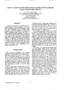
Thus, for each branch of the tree, the process yields a so-called placement of the QS, that is, an optimized position on the branch, along with a likelihood score for the whole tree. The likelihood scores for a QS are then transformed into probabilities, which quantify the uncertainty of placing the sequence on the respective branch [32, 33]. Those probabilities are called likelihood weight ratios (LWRs). The accumulated LWR sum over all branches for a single QS is 1.0. Figure 1 shows an example depicting the placements of one QS, including the respective LWRs. 0.06

67 68 69 70 71 72 73

0.02

0.01

0.05 0.03

0.1

0.02

0.01

0.7

Fig 1. Phylogenetic Placement of a Query Sequence. Each branch of the reference tree is tested as a potential insertion position, called a “placement” (blue dots). Note that placements have a specific position on their branch, due to the branch length optimization process. A probability of how likely it is that the sequence belongs to a specific branch is computed (numbers next to dots), which is called the likelihood weight ratio (LWR). The bold number (0.7) denotes the most probable placement of the sequence. This process is repeated for every QS. Note that the placement process is conducted independently for each QS. That is, for each QS, the algorithm starts calculating placements from scratch on the original RT. In summary, the result of a phylogenetic placement analysis is a mapping of the QSs in a sample to positions on the branches of the RT. Each such position, along with the corresponding LWR, is called a placement of the QS. When placing multiple samples, for instance, from different locations, typically, the same RT is used, in order to allow for comparisons of the phylogenetic composition of these samples. In this context, it sis important to consider how to properly normalize the samples. Normalization is required as the sample size (often also called library size), that is, the number of sequences per sample, can vary by several orders of magnitude, due to efficiency variations in the sequencing process or biases introduced by the amplification process. Selecting an appropriate normalization strategy constitutes a common problem in many metagenomic studies. The appropriateness depends on data characteristics [34], but also on the biological question asked. For example, estimating indices such as the species richness are often implemented via rarefaction and rarefaction curves [35], which however ignores a potentially large amount of the available valid data [36]. Furthermore, the specific type of input sequence data has to be taken into account for normalization: Biases induced by the amplification process can potentially be avoided if, instead of amplicons, data based on shotgun sequencing are used, such as mi tags [37]. Moreover, the sequences can be clustered prior to phylogenetic placement analysis, for instance, by constructing operational taxonomic units (OTUs) [38–41]. Analyses using OTUs focus on species diversity instead of simple abundances. OTU clustering substantially reduces the number of sequences, and hence greatly decreases the computational cost for placement analyses. Lastly, one may completely ignore the abundances (which are called “multiplicities” of placements) of the placed sequences, reads, or OTUs, and only be interested in their presence/absence

3/36

74 75 76 77 78 79 80 81 82 83 84 85 86 87 88 89 90 91 92 93 94 95 96 97 98 99 100


when comparing samples. Which of the above analysis strategies is deployed, depends on the specific design of the study and the research question at hand. The common challenge is that the number of sequences per sample differs, which affects most post-analysis methods. Before introducing our methods, we therefore explain how the necessary normalizations of sample sizes can be performed in the following. We also describe general techniques for interpreting and working with phylogenetic placement data. Some of these techniques have been used before as building blocks for methods like Edge PCA and Squash Clustering [23, 42].

Edge Masses

101 102 103 104 105 106 107 108 109

110

Methods that compare samples directly based on their sequences, such as the UniFrac distance [43, 44], can benefit from rarefaction [34]. However, in the context of phylogenetic placement, rarefaction is not necessary. Thus, more valid data can be kept. To this end, it is convenient to think of the reference tree as a graph (when exploiting graph properties of the tree, we refer to the branches of the tree as edges). Then, the per-branch LWRs for a single QS can be interpreted as mass points distributed over the edges of the RT, including their respective placement positions on the branches, cf. Figure 1. This implies that each QS has a total accumulated mass of 1.0 on the RT. We call this the mass interpretation of the placed QSs, and henceforth use mass and LWR interchangeably. The mass of an edge refers to the sum of the LWRs on that edge for all QSs of a sample, as shown in Figure 2(a). The total mass of a sample is then the sum over all edge masses, which is identical to the number of QSs in the sample. The key idea is to use the distribution of placement mass points over the edges of the RT to characterize a sample. This allows for normalizing samples of different size by scaling the total sample mass to unit mass 1.0. In other words, absolute abundances are converted into relative abundances. This way, rare species, which might have been removed by rarefaction, can be kept, as they only contribute a negligible mass to the branches into which they have been placed. This approach is analogous to using proportional values for methods based on OTU count tables, that is, scaling each sample/column of the table by its sum of OTU counts [34]. Most of the methods presented here use normalized samples, that is, they use relative abundances. As relative abundances are compositional data, certain caveats occur [45, 46], which we discuss where appropriate. When working with large numbers of QSs, the mass interpretation allows to further simplify and reduce the data: The masses on each edge of the tree can be quantized into b discrete bins, that is, each edge is divided into b intervals (or bins) of the corresponding branch length. All mass points on that edge are then accumulated into their respective nearest bin. The parameter b controls the resolution and accuracy of this approximation. In the extreme case b := 1, all masses on an edge are grouped into one single bin. This branch binning process drastically reduces the number of mass points that need to be stored and analyzed in several methods we present, while only inducing a negligible decrease in accuracy. As shown in Supplementary Table 1, branch binning can yield a speedup of up to 75% for post-analysis run-times. Furthermore, using masses allows to summarize a set of samples by annotating the RT with their average per-edge mass distribution. This procedure, also called squashing [23], sums over all sample masses per edge and then normalizes them once more to obtain unit mass for this resulting average tree. This normalized tree thereby summarizes the (sub-)set of samples it represents.

4/36

111 112 113 114 115 116 117 118 119 120 121 122 123 124 125 126 127 128 129 130 131 132 133 134 135 136 137 138 139 140 141 142 143 144 145 146 147 148


Edge Imbalances

149

So far, we have only considered the per-edge masses. Often, however, it is also of interest to “summarize” the mass of an entire clade. For example, sequences of the RT that represent species or strains might not provide sufficient phylogenetic signal for properly resolving the phylogenetic placement of short sequences [47]. In these cases, the placement mass of a sequence can be spread across different edges representing the same genus or species, thus blurring analyses based on per-edge masses. Instead, a clade-based summary can yield clearer analysis results. It can be computed by using the tree structure to appropriately transform the edge masses. Each edge splits the tree into two parts, of which only one contains the root (or top-level trifurcation) of the tree. For a given edge, its mass difference is then calculated by summing all masses in the root part of the tree and subtracting all masses in the other part, while ignoring the mass of the edge itself [23]. This difference is called the imbalance of the edge. It is usually normalized to represent unit total mass, as the absolute (not normalized) imbalance otherwise propagates the effects of differing sample sizes all across the tree. An example of the imbalance calculation is shown in Figure 2(a). The edge imbalance relates the masses on the two sides of an edge to each other. This implicitly captures the RT topology and reveals information about its clades. Furthermore, this transformation can also reveal differences in the placement mass distribution of nearby branches of the tree. This is in contrast to the KR distance, which yields low values for masses that are close to each other on the tree. An example that illustrates the different use cases for edge mass and edge imbalance metrics is shown in Figure 3. The edge masses and edge imbalances per sample can be summarized by two matrices, which we use for all further downstream edge- and clade-related analyses, respectively. In these matrices, each row corresponds to a sample, and each column to an edge of the RT. Note that these matrices can either store absolute or relative abundances, depending on whether the placement mass was normalized. Furthermore, many studies provide meta-data for their samples, for instance, the pH value or temperature of the samples’ environment. Such meta-data features can also be summarized in a per-sample matrix, where each column corresponds to one feature. The three matrices are shown in Figure 2(b). Quantitative meta-data features are the most suitable for our purposes, as they can be used to detect correlations with the placement mass distributions of samples. For example, Edge principal components analysis (Edge PCA) [23] is a method that utilizes the imbalance matrix to detect and visualize edges with a high heterogeneity of mass difference between samples. Edge PCA further allows to annotate its plots with meta-data variables, for instance, by coloring, thus establishing a connection between differences in samples and differences in their meta-data [14]. In the following, we propose several new techniques to analyze placement data and their associated meta-data.

Methods

150 151 152 153 154 155 156 157 158 159 160 161 162 163 164 165 166 167 168 169 170 171 172 173 174 175 176 177 178 179 180 181 182 183 184 185 186 187

188

In this section, we introduce novel methods for analyzing and visualizing the phylogenetic placement data of a set of environmental samples. Each such sample represents a geographical location, a body site, a point in time, etc. In the following, we represent a sample by the placement locations of its metagenomic QSs, including the respective per-branch LWRs. Furthermore, for a specific analysis, we assume the standard use case, that is, all placements were computed on the same fixed reference tree (RT) and reference alignment. We initially describe the methods. We then assess their application to real world data and their computational efficiency in Section Results and Discussion.

5/36

189 190 191 192 193 194 195 196 197


(a) (0.11 + 0.19 + 0.10 + 0.42 + 0.04 + 0.03) - (0.04 + 0.01) = 0.84

0.04 -0.68

0.03 0.97

0.06 0.84

0.10 0.30 0.11 0.89

0.42 0.58 0.19 0.81

0.04 0.96

0.01 0.99

Samples

(b) Edges

Edges

Features

Masses

Imbalances

Metadata

Fig 2. Edge Masses and Imbalances. (a) Reference tree where each edge is annotated with the normalized mass (first value, blue) and imbalance (second value, red) of the placements in a sample. The imbalance is the sum of masses on the root side of the edge minus the sum of the masses on the non-root side. The depicted tree is unrooted, hence, its top-level trifurcation (gray dot) is used as “root” node. An exemplary calculation of the imbalance is given at the top. Because terminal edges only have a root side, their imbalance is not informative. (b) The masses and imbalances for the edges of a sample constitute the rows of the first two matrices. The third matrix contains the available meta-data features for each sample. These matrices are used to calculate, for instance, the edge principal components or correlation coefficients.

Visualization

198

A first step in analyzing phylogenetic placement data is often to visualize them. For small samples, it is possible to mark individual placement locations on the RT, as offered for example by iTOL [48], or even to create a tree where the most probable placement per QS is attached as a new branch, as implemented in the guppy tool from the pplacer suite [17], RAxML-EPA [18, 49], and our tool gappa. For larger samples, one can alternatively display the per-edge placement mass, either by adjusting the line widths of the edges according to their mass, or by using a color scale, as offered in ggtree [50], guppy, and gappa. Using per-edge colors corresponds to binning all placement of an edge into one bin. For large datasets, the per-edge masses can vary by several orders of magnitude. In these cases, it is often preferable to use a logarithmic scaling, as shown in [11]. These simple visualizations directly depict the placement masses on the tree. When visualizing the accumulated masses of multiple samples at once, it is important to chose the appropriate normalization strategy for the task at hand. For example, if samples represent different locations, one might prefer to use normalized masses, as comparing relative abundances is common for this type of data. On the other hand, if samples from the same location are combined (e.g., from different points in time, or different size fractions), it might be preferable to use absolute abundances instead, so that the total number of sequences per sample can be visualized. The visualizations provide an overview of the species abundances over the tree. They

6/36

199 200 201 202 203 204 205 206 207 208 209 210 211 212 213 214 215 216 217 218


can be regarded as a more detailed version of classic abundance pie charts. When placing OTUs, or ignoring sequence abundances, the resulting visualizations depict species diversity. Moreover, these visualizations can be used to assess the quality of the RT. For example, placements into inner branches of the RT may indicate that appropriate reference sequences (i) have not been included or (ii) are simply not yet available. Here, we introduce visualization methods that highlight (i) regions of the tree with a high variance in their placement distribution (called Edge Dispersion), and (ii) regions with a high correlation to meta-data features (called Edge Correlation). Edge Dispersion

219 220 221 222 223 224 225 226 227

228

The Edge Dispersion is derived from the edge masses or edge imbalances matrix by calculating a measure of dispersion for each of the matrix columns, for example the standard deviation σ. Because each column corresponds to an edge, this information can be mapped back to the tree, and visualized, for instance, via color coding. This allows to examine which edges exhibit a high heterogeneity of placement masses across samples, and indicates which edges discriminate samples. As edge mass values can span many orders of magnitude, it might be necessary to scale the variance logarithmically. Often, one is more interested in the branches with high placement mass. In these cases, using the standard deviation or variance is appropriate, as they also indicate the mean mass per edge. On the other hand, by calculating the per-edge Index of Dispersion [51], that is, the variance-mean-ratio σ2/µ, differences on edges with little mass also become visible. As Edge Dispersion relates placement masses from different samples to each other, the choice of the normalization strategy is important. When using normalized masses, the magnitude of dispersion values needs to be cautiously interpreted [46]. The Edge Dispersion can also be calculated for edge imbalances. As edge imbalances are usually normalized to [−1.0, 1.0], their dispersion can be visualized directly without any further normalization steps. An example for an Edge Dispersion visualization is shown in Figure 3(a), and discussed in Section Visualization. Edge Correlation

229 230 231 232 233 234 235 236 237 238 239 240 241 242 243 244 245 246

247

In addition to the per-edge masses, the Edge Correlation further takes a specific meta-data feature into account, that is, a column of the meta-data matrix. The Edge Correlation is calculated as the correlation between each edge column and the feature column, for example by using the Pearson Correlation Coefficient or Spearman’s Rank Correlation Coefficient [51]. This yields a per-edge correlation of the placement masses or imbalances with the meta-data feature, and can again be visualized via color coding of the edges. It is inexpensive to calculate and hence scales well to large datasets. As typical correlation coefficients are within [−1.0, 1.0], there is again no need for further normalization. This yields a tree where edges or clades with either a high linear or monotonic correlation with the selected meta-data feature are highlighted. Figure 3(b) shows an example of this method. In contrast to Edge PCA [23] that can use meta-data features to annotate samples in its scatter plots, our Edge Correlation method directly represents the influence of a feature on the branches or clades of the tree. It can thus, for example, help to identify and visualize dependencies between species abundances and environmental factors such as temperature or nutrient levels. Again, the choice of normalization strategy is important to draw meaningful conclusions. However, the correlation is not calculated between samples or sequence abundances. Hence, even when using normalized samples, the pitfalls regarding correlations of compositional data [46] do not apply here.

7/36

248 249 250 251 252 253 254 255 256 257 258 259 260 261 262 263 264 265 266


Clustering

267

Given a set of metagenomic samples, one key question is how much they differ from each other. A common distance metric between microbial communities is the (weighted) UniFrac distance [43, 44]. It uses the fraction of unique and shared branch lengths between phylogenetic trees to determine their difference. UniFrac has been generalized and adapted to phylogenetic placements in form of the phylogenetic Kantorovich-Rubinstein (KR) distance [23, 42]. In other contexts, the KR distance is also called Wasserstein distance, Mallows distance, or Earth Mover’s distance [52–55]. The KR distance between two metagenomic samples is a metric that describes by at least how much the normalized mass distribution of one sample has to be moved across the RT to obtain the distribution of the other sample. The distance is symmetrical, and becomes larger the more mass needs to be moved, and the larger the respective displacement (moving distance) is. As the two samples being compared need to have equal masses, the KR distance operates on normalized samples; that is, it compares relative abundances. Given such a distance measure between samples, a fundamental task consists in clustering samples that are similar to each other. Standard linkage-based clustering methods like UPGMA [56–58] are solely based on the distances between samples, that is, they calculate the distances of clusters as a function of pairwise sample distances. Squash Clustering [14, 23] is a method that also takes into account the intrinsic structure of phylogenetic placement data. It uses the KR distance to perform agglomerative hierarchical clustering of samples. Instead of using pairwise sample distances, however, it merges (squashes) clusters of samples by calculating their average per-edge placement mass. Thus, in each step, it operates on the same type of data, that is, on mass distributions on the RT. This results in a hierarchical clustering tree that has meaningful, and hence interpretable, branch lengths. Phylogenetic k-means

Algorithm 1 Phylogenetic k-means

4: 5:

269 270 271 272 273 274 275 276 277 278 279 280 281 282 283 284 285 286 287 288 289 290 291 292

293

The number of tips in the resulting clustering tree obtained through Squash Clustering is equal to the number n of samples that are being clustered. Thus, for datasets with more than a few hundred samples, the clustering result becomes hard to inspect and interpret visually. We propose a variant of k-means clustering [59] to address this problem, which we call Phylogenetic k-means. It uses a similar approach as Squash Clustering, but yields a predefined number of k clusters. It is hence able to work with arbitrarily large datasets. Note that we are clustering samples here, instead of sequences [60]. We discuss choosing a reasonable value for k later. The underlying idea is to assign each of the n samples to one of k cluster centroids, where each centroid represents the average mass distribution of all samples assigned to it. Note that all samples and centroids are of the same data type, namely, they are mass distributions on a fixed RT. It is thus possible to calculate distances between samples and centroids, and to calculate their average mass distributions, as described earlier. Our implementation follows Lloyd’s algorithm [61], as shown in Algorithm 1.

1: 2: 3:

268

initialize k Centroids while not converged do assign each Sample to nearest Centroid update Centroids as mass averages of their Samples return Assignments and Centroids

8/36

294 295 296 297 298 299 300 301 302 303 304 305 306 307


By default, we use the k-means++ initialization algorithm [62] to obtain a set of k initial centroids. It works by subsequent random selection of samples to be used as initial centroids, until k centroids have been selected. In each step, the probability of selecting a sample is proportional to its squared distance to the nearest already selected sample. An alternative initialization is to select samples as initial clusters entirely at random. This is however more likely to yield sub-optimal clusterings [63]. Then, each sample is assigned to its nearest centroid, using the KR distance. Lastly, the centroids are updated to represent the average mass distribution of all samples that are currently assigned to them. This iterative process alternates between improving the assignments and the centroids. Thus, the main difference to normal k-means is the use of phylogenetic information: Instead of euclidean distances on vectors, we use the KR distance, and instead of averaging vectors to obtain centroids, we use the average mass distribution. The process is repeated until it converges, that is, the cluster assignments do not change any more, or until a maximum number of iterations have been executed. The second stopping criterion is added to avoid the super-polynomial worst case running time of k-means, which however almost never occurs in practice [64, 65]. The result of the algorithm is an assignment of each sample to one of the k clusters. As the algorithm relies on the KR distance, it clusters samples with similar relative abundances. The cluster centroids can be visualized as trees with a mass distribution, analogous to how Squash Clustering visualizes inner nodes of the clustering tree. That is, each centroid can be represented as the average mass distribution of the samples that were assigned to it. This allows to inspect the centroids and thus to interpret how the samples were clustered. Examples of this are shown in Supplementary Figure 6. The key question is how to select an appropriate k that reflects the number of “natural” clusters in the data. There exist various suggestions in the literature [66–71]; we assessed the Elbow method [66] as explained in Supplementary Figure 8, which is a straight forward method that yielded reasonable results for our test datasets. Additionally, for a quantitative evaluation of the clusterings, we used the k that arose from the number of distinct labels based on the available meta-data for the data. For example, the HMP samples are labeled with 18 distinct body sites, describing where each sample was taken from, see Figure 5. Algorithmic Improvements

308 309 310 311 312 313 314 315 316 317 318 319 320 321 322 323 324 325 326 327 328 329 330 331 332 333 334 335 336 337 338 339

340

In each assignment step of the algorithm, distances from all samples to all centroids are calculated, which has a time complexity of O(n · k). In order to accelerate this step, we can apply branch binning as introduced in Section Edge Masses. For the BV dataset, we found that even using just 2 bins per edge does not alter the cluster assignments. Branch binning reduces the number of mass points that have to be accessed in memory during KR distance calculations; however, the costs for tree traversals remain. Thus, we observed a maximal speedup of 75% when using one bin per branch, see Supplementary Table 1 for details. Furthermore, during the execution of the algorithm, empty clusters can occur, for example, if k is greater than the number of natural clusters in the data. Although this problem did not occur in our tests, we implemented the following solution: First, find the cluster with the highest variance. Then, choose the sample of that cluster that is furthest from its centroid, and assign it to the empty cluster instead. This process is repeated if multiple empty clusters occur at once.

9/36

341 342 343 344 345 346 347 348 349 350 351 352 353 354


Imbalance k-means

355

We further propose Imbalance k-means, which is a variant of k-means that makes use of the edge imbalance transformation, and thus also takes the clades of the tree into account. In order to quantify the difference in imbalances between two samples, we use the euclidean distance between their imbalance vectors (that is, rows of the imbalance matrix). This is a suitable distance measure, as the imbalances implicitly capture the tree topology as well as the placement mass distributions. As a consequence, the expensive tree traversals required for Phylogenetic k-means are not necessary here. The algorithm takes the edge imbalance matrix of normalized samples as input, as shown in Figure 2(b), and performs a standard euclidean k-means clustering following Lloyd’s algorithm. This variant of k-means tends to find clusters that are consistent with the results of Edge PCA, as both use the same input data as well as the same distance measure. Furthermore, as the method does not need to calculate KR distances, and thus does not involve tree traversals, it is several orders of magnitude faster than the Phylogenetic k-means. For example, on the HMP dataset, it runs in mere seconds, instead of several hours needed for Phylogenetic k-means; see Section Performance for details.

356 357 358 359 360 361 362 363 364 365 366 367 368 369 370 371

Results and Discussion

372

We used three real world datasets to evaluate our methods:

373

• Bacterial Vaginosis (BV) [14]. This small dataset was already analyzed with phylogenetic placement in the original publication. We used it as an example of an established study to compare our results to. It has 220 samples with a total of 15 060 unique sequences. • Tara Oceans (TO) [7, 24, 25]. This world-wide sequencing effort of the open oceans provides a rich set of meta-data, such as geographic location, temperature, and salinity. Unfortunately, the sample analysis for creating the official data repository is still ongoing. We thus were only able to use 370 samples with 27 697 007 unique sequences. • Human Microbiome Project (HMP) [12, 13]. This large data repository intends to characterize the human microbiota. It contains 9192 samples from different body sites with a total of 63 221 538 unique sequences. There is additional meta-data such as age and medical history, which is available upon special request. We only used the publicly available meta-data. Details of the datasets (download links, data statistics, data preprocessing, etc.) are provided in Supplementary Section Empirical Datasets. At the time of writing, about one year after we initially downloaded the data, the TO repository has grown to 1170 samples, while the HMP even published a second phase and now comprises 23 666 samples of the 16S region. This further emphasizes the need for scalable methods to analyze such data. These datasets represent a wide range of environments, number of samples, and sequence lengths. We use them to evaluate our methods and to exemplify which method is applicable to what kind of data. To this end, the sequences of the datasets were placed on appropriate phylogenetic RTs as explained in the supplement, in order to obtain phylogenetic placements that our methods can be applied to. In the following, we present the respective results, and also compare our methods to other methods where applicable. As the amount and type of available meta-data differs for each

10/36

374 375 376 377

378 379 380 381 382

383 384 385 386 387

388 389 390 391 392 393 394 395 396 397 398 399 400


dataset, we could not apply all methods to all datasets. Lastly, we also report the run-time performance of our methods on these data.

401 402

Visualization

403

BV Dataset

404

We re-analyzed the BV dataset by inferring a tree from the original reference sequence set and conducting phylogenetic placement of the 220 samples. The characteristics of this dataset were already explored in [14] and [23]. We use it here to give exemplary interpretations of our Edge Dispersion and Edge Correlation methods, and to evaluate them in comparison to existing methods. Figure 3 shows our novel visualizations of the BV dataset. Edge Dispersion is shown in Figure 3(a), while Figure 3(b) shows Edge Correlation with the so-called Nugent score. The Nugent score [72] is a clinical standard for the diagnosis of Bacterial Vaginosis, ranging from 0 (healthy) to 10 (severe illness). The connection between the Nugent score and the abundance of placements on particular edges was already explored in [23], but only visualized indirectly (i.e., not on the RT itself). For example, Figure 6 of the original study plots the first two Edge PCA components colorized by the Nugent score. We recalculated this figure for comparison in Supplementary Figure 5(i). In contrast, our Edge Correlation measure directly reveals the connection between Nugent score and placements on the reference tree: The clade on the left hand side of the tree, to which the red and orange branches lead to, are Lactobacillus iners and Lactobacillus crispatus, respectively, which were identified in [14] to be associated with a healthy vaginal microbiome. Thus, their presence in a sample is anti-correlated with the Nugent score, which is lower for healthy subjects. The branches leading to this clade are hence colored in red. On the other hand, there are several other clades that exhibit a positive correlation with the Nugent score, that is, were green and blue paths lead to in the Figure, again a finding already reported in [14]. (b)

(a)

172

1.0

100

10

≤1

0.0

-1.0

Fig 3. Examples of Edge Dispersion and Edge Correlation. We applied our novel visualization methods to the BV dataset to compare them to the existing examinations of the data. (a) Edge Dispersion, measured as the standard deviation of the edge masses across samples, logarithmically scaled. (b) Edge Correlation, in form of Spearman’s Rank Correlation Coefficient between the edge imbalances and the Nugent score. Tip edges are gray, because they do not have a meaningful imbalance. This example also shows the characteristics of edge masses and edge imbalances: The former highlights individual edges, the latter paths to clades.

11/36

405 406 407 408 409 410 411 412 413 414 415 416 417 418 419 420 421 422 423 424 425 426


Both trees in Figure 3 highlight the same parts of the tree: The dark branches with high deviation in (a) represent clades attached to either highly correlated (blue) or anti-correlated (red) paths (b). This indicates that edges that have a high dispersion also vary between samples of different Nugent score. We further compared our methods to the visualization of Edge PCA components on the reference tree. To this end, we recalculated Figures 4 and 5 of [23], and visualized them with our color scheme in Supplementary Figure 3 for ease of comparison. They show the first two components of Edge PCA, mapped back to the RT. The first component reveals that the Lactobacillus clade represents the axis with the highest heterogeneity across samples, while the second componentfurther distinguishes between the two aforementioned clades within Lactobacillus. Edge Correlation also highlights the Lactobacillus clade as shown in Figure 3(b), but does not distinguish further between its sub-clades. This is because a high Nugent score is associated with a high abundance of placements in either of the two relevant Lactobacillus clades. Further examples of variants of Edge Dispersion and Edge Correlation on this dataset are shown in Supplementary Figures 1 and 2. We also conducted Edge Correlation using Amsel’s criteria [73] and the vaginal pH value (data not shown), both of which were used in [14] as additional indicators of Bacterial Vaginosis. We again found similar correlations compared to the Nugent score. Tara Oceans Dataset

427 428 429 430 431 432 433 434 435 436 437 438 439 440 441 442 443 444 445

446

We analyzed the TO dataset to provide further exemplary use cases for our visualization methods. To this end, we used the unconstrained Eukaryota RT with 2059 taxa as provided by our Automatic Reference Tree method [26]. The meta-data features of this dataset that best lend themselves to our methods are the sensor values for chlorophyll, nitrate, and oxygen concentration, as well as the salinity and temperature of the water samples. Other available meta-data features such as longitude and latitude are available, but would require more involved methods. This is because geographical coordinates yield pairwise distances between samples, whose integration into our correlation analysis methods is challenging. The Edge Correlation of the 370 samples with the nitrate concentration, the salinity, the chlorophyll concentration, and the water temperature are shown in Supplementary Figure 4. We selected the diatoms and the animals as two exemplary clades for closer examination of the results. In particular, the diatoms show a high correlation with the nitrate concentration, as well as an anti-correlation with salinity, which represent well-known relationships [74, 75]. See Supplementary Figure 4 for details. These findings indicate that the method is able to identify known relationships. It will therefore also be useful to investigate or discover insights of novel relationships between sequence abundances and environmental parameters. Performance

447 448 449 450 451 452 453 454 455 456 457 458 459 460 461 462 463 464

465

Both methods (Edge Dispersion and Edge Correlation) are computationally inexpensive, and thus applicable to large datasets. The calculation of the above visualizations took about 30 s each, which were mainly required for reading in the data. Furthermore, in order to scale to large datasets, we reimplemented Edge PCA, which was originally implemented as a command in the guppy program [17]. For the BV dataset with 220 samples, guppy required 9 min and used 2.2 GB of memory, while our implementation only required 33 s on a single core, using less than 600 MB of main memory. For the HMP dataset, as it is only single-threaded, guppy took 11 days and 75.1 GB memory, while our implementation needed 7.5 min on 16 cores and used 43.5 GB memory.

12/36

466 467 468 469 470 471 472 473 474


Clustering

475

We now evaluate our Phylogenetic k-means clustering (which uses edge masses and KR distances) and Imbalance k-means clustering (which uses edge imbalances and euclidean distances) methods in terms of their clustering accuracy. We used the BV as an example of a small dataset to which methods such as Squash Clustering [23] are still applicable, and the HMP dataset to showcase that our methods scale to datasets that are too large for existing methods. BV Dataset

476 477 478 479 480 481

482

We again use the re-analyzed BV dataset to test whether our methods work as expected, by comparing them to the existing analysis of the data in [14] and [23]. To this end, we ran both Phylogenetic k-means and Imbalance k-means on the BV dataset. We chose k := 3, inspired by the findings of [14]. They distinguish between subjects affected by Bacterial Vaginosis and healthy subjects, and further separate the healthy ones into two categories depending on the dominating clade in the vaginal microbiome, which is either Lactobacillus iners or Lactobacillus crispatus. Any choice of k > 3 would simply result in smaller, more fine-grained clusters, but not change the general findings of these experiments. An evaluation of the number of clusters using the Elbow method is shown in Supplementary Figure 8. We furthermore conducted Squash Clustering and Edge PCA on the dataset, thereby reproducing previous results, in order to allow for a direct comparison between the methods, see Figure 4. The figure shows the results of Squash Clustering, Edge PCA, and two alternative dimensionality reduction methods, colorized by the cluster assignments PKM of Phylogenetic k-means (in red, green, and blue) and IKM of the Imbalance k-means (in purple, orange, and gray), respectively. We use two different color sets for the two methods, in order to make them distinguishable at first glance. Note that the mapping of colors to clusters is arbitrary and depends on the random initialization of the algorithm. As can be seen in Figure 4(a), Squash Clustering as well as Phylogenetic k-means can distinguish healthy subjects from those affected by Bacterial Vaginosis. Healthy subjects constitute the lower part of the cluster tree. They have shorter branches between each other, indicating the smaller KR distance between them, which is a result of the dominance of Lactobacillus in healthy subjects. The same clusters are found by Phylogenetic k-means: As it uses the KR distance, it assigns all healthy subjects with short cluster tree branches to one cluster (shown in red). The green and blue clusters are mostly the subjects affected by the disease. The distinguishing features between the green and the blue cluster are not apparent in the Squash cluster tree. This can however be seen in Figure 4(c), which shows a Multidimensional scaling (MDS) plot of the pairwise KR distances between the samples. MDS [51, 77, 78] is a dimensionality reduction method that can be used for visualizing levels of similarity between data points. Given a pairwise distance matrix, it finds an embedding into lower dimensions (in this case, 2 dimensions) that preserves higher dimensional distances as well as possible. Here, the red cluster forms a dense region, which is in agreement with its short branch lengths in the cluster tree. At the same time, the green and blue cluster are separated in the MDS plot, but form a coherent region of low density, indicating that k := 3 might be too large with Phylogenetic k-means on this dataset. That is, the actual clustering just distinguishes healthy from sick patients (Supplementary Figure 8). A similar visualization of the pairwise KR distances is shown in Figure 4(d). It is a recalculation of Figure 4 in the preprint [76], which did not appear in the final published version [23]. The figure shows a standard Principal Components Analysis (PCA) [51, 78] applied to the distance matrix by interpreting it as a data

13/36

483 484 485 486 487 488 489 490 491 492 493 494 495 496 497 498 499 500 501 502 503 504 505 506 507 508 509 510 511 512 513 514 515 516 517 518 519 520 521 522 523 524


(b)

(c)

MDS2

(a)

MDS1

PC2

(d)

PC1

EdgePC2

(e)

PKM - Cluster Assignment with Phylogenetic k-means: red green blue

IKM - Cluster Assignment with Imbalance k-means: purple orange gray

EdgePC1

Fig 4. Comparison of k-means clustering to Squash Clustering and Edge PCA. We applied our variants of the k-means clustering method to the BV dataset in order to compare them to existing methods. See [14] for details of the dataset and its interpretation. We chose k := 3, as this best fits the features of the dataset. For each sample, we obtained two cluster assignments: First, by using Phylogenetic k-means, we obtained the cluster assignment PKM. Second, by using Imbalance k-means, we obtained assignment IKM. In each subfigure, the 220 samples are represented by colored circles: red, green, and blue show the cluster assignments PKM, while purple, orange, and gray show the cluster assignments IKM. (a) Hierarchical cluster tree of the samples, using Squash Clustering. The tree is a recalculation of Figure 1(A) of [14]. Each leaf represents a sample; branch lengths are KR distances. We added color coding for the samples, using PKM. The lower half of red samples are mostly healthy subjects, while the green and blue upper half are patients affected by Bacterial Vaginosis. (b) The same tree, but annotated by IKM. The tree is flipped horizontally for ease of comparison. The healthy subjects are split into two sub-classes, discriminated by the dominating species in their vaginal microbiome: orange and purple represent samples were Lactobacillus iners and Lactobacillus crispatus dominate the microbiome, respectively. The patients mostly affected by BV are clustered in gray. (c) Multidimensional scaling using the pairwise KR distance matrix of the samples, and colored by PKM. (d) Principal component analysis applied to the distance matrix by interpreting it as a data matrix. This is a recalculation of Figure 4 of [76], but colored by PKM. (e) Edge PCA applied to the samples, which is a recalculation of Figure 3 of [76], but colored by IKM. matrix, and was previously used to motivate Edge PCA. However, although it is mathematically sound, the direct application of PCA to a distance matrix lacks a simple interpretation. Again, the red cluster is clearly separated from the rest, but this time, the distinction between the green and the blue cluster is not as apparent. In Figure 4(b), we compare Squash Clustering to Imbalance k-means. Here, the

14/36

525 526 527 528 529


distinction between the two Lactobacillus clades can be seen by the purple and orange cluster assignments. The cluster tree also separates those clusters into clades. The separate small group of orange samples above the purple clade is an artifact of the tree ladderization. The diseased subjects are all assigned to the gray cluster, represented by the upper half of the cluster tree. It is apparent that both methods separate the same samples from each other. Lastly, Figure 4(e) compares Imbalance k-means to Edge PCA. The plot is a recalculation of Figure 3 of [76], which also appeared in Figure 6 in [23] and Figure 3 in [14], but colored using our cluster assignments. Because both methods work on edge imbalances, they group the data in the same way, that is, they clearly separate the two healthy groups and the diseased one from each other. Edge PCA forms a plot with three corners, which are colored by the three Imbalance k-means cluster assignments. In Supplementary Figure 5, we report more details of the comparison of our k-means variants to the dimensionality reduction methods used here. Furthermore, examples visualizations of the cluster centroids are shown in Supplementary Figure 6, which further supports that our methods yield results that are in agreement with existing methods. HMP Dataset

530 531 532 533 534 535 536 537 538 539 540 541 542 543 544 545 546

547

The HMP dataset is used here as an example to show that our method scales to large datasets. To this end, we used the unconstrained Bacteria RT with 1914 taxa as provided by our Automatic Reference Tree method [26]. The tree represents a broad taxonomic range of Bacteria, that is, the sequences were not explicitly selected for the HMP dataset, in order to test the robustness of our clustering methods. We then placed the 9192 samples of the HMP dataset with a total of 118 701 818 sequences on that tree, and calculated Phylogenetic and Imbalance k-means on the samples. The freely available meta-data for the HMP dataset labels each sample by the body site were it was taken from. As there are 18 different body site labels, we used k := 18. The result is shown in Figure 5. Furthermore, in Supplementary Figure 7, we show a clustering of this dataset into k := 8 broader body site regions to exemplify the effects of using different values of k. This is further explored by using the Elbow method as shown in Supplementary Figure 8. Ideally, all samples from one body site would be assigned to the same cluster, hence forming a diagonal on the plot. However, as there are several nearby body sites, which share a large fraction of their microbiome [12], we do not expect a perfect clustering. Furthermore, we used a broad reference tree that might not be able to resolve details in some clades. Nonetheless, the clustering is reasonable, which indicates a robustness against the exact choice of reference taxa, and can thus by used for distinguishing among samples. For example, stool and vaginal samples are clearly clustered. Furthermore, the sites that are on the surface of the body (ear, nose, and arm) also mostly form two blocks of cluster columns. Performance

548 549 550 551 552 553 554 555 556 557 558 559 560 561 562 563 564 565 566 567 568 569

570

The complexity of Phylogenetic k-means is in O(k · i · n · e), with k clusters, i iterations, and n samples, and e being the number of tree edges, which corresponds to the number of dimensions in standard euclidean k-means. As the centroids are randomly initialized, the number of iterations can vary; in our tests, it was mostly below 100. For the BV dataset with 220 samples and a reference tree with 1590 edges, using k := 3, our implementation ran 9 iterations, needing 35 s and 730 MB of main memory on a single core. For the HMP dataset with 9192 samples and 3824 edges, we used k := 18, which took 46 iterations and ran in 2.7 h on 16 cores, using 48 GB memory.

15/36

571 572 573 574 575 576 577 578


Body Site Region Stool Stool Saliva Saliva Tongue Dorsum Mouth (back) Throat Mouth (back) Palatine Tonsils Mouth (back) Attached Keratinized Gingiva Mouth (front) Hard Palate Mouth (front) Buccal Mucosa Mouth (front) Subgingival Plaque Plaque Supragingival Plaque Plaque Left Antecubital Fossa Arm Right Antecubital Fossa Arm Anterior Nares Nose Left Retroauricular Crease Ear Right Retroauricular Crease Ear Vaginal Introitus Vagina Mid Vagina Vagina Posterior Fornix Vagina

(a) Phylogenetic k-means

(b) Imbalance k-means

Clusters

Clusters

Fig 5. k-means cluster assignments of the HMP dataset with k := 18. Here, we show the cluster assignments as yielded by Phylogenetic k-means (a) and Imbalance k-means (b) of the HMP dataset. We used k := 18, which is the number of body site labels in the dataset, in order to compare the clusterings to this “ground truth”. Each row represents a body site; each column one of the 18 clusters found by the algorithm. The color values indicate how many samples of a body site were assigned to each cluster. Similar body sites are clearly grouped together in coherent blocks, indicated by darker colors. For example, the stool samples were split into two clusters (topmost row), while the three vaginal sites were all put into one cluster (rightmost column). However, the algorithm cannot always distinguish between nearby sites, as can be seen from the fuzziness of the clusters of oral samples. This might be caused by our broad reference tree, and could potentially be resolved by using a tree more specialized for the data/region (not tested). Lastly, the figure also lists how the body site labels were aggregated into regions as used in Supplementary Figure 7. Although the plots of the two k-means variants generally exhibit similar characteristics, there are some differences. For example, the samples from the body surface (ear, nose, arm) form two relatively dense clusters (columns) in (a), whereas those sites are spread across four of five clusters in (b). On the other hand, the mouth samples are more densely clustered in (b).

16/36


In contrast to this, Imbalance k-means does not need to conduct any expensive tree traversals, and instead operates on compact vectors, using euclidean distances. It is hence several orders of magnitude faster than Phylogenetic k-means. For example, using again k := 18 for the HMP dataset, the algorithm executed 75 iterations in 2 s. It is thus also applicable to extremely large datasets. Furthermore, as the KR distance is used in Phylogenetic k-means as well as other methods such as Squash Clustering, our implementation is highly optimized and outperforms the existing implementation in guppy [17] by orders of magnitude (see below for details). The KR distance between two samples has a linear computational complexity in both the number of QSs and the tree size. As a test case, we computed the pairwise distance matrix between sets of samples. Calculating this matrix is quadratic in the number of samples, and is thus expensive for large datasets. For example, in order to calculate the matrix for the BV dataset with 220 samples, guppy can only use a single core and required 86 min. Our KR distance implementation in genesis is faster and also supports multiple cores. It only needed 90 s on a single core; almost half of this time is used for reading input files. When using 32 cores, the matrix calculation itself only took 8 s. This allows to process larger datasets: The distance matrix of the HMP dataset with 9192 samples placed on a tree with 3824 branches for instance took less than 10 h to calculate using 16 cores in genesis. In contrast, guppy needed 43 days for this dataset. Lastly, branch binning can be used to achieve additional speedups, as shown in Supplementary Table 1.

Conclusion

579 580 581 582 583 584 585 586 587 588 589 590 591 592 593 594 595 596 597 598 599

600

We presented novel, scalable methods to analyze and visualize phylogenetic placements. Edge Dispersion highlights branches of the phylogenetic tree that exhibit variations in the number of placements, and thus allows to identify regions of the tree with a high placement heterogeneity. Edge Correlation additionally takes meta-data features into account, and identifies branches of the tree that correlate with quantitative features, such as the temperature or the pH value of the environmental samples. These methods complement existing methods such as Edge PCA, and are data exploration tools that can help unravel new patterns in phylogenetic placement data. The variants of the methods presented here are hence best used in combination with each other. Furthermore, we presented adapted variants of the k-means method, which exploit the structure of phylogenetic placement data to identify clusters of environmental samples. The method builds upon ideas such as Squash Clustering and can be applied to substantially larger datasets, as it uses a pre-defined number of clusters. For future exploration, other forms of cluster analyses could be extended to work on phylogenetic placement data, for example, soft k-means clustering [79, 80] or density-based methods [81]. The main challenge when adopting such methods consists in making them phylogeny-aware, that is, to use mass distributions on trees instead of the typical Rn vectors. The presented methods take either the edge masses or the edge imbalances as input, and can hence analyze different aspects of the placements. While edge masses reveal information about single branches, edge imbalances take entire reference tree clades into account. Depending on the task at hand, either of them might be preferable, although they generally exhibit similar properties. We emphasize again the importance of appropriately normalizing the sample sizes as required. That is, depending on the type of sequence data, using either absolute or relative abundances is critical to allow for meaningful interpretation of the results. We tested our novel methods on three real-world datasets and gave exemplary interpretations of the results. We further showed that these results are consistent with

17/36

601 602 603 604 605 606 607 608 609 610 611 612 613 614 615 616 617 618 619 620 621 622 623 624 625 626 627 628


existing methods as well as empirical biological knowledge. Hence, our methods will also be useful to unravel new, unexplored relationships in metagenomic data. The methods are computationally inexpensive, and are thus, as we have demonstrated, applicable to large datasets. They are implemented in our tool gappa, which is freely available under GPLv3 at http://github.com/lczech/gappa. Furthermore, scripts, data and other tools used for the tests and figures presented here are available at http://github.com/lczech/placement-methods-paper.

Acknowledgments

629 630 631 632 633 634 635

636

This work was financially supported by the Klaus Tschira Stiftung gGmbH in Heidelberg, Germany. We thank S. Srinivasan and E. Matsen for providing the Bacterial Vaginosis dataset [14] and for helping us understanding their methods and implementations. We also thank M. Dunthorn, L. Rubinat, C. Berney, L. Guidi, G. Lentendu, A. Kozlov, and P. Barbera for their feedback on our methods and this manuscript.

18/36

637 638 639 640 641 642


Supporting Information

643

1

644

Empirical Datasets

The analyses and figures presented here were conducted on distinct reference alignments and trees. Firstly, for the BV dataset, we used the original set of reference sequences, and re-inferred a tree on them. Secondly, for the TO and HMP datasets, we used our Automatic Reference Tree (ART) method [26] to construct sets of suitable reference sequences from the Silva database [82, 83]. We used the 90% threshold consensus sequences; see [26] for details. For all analyses, we used the following software setup: Unconstrained maximum likelihood trees were inferred using RAxML v8.2.8 [49]. For aligning reads against reference alignments and reference trees, we used a custom MPI wrapper for PaPaRa 2.0 [27, 28], which is available at [84]. We then applied the chunkify procedure as explained in [26] to split the sequences into chunks of unique sequences prior to conducting the phylogenetic placement, in order to minimize processing time. Phylogenetic placement was conducted using EPA-ng [19], which is a faster and more scalable phylogenetic placement implementation than RAxML-EPA [18] and pplacer [17]. Lastly, given the per-chunk placement files produced by EPA-ng, we executed the unchunkify procedure of [26] to obtain per-sample placement files. These subsequently served as the input data for the methods presented here.

1.1

Bacterial Vaginosis

646 647 648 649 650 651 652 653 654 655 656 657 658 659 660 661

662

We used the Bacterial Vaginosis dataset [14] in order to compare our novel methods to existing ones such as Edge PCA and Squash Clustering [23, 42]. The dataset contains metabarcoding sequences of the vaginal microbiome of 220 women, and was kindly provided by Sujatha Srinivasan. This small dataset with a total of 426 612 query sequences, thereof 15 060 unique, was already analyzed with phylogenetic placement methods in the original publication. We re-inferred the reference tree of the original publication using the original alignment, which contains 797 reference sequences specifically selected to represent the vaginal microbiome. As the query sequences were already prepared, no further preprocessing was applied prior to phylogenetic placement. The available per-sample quantitative meta-data for this dataset comprises the Nugent score [72], the value of Amsel’s criteria [73], and the vaginal pH value. We used all three meta-data types in our analyses.

1.2

645

Tara Oceans

663 664 665 666 667 668 669 670 671 672 673 674

675

The Tara Oceans (TO) dataset [7, 24, 25] that we used here contains amplicon sequences of protists, and is available at https://www.ebi.ac.uk/ena/data/view/PRJEB6610. At the time of download, there were 370 samples available with a total of 49 023 231 sequences. As the available data are raw fastq files, we followed [85] to generate cleaned per-sample fasta files. For this, we used our tool PEAR [86] to merge the paired-end reads; cutadapt [87] for trimming tags as well as forward and reverse primers; and vsearch [41] for filtering erroneous sequences and generating per-sample fasta files. We filtered out sequences below 95 bps and above 150 bps, to remove potentially erroneous sequences. No further preprocessing (such as chimera detection) was applied. This resulted in a total of 48 036 019 sequences, thereof 27 697 007 unique. The sequences were then used for phylogenetic placement as explained above. We placed the sequences on the unconstrained Eukaryota reference tree obtained via our ART method [26], which comprises 2059 taxa, thereof 1795 eukaryotic sequences. The remaining 264 taxa are Archaea and Bacteria, and were included as a broad outgroup.

19/36

676 677 678 679 680 681 682 683 684 685 686 687 688 689


The TO dataset has a rich variety of per-sample meta-data features; in the context of this paper, we mainly focus on quantitative features such as temperature, salinity, as well as oxygen, nitrate and chlorophyll content of the water. Furthermore, each sample has meta-data features indicating the date, longitude and latitude, depth, etc. of the sampling location. This data might be interesting for further correlation analyses based on geographical information. We did not use them here, as for example longitude and latitude would require a more involved method that also accounts for, e.g., ocean currents. Furthermore, geographical coordinates yield pairwise distances between samples, which are not readily usable with our correlation analysis. Lastly, in order to use features such as the date, that is, in order to analyze samples over time, the same sampling locations would need to be visited at different times during the year, which is not the case for the Tara Oceans expedition.

1.3

Human Microbiome Project

691 692 693 694 695 696 697 698 699 700 701

702

We used the Human Microbiome Project (HMP) dataset [12, 13] for testing the scalability of our methods. In particular, we used the “HM16STR” data of the initial phase “HMP1”, which are available from http://www.hmpdacc.org/hmp/. The dataset consists of trimmed 16S rRNA sequences of the V1V3, V3V5, and V6V9 regions. The data are further divided into a “by_sample” set and a “healthy” set, which we merged in order to obtain one large dataset, with a total of 9811 samples. We then removed 10 samples that were larger than 70 MB as well as 605 samples that had fewer than 1500 sequences, because we considered them as defective or unreliable outliers. Finally, we also removed 2 samples that did not have a valid body site label assigned to them. This resulted in a set of 9192 samples containing a total of 118 702 967 sequences with an average length of 413 bps. From these samples, sequences with a length of less than 150 bps as well as sequences longer than 540 bps were removed, as we considered them potentially erroneous. No further preprocessing (such as chimera detection) was applied. This resulted in a total of 116 520 289 sequences, of which 63 221 538 were unique. We then used the unconstrained Bacteria tree of our ART method [26] for phylogenetic placement. The tree comprises 1914 taxa, thereof 1797 bacterial sequences. The remaining 117 taxa are Archaea and Eukaryota, and were included as a broad outgroup. Each sample is labeled with one of 18 human body site locations where it was sampled. This is the only publicly available meta-data feature.

2

690

Pipeline and Implementation

703 704 705 706 707 708 709 710 711 712 713 714 715 716 717 718 719 720 721

722

The methods described here are implemented in our tool gappa, which is freely available under GPLv3 at http://github.com/lczech/gappa. gappa internally uses our C++ library genesis, which offers functionality for working with phylogenies and phylogenetic placement data, and also contains methods to work with taxonomies, sequences and many other data types. genesis is also freely available under GPLv3 at http://github.com/lczech/genesis. gappa offers a command line interface for conducting typical tasks when working with phylogenetic placements. The methods that we described here are implemented via the following sub-commands: • dispersion: The command takes a set of jplace files (called samples), and calculates and visualizes the Edge Dispersion per edge of the reference tree. • correlation: The command takes a set of jplace samples, as well as a table containing metadata features for each sample. It then calculates and visualizes the Edge Correlation with the metadata features per edge of the reference tree.

20/36

723 724 725 726 727 728 729 730 731

732 733

734 735 736


• phylogenetic-kmeans and imbalance-kmeans: Performs k-means clustering of a set of jplace files according to our methods. • squash and edgepca: Reimplementations of the two existing methods [23, 42]. These are the gappa commands that are relevant for this paper. The tool also offers additional commands that are useful for phylogenetic placement data, such as visualization or filtering. At the time of writing this manuscript, gappa is under active development, with more functions planned in the near future. Lastly, we provide prototype implementations, scripts, data, and other tools used for the tests and figures in this paper at http://github.com/lczech/placement-methods-paper.

21/36

737 738

739

740 741 742 743 744 745


S1 Table. Effect of Branch Binning on the KR Distance of the HMP Dataset. Here we show the effect of per-branch placement binning on the run-time and on the resulting relative error when calculating the pairwise KR distance matrix between samples, by example of the Human Microbiome Project (HMP) [12, 13] dataset. Because of the size of the dataset (9192 samples) and reference tree (1914 taxa), we executed this evaluation in parallel on 16 cores. The first row shows the baseline performance, that is, without binning. When using fewer bins per branch, the run-time decreases, at the cost of slightly increasing the average relative error. Still, even when compressing the placement masses into only one bin per branch (that is, just using per-branch masses), the average relative error of the KR distances is around 1%, which is acceptable for most applications. However, considering that the run-time savings are not substantially better for a low number of bins, we recommend using a relatively large number of bins, e.g., 32 or more. This is because run-times of KR distance calculations also depend on other effects such as the necessary repeated tree traversals. We also conducted these tests on the BV dataset (data not shown), were the relative error is even smaller. Bins

Time (h:mm)

Speedup

Relative ∆

256 128 64 32 16 8 4 2 1

9:46 6:58 6:39 6:30 6:25 6:13 6:08 6:07 6:04 5:35

1.00 1.40 1.47 1.50 1.52 1.57 1.59 1.60 1.61 1.75

0.000000 0.000008 0.000015 0.000035 0.000124 0.000272 0.000669 0.002747 0.004284 0.011585

22/36


(a) Edge Masses, Standard Deviation

(b) Edge Masses, Standard Deviation, Log Scaled

172

172

150

100

100 10

50

≤1

0

(c) Edge Masses, Index of Dispersion, Log Scaled

(d) Edge Imbalances, Standard Deviation

1,000

0.9 0.8

100

0.6 0.4

10 0.2 ≤1

0

S1 Figure. Examples of variants of Edge Dispersion. We re-analyzed the BV dataset to show variants of our Edge Dispersion method. All subfigures highlight the same branches and clades as found by other methods such as Edge PCA. The method is useful as a first exploratory tool to detect placement heterogeneity across samples. In contrast to Edge Correlation, it can however not explain the reasons of heterogeneity. Subfigure (a) shows the standard deviation of the absolute edge masses, without any further processing. It is striking that one outlier, marked with an arrow, is dominating, thus hiding the values on less variable edges. This outlier occurs at the species Prevotella bivia in one of the 220 samples, where 2781 out of 2782 sequences in the sample have placement mass on that branch. Upon close examination, this outlier can also be seen in Figure 1D of [14], but is less apparent there. Subfigure (b) is identical to Figure 3(a) of the main text and shows the standard deviation again, but this time using logarithmic scaling, thus revealing more details on the edges with lower placement mass variance. Furthermore, when comparing it to Supplementary Figure 2(c), we see that the same clades that exhibit a high correlation or anti-correlation with meta-data there are also highlighted here. Subfigure (c) shows the Index of Dispersion of the edge masses, that is, the variance normalized by the mean. Hence, edges with a higher number of placements are also allowed to have a higher variance. We again use a logarithmic scale because of the outlier. The figure reveals more details on the edges with lower variance, highlighted in medium green colors. Subfigure (d) shows the standard deviation of edge imbalances. Because we used imbalances of unit mass samples, the values are already normalized. The path to the Lactobacillus clade is again clearly visible, indicating that the placement mass in this clade has a high variance across samples. Note that imbalances can be negative; thus, the Index of Dispersion is not applicable to them. 23/36


Edge Masses

Edge Imbalances (b)

(c)

(d)

Spearman's rank correlation coeﬃcient

Pearson correlation coeﬃcient

(a)

1.0

0.0

-1.0

S2 Figure. Examples of variants of Edge Correlation. We again use the BV dataset, and show the correlation of edge masses and imbalances with the Nugent score. The Nugent score measures the severeness of Bacterial Vaginosis, and ranges from 0 for healthy subjects to 10 for heavily affected patients. Subfigures (a) and (b) use the Pearson Correlation Coefficient, that is, they show the linear correlation with the meta-data feature, while subfigures (c) and (d) use Spearman’s Rank Correlation Coefficient and thus show monotonic correlations. Subfigure (d) is identical to Figure 3(b) of the main text. All subfigures show red edges or red paths at the Lactobacillus clade. This indicates that presence of placements in this clade is anti-correlated with the Nugent score, which is consistent with the findings of [14] and [23]. In other words, presence of Lactobacillus correlates with a healthy vaginal microbiome. On the other hand, blue and green edges, which indicate positive correlation, are indicative of edges that correlate to Bacterial Vaginosis. The extent of correlation is larger for Spearman’s Coefficient, indicating that the correlation is monotonic, but not strictly linear.

24/36


(a)

(b)

0.3 0.2 0.2 0.1 0.0 -0.1

0.1 0.0 -0.1 -0.2

-0.2 -0.3

S3 Figure. Recalculation of the Edge PCA tree visualization. Subfigures (a) and (b) are recalculations of Figures 4 and 5 of [23], respectively. However, we show them here in our coloring scheme in order to facilitate comparison with other figures. The original publication instead uses two colors for a positive and a negative sign of the principal components, and branch width to show their magnitude. Note that the actual sign is arbitrary, as it is derived from principal components. The figure shows the first two Edge PCA components, visualized on the reference tree. This form of visualization is useful to interpret results such as the Edge PCA projection plot as shown in Figure 4(e) of the main text. It reveals which edges are mainly responsible for separating the samples into the PCA dimensions. Here, the first principal component in (a) indicates that the main PCA axis separates samples based on the presence of placements in the Lactobacillus clade, which is what the blue and green path leads to. The second component in (b) then further distinguishes between two species in this clade, namely Lactobacillus iners and Lactobacillus crispatus.

25/36


(a) Nitrate concentration

(b) Salinity Diatoms

Diatoms

Animals

(c) Chlorophyll concentration

(d) Temperature Diatoms

1.0

0.0

Animals -1.0

S4 Figure. Examples of Edge Correlation using Tara Oceans samples. The figure shows the correlation of Tara Oceans sequence placements with (a) the nitrate, (b) the salinity, (c) the chlorophyll, and (d) the temperature sensor data of each sample. The sensor values range from −2.2 to 33.1 µmol/l (nitrate), from 33.2 to 40.2 psu (salt), from −0.02 to 1.55 mg/m3 (chlorophyll), and from −0.8 to 30.5 ◦C (temperature), respectively. The negative nitrate and chlorophyll concentrations are values below the detection limit of the measurement method (pers. comm. with L. Guidi), and hence simply denote low concentrations. We used Spearman’s Rank Correlation Coefficient, and examine two exemplary clades, namely the Animals and the Diatoms. Diatoms are mainly photosynthetic, and thus depend on nitrates as key nutrients, which is clearly visible by the high correlation of the clade in (a). Furthermore, the diatoms exhibit positive correlation with the chlorophyll concentration (c), which again is indicative of their photosynthetic behavior. On the other hand, they show a high anti-correlation with the salt content (b). Salinity is a strong environmental factor which heavily affects community structures and species abundances [74], particularly diatoms [75]. The correlations of the animal clade are less pronounced. They exhibit a negative correlation with nitrate (a), as well as an increase in absolute abundance with higher temperatures (d). While these findings are not surprising, they show that the method is able to find meaningful relationships in the data.

26/36


Phylogenetic k-means

(b)

Imbalance k-means

(c)

Nugent Score

MDS

(a)

(e)

(f)

(g)

(h)

(i)

Edge PCA

PCA

(d)

S5 Figure. Comparison of k-means clustering to MDS, PCA, and Edge PCA. Here, we show and compare the dimensionality reduction methods MDS, PCA, and Edge PCA (one per row). MDS and PCA were calculated on the pairwise KR distance matrix of the BV dataset, Edge PCA was calculated using the placements on the re-inferred RT of the original publication [14]. The plots are colored by the cluster assignments as found by our k-means variants (first two columns), and by the Nugent score of the samples (last column). The Nugent score is included to allow comparison of the health status of patients with the clustering results. (a), (d) and (h) are identical to Figures 4(c), (d) and (e) of the main text, respectively. (f) and (i) are recalculations of Figures 4 and 3 of [76], respectively. This figure reveals additional details about how the k-means method works, that is, which samples are assigned to the same cluster. For example, the purple cluster found by Imbalance k-means forms a dense cluster of close-by samples on the left in (b) and (e), which is in accordance with the short branch lengths of this cluster as shown in Figure 4(b) of the main text.

27/36


Green Cluster

Blue Cluster

Purple Cluster

Orange Cluster

Gray Cluster

Imbalance k-means

Phylogenetic k-means

Red Cluster

S6 Figure. Example of k-means cluster centroids visualization. Here we show the cluster centroids as found by our k-means variants using the BV dataset, visualized on the reference tree via color coding. The cluster assignments are the same as in Figure 4 of the main text; the first row show the three clusters found by Phylogenetic k-means, the second row the clusters found by Imbalance k-means. Each tree represents one centroid around which the samples were clustered, that is, it shows the combined masses of the samples that were assigned to that cluster. The edges are colored relative to each other, using a linear scaling of light blue (no mass), purple (half of the maximal mass) and black (maximal mass). As explained in the main text, the samples can be split into three groups: The diseased subjects, which have placement mass in various parts of the tree, as well as two groups of healthy subjects, with placement mass in one of two Lactobacillus clades (marked with black arcs on the left of the trees). This grouping is also clearly visible in these trees. The red cluster for example represents all healthy subjects, and thus most of its mass is located in the two Lactobacillus clades. The purple and orange clusters on the other hand show a difference in placement mass between those clades. Furthermore, the placement mass of the gray cluster is mostly a combination of the masses of the green and blue cluster, all of which represent diseased subjects. These observations are in accordance with previous findings as explained in the main text.

28/36


Region Mouth (front) Mouth (back) Saliva Plaque Skin Airways Vagina Stool

(a) Phylogenetic k-means

(b) Imbalance k-means

Clusters

Clusters

S7 Figure. Clustering using Phylogenetic k-means on the HMP dataset. k is set to 8, instead of k := 18 as in the main text, based on a coarse aggregation of the original body site labels. See Figure 4 for the cluster assignment where k is set to the original number of labels; there, we also list how the labels were aggregated. Each row represents a body site; each column one of the 8 clusters. The color values indicate how many samples of a body site were assigned to each cluster. Some of the body sites can be clearly separated, while particularly the samples from the oral region are distributed over different clusters. This might be due to homogeneity of the oral samples.

29/36

(a) BV, Phylogenetic k-means

(b) BV, Imbalance k-means

Variance

Variance


(c) HMP, Phylogenetic k-means

(d) HMP, Imbalance k-means

Variance

k

Variance

k

k

k

S8 Figure. Variances of k-means clusters in our test datasets. The figures show the cluster variance, that is, the average squared distance of the samples to their assigned cluster centroids, for different values of k. The first row are clusterings of the BV dataset, the second row of the HMP dataset. They were clustered using Phylogenetic k-means (first column), and Imbalance k-means (second column), respectively. Accordingly, (a) and (c) use the KR distance, while (b) and (d) use the euclidean distance to measure the variance. These plots can be used for the Elbow method in order to find the appropriate number of clusters in a dataset [66]. Low values of k induce a high variance, because many samples exhibit a large distance from their assigned centroid. On the other hand, at a given point, higher values of k only yield a marginal gain by further splitting clusters. Thus, if the data has a natural number of clusters, the corresponding k produces an angle in the plot, called the “elbow”. For example, (a) and (b) exhibit the elbow at k := 2 and 3, respectively, which are marked with orange circles. These values are consistent with previous findings, for instance, Figure 4: There, Phylogenetic k-means splits the samples into a distinct red cluster and the nearby green and blue clusters, while Imbalance k-means yields three separate clusters in purple, orange, and gray. For the HMP dataset, the elbow is less pronounced. We suspect that this is due to the broad reference tree not being able to adequately resolve fine-grained differences between samples, see Supplementary Section 1 for details. Likely candidates for k are 4 − 6 for (c) and around 7 for (d). These values are consistent with the number of coherent “blocks” of clusters, which can be observed in Figure 5. Clearer results for this dataset might be obtained with other methods for finding “good” values for k, although we did not test them here.

30/36


References 1. Escobar-Zepeda A, Vera-Ponce De León A, Sanchez-Flores A. The road to metagenomics: From microbiology to DNA sequencing technologies and bioinformatics. Frontiers in Genetics. 2015;6(348):1–15. doi:10.3389/fgene.2015.00348. 2. Logares R, Haverkamp THA, Kumar S, Lanzén A, Nederbragt AJ, Quince C, et al. Environmental microbiology through the lens of high-throughput DNA sequencing: Synopsis of current platforms and bioinformatics approaches. Journal of Microbiological Methods. 2012;91(1):106–113. doi:10.1016/J.MIMET.2012.07.017. 3. Morgan JL, Darling AE, Eisen JA. Metagenomic sequencing of an in vitro-simulated microbial community. PLoS ONE. 2010;5(4):1–10. doi:10.1371/journal.pone.0010209. 4. Edwards DJ, Holt KE. Beginner’s guide to comparative bacterial genome analysis using next-generation sequence data. Microbial informatics and experimentation. 2013;3(1):2. doi:10.1186/2042-5783-3-2. 5. Sunagawa S, Mende DR, Zeller G, Izquierdo-Carrasco F, Berger Sa, Kultima JR, et al. Metagenomic species profiling using universal phylogenetic marker genes. Nature Methods. 2013;10(12):1196. doi:10.1038/nmeth.2693. 6. Matsen IV FA. Phylogenetics and the Human Microbiome. Systematic Biology. 2015;64(1):e26–e41. doi:10.1093/sysbio/syu053. 7. Karsenti E, Acinas SG, Bork P, Bowler C, de Vargas C, Raes J, et al. A holistic approach to marine Eco-systems biology. PLoS Biology. 2011;9(10):7–11. doi:10.1371/journal.pbio.1001177. 8. Giner CR, Forn I, Romac S, Logares R, Vargas CD. Environmental Sequencing Provides Reasonable Estimates of the Relative Abundance of Specific Picoeukaryotes. Applied and Environmental Microbiology. 2016;82(15):4757–4766. doi:10.1128/AEM.00560-16.Address. 9. Gran-Stadniczeñko S, Šupraha L, Egge ED, Edvardsen B. Haptophyte Diversity and Vertical Distribution Explored by 18S and 28S Ribosomal RNA Gene Metabarcoding and Scanning Electron Microscopy. Journal of Eukaryotic Microbiology. 2017; p. 1–19. doi:10.1111/jeu.12388. 10. Dupont AÖC, Griffiths RI, Bell T, Bass D. Differences in soil micro-eukaryotic communities over soil pH gradients are strongly driven by parasites and saprotrophs. Environmental Microbiology. 2016;18(6):2010–2024. doi:10.1111/1462-2920.13220. 11. Mahé F, de Vargas C, Bass D, Czech L, Stamatakis A, Lara E, et al. Parasites dominate hyperdiverse soil protist communities in Neotropical rainforests. Nature Ecology & Evolution. 2017;1(4):0091. doi:10.1038/s41559-017-0091. 12. Huttenhower C, Gevers D, Knight R, Abubucker S, Badger JH, Chinwalla AT, et al. Structure, function and diversity of the healthy human microbiome. Nature. 2012;486(7402):207–214. doi:10.1038/nature11234. 13. Methé BA, Nelson KE, Pop M, Creasy HH, Giglio MG, Huttenhower C, et al. A framework for human microbiome research. Nature. 2012;486(7402):215–221. doi:10.1038/nature11209.A.

31/36


14. Srinivasan S, Hoffman NG, Morgan MT, Matsen FA, Fiedler TL, Hall RW, et al. Bacterial communities in women with bacterial vaginosis: High resolution phylogenetic analyses reveal relationships of microbiota to clinical criteria. PLOS ONE. 2012;7(6):e37818. doi:10.1371/journal.pone.0037818. 15. Altschul SF, Gish W, Miller W, Myers EW, Lipman DJ. Basic Local Alignment Search Tool. Journal of Molecular Biology. 1990;215(3):403–410. doi:10.1016/S0022-2836(05)80360-2. 16. Koski LB, Golding GB. The closest BLAST hit is often not the nearest neighbor. Journal of molecular evolution. 2001;52(6):540–2. doi:10.1007/s002390010184. 17. Matsen FA, Kodner RB, Armbrust EV. pplacer: linear time maximum-likelihood and Bayesian phylogenetic placement of sequences onto a fixed reference tree. BMC Bioinformatics. 2010;11(1):538. doi:10.1186/1471-2105-11-538. 18. Berger S, Krompass D, Stamatakis A. Performance, accuracy, and web server for evolutionary placement of short sequence reads under maximum likelihood. Systematic Biology. 2011;60(3):291–302. doi:10.1093/sysbio/syr010. 19. Barbera P, Kozlov AM, Czech L, Morel B, Stamatakis A. EPA-ng: Massively Parallel Evolutionary Placement of Genetic Sequences. bioRxiv. 2018;doi:10.1101/291658. 20. Pace NR. A molecular view of microbial diversity and the biosphere. Science. 1997;276(5313):734–740. 21. Hugenholtz P, Goebel BM, Pace NR. Impact of Culture-Independent Studies on the Emerging Phylogenetic View of Bacterial Diversity. Journal of Bacteriology. 1998;180(18):4765–4774. 22. Kozlov AM, Zhang J, Yilmaz P, Glöckner FO, Stamatakis A. Phylogeny-aware identification and correction of taxonomically mislabeled sequences. Nucleic Acids Research. 2016;44(11):5022–5033. doi:10.1093/nar/gkw396. 23. Matsen FA, Evans SN. Edge principal components and squash clustering: using the special structure of phylogenetic placement data for sample comparison. PLOS ONE. 2011;8(3):1–17. doi:10.1371/journal.pone.0056859. 24. Sunagawa S, Coelho LP, Chaffron S, Kultima JR, Labadie K, Salazar G, et al. Structure and function of the global ocean microbiome. Science. 2015;348(6237):1–10. doi:10.1126/science.1261359. 25. Guidi L, Chaffron S, Bittner L, Eveillard D, Larhlimi A, Roux S, et al. Plankton networks driving carbon export in the oligotrophic ocean. Nature. 2016;532(7600):465–470. doi:10.1038/nature16942. 26. Czech L, Stamatakis A. Methods for Automatic Reference Trees and Multilevel Phylogenetic Placement. bioRxiv. 2018; p. 299792. doi:10.1101/299792. 27. Berger S, Stamatakis A. Aligning short reads to reference alignments and trees. Bioinformatics. 2011;27(15):2068–2075. doi:10.1093/bioinformatics/btr320. 28. Berger S, Stamatakis A. PaPaRa 2.0: A Vectorized Algorithm for Probabilistic Phylogeny-Aware Alignment Extension. Heidelberg: Heidelberg Institute for Theoretical Studies; 2012. 29. Eddy SR. Profile hidden Markov models. Bioinformatics. 1998;14(9):755–763.

32/36


30. Eddy SR. A new generation of homology search tools based on probabilistic inference. In: Genome Informatics. vol. 23. World Scientific; 2009. p. 205–211. 31. Tavaré S. Some probabilistic and statistical problems in the analysis of DNA sequences. American Mathematical Society: Lectures on Mathematics in the Life Sciences. 1986;17:57–86. doi:citeulike-article-id:4801403. 32. Strimmer K, Rambaut A. Inferring confidence sets of possibly misspecified gene trees. Proceedings of the Royal Society of London B: Biological Sciences. 2002;269(1487):137–142. 33. von Mering C, Hugenholtz P, Raes J, Tringe SG, Doerks T, Jensen LJ, et al. Quantitative Phylogenetic Assessment of Microbial Communities in Diverse Environments. Science. 2007;315(5815):1126–1130. doi:10.1126/science.1133420. 34. Weiss S, Xu ZZ, Peddada S, Amir A, Bittinger K, Gonzalez A, et al. Normalization and microbial differential abundance strategies depend upon data characteristics. Microbiome. 2017;5(1):27. doi:10.1186/s40168-017-0237-y. 35. Gotelli NJ, Colwell RK. Quantifying biodiversity: procedures and pitfalls in the measurement and comparison of species richness. Ecology Letters. 2001;4(4):379–391. doi:10.1046/j.1461-0248.2001.00230.x. 36. McMurdie PJ, Holmes S. Waste Not, Want Not: Why Rarefying Microbiome Data Is Inadmissible. PLoS Computational Biology. 2014;10(4):e1003531. doi:10.1371/journal.pcbi.1003531. 37. Logares R, Sunagawa S, Salazar G, Cornejo-Castillo FM, Ferrera I, Sarmento H, et al. Metagenomic 16S rDNA Illumina tags are a powerful alternative to amplicon sequencing to explore diversity and structure of microbial communities. Environmental Microbiology. 2014;16(9):2659–2671. doi:10.1111/1462-2920.12250. 38. Edgar RC. Search and clustering orders of magnitude faster than BLAST. Bioinformatics. 2010;26(19):2460–2461. doi:10.1093/bioinformatics/btq461. 39. Mahé F, Rognes T, Quince C, de Vargas C, Dunthorn M. Swarm: Robust and fast clustering method for amplicon-based studies. PeerJ. 2014;2:1–12. doi:http://dx.doi.org/10.7287/peerj.preprints.386v1. 40. Mahé F, Rognes T, Quince C, De Vargas C, Dunthorn M. Swarm v2: Highly-scalable and high-resolution amplicon clustering. PeerJ. 2015;. 41. Rognes T, Flouri T, Nichols B, Quince C, Mahé F. VSEARCH: a versatile open source tool for metagenomics. PeerJ. 2016;4:e2584. 42. Evans SN, Matsen FA. The phylogenetic Kantorovich-Rubinstein metric for environmental sequence samples. Journal of the Royal Statistical Society Series B: Statistical Methodology. 2012;74:569–592. doi:10.1111/j.1467-9868.2011.01018.x. 43. Lozupone C, Knight R. UniFrac: a New Phylogenetic Method for Comparing Microbial Communities. Applied and Environmental Microbiology. 2005;71(12):8228–8235. doi:10.1128/AEM.71.12.8228. 44. Lozupone CA, Hamady M, Kelley ST, Knight R. Quantitative and Qualitative β Diversity Measures Lead to Different Insights into Factors That Structure Microbial Communities. Applied and Environmental Microbiology. 2007;73(5):1576–1585. doi:10.1128/AEM.01996-06.

33/36


45. Aitchison J. The statistical analysis of compositional data. Chapman and Hall London; 1986. 46. Lovell D, Pawlowsky-Glahn V, Egozcue JJ, Marguerat S, Bähler J. Proportionality: A Valid Alternative to Correlation for Relative Data. PLOS Computational Biology. 2015;11(3):e1004075. doi:10.1371/journal.pcbi.1004075. 47. Dunthorn M, Otto J, Berger SA, Stamatakis A, Mahé F, Romac S, et al. Placing environmental next-generation sequencing amplicons from microbial eukaryotes into a phylogenetic context. Molecular Biology and Evolution. 2014;31(4):993–1009. doi:10.1093/molbev/msu055. 48. Letunic I, Bork P. Interactive tree of life (iTOL) v3: an online tool for the display and annotation of phylogenetic and other trees. Nucleic acids research. 2016;44(W1):W242–5. doi:10.1093/nar/gkw290. 49. Stamatakis A. RAxML version 8: a tool for phylogenetic analysis and post-analysis of large phylogenies. Bioinformatics. 2014;30(9):1312–1313. doi:10.1093/bioinformatics/btu033. 50. Yu G, Smith DK, Zhu H, Guan Y, Lam TTY. ggtree: an r package for visualization and annotation of phylogenetic trees with their covariates and other associated data. Methods in Ecology and Evolution. 2017;8(1):28–36. doi:10.1111/2041-210X.12628. 51. Everitt BS, Skrondal A. The Cambridge Dictionary of Statistics. 4th ed. Cambridge University Press; 2010. 52. Mallows CL. A Note on Asymptotic Joint Normality. Ann Math Statist. 1972;43(2):508–515. doi:10.1214/aoms/1177692631. 53. Rachev ST. The Monge-Kantorovich Mass Transference Problem and its Stochastic Applications. Theory of Probability and its Applications. 1985;29(4):647–676. 54. Levina E, Bickel P. The earth mover’s distance is the Mallows distance: some insights from statistics. Eighth IEEE International Conference on Computer Vision. 2001; p. 251–256. doi:10.1109/ICCV.2001.937632. 55. Villani C. Optimal transport: old and new. Springer Science & Business Media; 2008. 56. Michener CD, Sokal RR. A quantitative approach to a problem in classification. Evolution. 1957;11(2):130–162. 57. Sokal RR. A statistical method for evaluating systematic relationship. University of Kansas science bulletin. 1958;28:1409–1438. 58. Legendre P, Legendre LFJ. Numerical Ecology. Developments in Environmental Modelling. Elsevier Science; 1998. 59. MacQueen J. Some methods for classification and analysis of multivariate observations. Proceedings of the Fifth Berkeley Symposium on Mathematical Statistics and Probability. 1967;1(233):281–297. doi:citeulike-article-id:6083430. 60. Kelley DR, Salzberg SL. Clustering metagenomic sequences with interpolated Markov models. BMC Bioinformatics. 2010;11(1):544. doi:10.1186/1471-2105-11-544.

34/36


61. Lloyd SP. Least Squares Quantization in PCM. IEEE Transactions on Information Theory. 1982;28(2):129–137. doi:10.1109/TIT.1982.1056489. 62. Arthur D, Vassilvitskii S. k-means++ : The Advantages of Careful Seeding. In: Proceedings of the eighteenth annual ACM-SIAM symposium on Discrete algorithms. Society for Industrial and Applied Mathematics Philadelphia, PA, USA; 2007. p. 1027–1035. 63. Kanungo T, Mount DM, Netanyahu NS, Wu AY, Piatko CD, Silverman R, et al. A Local Search Approximation Algorithm for k-Means Clustering. Computational Geometry. 2003;28(2-3):89–112. 64. Bottou L, Bengio Y. Convergence properties of the k-means algorithms. In: Advances in neural information processing systems; 1995. p. 585–592. 65. Arthur D, Vassilvitskii S. How Slow is the K-means Method? In: Proceedings of the Twenty-second Annual Symposium on Computational Geometry. SCG ’06. New York, NY, USA: ACM; 2006. p. 144–153. 66. Thorndike RL. Who belongs in the family? Psychometrika. 1953;18(4):267–276. 67. Rousseeuw PJ. Silhouettes: A graphical aid to the interpretation and validation of cluster analysis. Journal of Computational and Applied Mathematics. 1987;20:53–65. 68. Bischof H, Leonardis A, Selb A. MDL Principle for Robust Vector Quantisation. Pattern Analysis & Applications. 1999;2(1):59–72. doi:10.1007/s100440050015. 69. Pelleg D, Moore AW, Others. X-means: Extending K-means with Efficient Estimation of the Number of Clusters. In: ICML. vol. 1; 2000. p. 727–734. 70. Tibshirani R, Walther G, Hastie T. Estimating the number of clusters in a data set via the gap statistic. Journal of the Royal Statistical Society: Series B (Statistical Methodology). 2001;63(2):411–423. 71. Hamerly G, Elkan C. Learning the k in k-means. In: Thrun S, Saul LK, Schölkopf PB, editors. Advances in Neural Information Processing Systems 16. MIT Press; 2004. p. 281–288. 72. Nugent RP, Krohn MA, Hillier SL. Reliability of diagnosing bacterial vaginosis is improved by a standardized method of gram stain interpretation. Journal of clinical microbiology. 1991;29(2):297–301. 73. Amsel R, Totten PA, Spiegel CA, Chen KCS, Eschenbach D, Holmes KK. Nonspecific vaginitis: Diagnostic Criteria and Microbial and Epidemiologic Associations. The American Journal of Medicine. 1983;74(1):14–22. doi:10.1016/0002-9343(83)91112-9. 74. Lozupone CA, Knight R. Global patterns in bacterial diversity. Proceedings of the National Academy of Sciences. 2007;104(27):11436–11440. doi:10.1073/pnas.0611525104. 75. Potapova M. Patterns of Diatom Distribution In Relation to Salinity. Kociolek J, Seckbach JP, editors. Springer; 2011. 76. Matsen FA, Evans SN. Edge principal components and squash clustering: using the special structure of phylogenetic placement data for sample comparison. arXiv. 2011;.

35/36


77. Mardia KV. Some Properties of Classical Multi-Dimesional Scaling. Communications in Statistics-Theory and Methods. 1978;7(13):1233–1241. 78. Krzanowski WJ, Marriott F. Multivariate Analysis. Wiley; 1994. 79. Dunn JC. A Fuzzy Relative of the ISODATA Process and Its Use in Detecting Compact Well-Separated Clusters. Journal of Cybernetics. 1973;3(3):32–57. doi:10.1080/01969727308546046. 80. Bezdek JC. Pattern Recognition with Fuzzy Objective Function Algorithms. Advanced applications in pattern recognition. Plenum Press; 1981. 81. Kriegel HP, Kröger P, Sander J, Zimek A. Density-based clustering. Wiley Interdisciplinary Reviews: Data Mining and Knowledge Discovery. 2011;1(3):231–240. 82. Quast C, Pruesse E, Yilmaz P, Gerken J, Schweer T, Yarza P, et al. The SILVA ribosomal RNA gene database project: improved data processing and web-based tools. Nucleic Acids Research. 2013;41(D1):D590–D596. doi:10.1093/nar/gks1219. 83. Yilmaz P, Parfrey LW, Yarza P, Gerken J, Pruesse E, Quast C, et al. The SILVA and “All-species Living Tree Project (LTP)” taxonomic frameworks. Nucleic Acids Research. 2014;42(D1):D643–D648. doi:10.1093/nar/gkt1209. 84. Berger S, Czech L. PaPaRa 2.0 with MPI; 2016. Available from: https://github.com/lczech/papara_nt. 85. Mahé F. Fred’s metabarcoding pipeline; 2016. Available from: https://github. com/frederic-mahe/swarm/wiki/Fred’s-metabarcoding-pipeline. 86. Zhang J, Kobert K, Flouri T, Stamatakis A. PEAR: A fast and accurate Illumina Paired-End reAd mergeR. Bioinformatics. 2014;30(5):614–620. doi:10.1093/bioinformatics/btt593. 87. Martin M. Cutadapt removes adapter sequences from high-throughput sequencing reads. EMBnetjournal. 2011;17(1):10. doi:10.14806/ej.17.1.200.

36/36

Scalable Methods for Post-Processing, Visualizing, and ... - bioRxiv

Scalable Methods for Post-Processing, Visualizing, and ... - bioRxiv

Suggest Documents

BioSankey: Visualizing microbial communities and gene ... - bioRxiv

a software for inferring and visualizing Bayesian networks ... - bioRxiv

Inaccuracies with Multimodel Postprocessing Methods Involving ...

Scalable and Distributed Methods for Resolving ... - CiteSeerX

Comparison of Postprocessing Methods for the Calibration of 100-m ...

Spectral Methods with Postprocessing for Numerical ... - Scott A. Sarra

guide for scalable risk assessment methods for

Preprocessing and postprocessing for skeleton-based ... - CUHK

Interpolation Based Local Postprocessing for

Scalable Computing Methods for Processing Next ...

Image processing and analysis methods for the Adolescent ... - bioRxiv

virtualization services: scalable methods for virtualizing ... - SMARTech

Coefficient Selection Methods for Scalable Spread Spectrum ...

NORTH: a highly accurate and scalable Naive Bayes based ... - bioRxiv

Towards scalable divide-and-conquer methods for computing ...

Adaptive Thermal Building Models And Methods for Scalable ...

Postprocessing Method for Suppressing Musical ... - Semantic Scholar

Postprocessing for quantum random number generators: entropy ...

Algorithms for Postprocessing OCR Results with ...

Visualizing vertebrates: new methods in functional ...

cartographic methods for visualizing sea level rise - International ...

cartographic methods for visualizing sea level rise - International ...

cartographic methods for visualizing sea level rise - International ...

Signal Adaptive Postprocessing For Blocking ... - Semantic Scholar