pirical evidence that for regular measures1 the small- est of these sets |consisting of non-delay schedules| show a better average performance compared to the ...
Scalable Search Spaces for Scheduling Problems Dirk C. Mattfeld
Dept. of Economics University of Bremen 28334 Bremen, Germany
Abstract This paper presents a tunable decoding procedure for Genetic Algorithm (GA) based schedule optimization. Tuning the decoding procedure of the algorithm scales the size of the search space of the underlying optimization problem. We show by experiment, that a tradeo� exists between the advantage of searching a small space and the impacts of excluding near-optimal solutions from being searched at the same time. Thereby we reveal the weakness of GAs when coping with large and di�cult search spaces. Finally we discuss the de ciencies observed by tuning the decoding procedure auto-adaptively and leave this matter as an open issue.
1 Introduction A common way to improve GA performance focuses on tuning the parameters of the algorithm, i.e. to enlarge the population size, to alter the selection pressure and so forth. If all the parameters are already within useful bounds, the promised progress for solving a single problem instance usually does not justify the costs of nding an even more appropriate ne tuning. More universal approaches are going by modi cations of the population management. E.g. spatial distributions of the population can lead to a better performance. Although coming along with slight improvements, such techniques are certainly not able to eliminate the weakness of adaptation concerning a particular problem class. Substantial improvements of the adaptation process require a modi cation of the scope of search. This can be achieved either by modifying the problem representation or by altering the decoding procedure. This paper is devoted to the latter intention.
Throughout the last decade researchers have devoted a vast number of publications to the task of scheduling resources over time. Despite some remarkable approaches, GAs are still outperformed by OR algorithms for most academic benchmark problems. On the other hand, for real world scheduling applications GAs have been shown to work su�ciently well, often because they are the only applicable search method at hand. In order to cope with the constraints of the real world, recent GA research has focused on the encoding/decoding scheme of the algorithm. We follow this line of research by taking up well known GA components from previous research, all of them capable to deal with complex constraints of the real world. In the resulting algorithm we incorporate a tunable decoding procedure yielding serious improvements of solution quality. Any encoding of schedules can be decoded into semiactive, active, or non-delay schedules (Gi�er and Thompson, 1960). The three properties of schedules can be achieved by incorporating domain knowledge at a variable extent, causing a reduction of accessible schedules, see Fig. 1. Furthermore, there is strong empirical evidence that for regular measures1 the smallest of these sets |consisting of non-delay schedules| show a better average performance compared to the set of active schedules. However, as indicated in Fig. 1, there is not necessarily an optimal schedule in the set of non-delay schedules. On the other hand at least one schedule of optimal quality is known to be in the set of active ones. Since the set of active schedules is a true subset of the set of semi-active schedules, we con ne the search to the set of active schedules without loosing the condition for optimality. 1 A regular measure of a schedule does not deteriorate whenever the completion time of any of its jobs changes to an earlier date. Prominent regular measures are the minimization of the maximal completion time of jobs and the minimization of the mean ow time of jobs.
non-delay active semi-active
optimal
Figure 1: Relationships of schedule properties. For this reason so far most GAs have incorporated an active schedule decoding, see e.g. Mattfeld (1996) for a comprehensive survey. Contrarily, a non-delay scheduler is used for decoding in the GA approach of Della Croce et al. (1995). They notice that a nondelay decoding procedure sometimes come up with a much better performance than an active one. These results motivate the idea to vary the scope of search for the decoding procedure. For this end we incorporate a tunable decoding procedure originally proposed by Storer et al. (1992) which scales the scope of the search in the range from non-delay to active schedules. The above classi cation scheme of schedules can be applied for a wide array of scheduling problems whenever a regular measure of performance is pursued, e.g. Kolisch (1995). Without loss of generality we con ne this research to the job shop scheduling problem (JSP), because it is well known, it has a rich literature, and many benchmarks exist (Bla_zewicz et al., 1996).
2 Job Shop Scheduling We consider a manufacturing system consisting of m machines M1 ; : : : Mm . A production program consists of n jobs J1 ; : : : Jn where the number of operations of job Ji (1 � i � n) is denoted by mi . Since all operations have to be processed by dedicated machines, �i de nes a production recipe for job Ji . The elements of �i point to the machines, hence for �i (k) = j (1 � k � mi ) machine Mj is the k-th machine that processes Ji . The k-th operation of job Ji processed on machine M� (k) is denoted as oik . The required processing time of oik is known in advance and denoted by pik . A schedule of a production program can be seen as a table of starting times tik for the operations oik with respect to the production recipe of jobs. The completion time of an operation is given by its starting time plus its processing time (tik + pik ). The earliest possible starting time of an operation is determined by the maximum of the completion times of the predecessor operations of the same job and of the same machine. i
Therefore the starting � time for operation oik is� calculated by tik = max ti;k,1 + pi;k,1 ; thl + phl : Here ohl refers to the operation of job Jh which precedes oik on its machine, i.e. �i (k) = �h (l). For k = 1 we deal with the beginning operation of a job and in this case the rst argument in the max-function is set to zero. If oik is the rst operation processed on a machine it has no machine predecessor and the second argument in the max-function is set to zero. The completion time Ci of a job Ji is given by the completion time of its nal operation oi;m , i.e. Ci = ti;m + pi;m . As a measure of performance the minimization of Cmax = maxfC1 ; : : : Cn g is pursued. i
i
i
3 Genetic Algorithm Components Literature reports a large number of GA approaches to the job shop scheduling problem. In the following a new GA is described, which combines well known components adopted from previous research in the elds of Operations Research and Evolutionary Computation into a very e�cient algorithm. First, the solution encoding and the genetic operators, all of them already proven successful, are sketched. Next the decoding procedure is introduced in detail, before nally the parameterization of the algorithm is described.
3.1 Encoding and Operators Encoding. We use a permutation of all operations
involved in an instance of a scheduling problem. The decoding procedure scans the permutation from left to right and consecutively assembles a schedule from this sequence of operations. Note that not all permutations represent feasible schedules directly. An operation oik found in the permutation is only schedulable if its job predecessor oi;k,1 has been scheduled already. Therefore in a feasible permutation oi;k,1 occurs to the left of oik . In case of infeasible permutations the decoding procedure ensures feasibility of the resulting schedule by delaying an operation until its job predecessor has been scheduled.
Crossover. In the following we describe the Prece-
dence Preservative Crossover (PPX) which was independently developed for vehicle routing problems by Blanton and Wainwright (1993) and for scheduling problems by Bierwirth et al. (1996). The operator passes on precedences among operations given in two parental permutations to one o�spring at the same rate, while no new precedences between operations are introduced. PPX is illustrated in Figure 2 for an instance consisting of six operations A-F.
parent permutation 1 parent permutation 2 select parent no. (1/2) o�spring permutation
A C 1 A
B A 2 C
C B 1 B
D F 1 D
E D 2 F
F E 2 E
Figure 2: Precedence Preservative Crossover. A binary vector of the same length as the permutation is lled at random. This vector de nes the order in which the operations are successively drawn from parent 1 and parent 2. We now consider the parent and o�spring permutations and the binary vector as lists, for which the operations 'append' and 'delete' are de ned. We start by initializing an empty o�spring. Then the leftmost operation in one of the two parents is selected in accordance to the leftmost entry in the binary vector. After an operation is selected it is deleted in both parents and appended to the o�spring. Finally the leftmost entry of the binary vector is also deleted. This procedure is repeated until the parent lists are empty and the o�spring list contains all operations involved.
Mutation. In our GA we alter a permutation by
rst picking (and deleting) an operation before reinserting this operation at a randomly chosen position of the permutation. At the extreme all precedence relations of one operation to all other operations are affected. Typically a mutation has a much smaller e�ect and often it does not even change the tness value.
3.2 Decoding Procedure Schedules are produced in a exible way by introducing a tunable parameter � 2 [0:0; 1:0]. The setting of � can be thought of as de ning a bound on the span of time a machine is allowed to remain idle. At the extremes � = 0:0 produces non-delay schedules while � = 1:0 produces active schedules. In each step of the decoding procedure the set A contains all schedulable operations, i.e. those operations whose job-predecessors have been scheduled already. 1. Determine an operation o0 from A with the earliest possible completion time c0 = t0 + p0 with c0 � tik + pik for all oik 2 A. 2. Determine the machine M 0 of o0 and build the set B consisting of all operations in A which are processed on M 0 , B := foik 2 A j �i(k) = M 0 g.
3. Determine an operation o00 from B with the earliest possible starting time, t00 = tik for all oik 2 B . 4. Delete operations in B in accordance to parameter � such that B := foik 2 B j tik < t00 + �(c0 , t00 )g. 5. Select operation o�ik from B which occurs leftmost in the permutation and delete it from A, A := Anfo�ik g. This tunable decoding procedure produces schedules based on a look-ahead technique. All operations which could start within the maximal allowed idle time of a machine have equal chance for being performed next by that machine. This degree of freedom is used by the GA representation. Whenever there is more than one operation available for processing, the one is selected which occurs at the left-most position of the permutation. In this way the permutation memorizes priorities among operations.
3.3 Genetic Algorithm Parameters The components described above are now embedded into the framework of a simple GA. Since we minimize Cmax , selection is based on inverse proportional tness. The PPX operator is applied with probability 0:8, whereas the mutation operator is applied with the probability of 0:05. A xed population size of 150 individuals is used. After a permutation has been decoded, the permutation is rewritten with the sequence of operations as they have been actually scheduled in the decoding step. In order to take advantage from a fast convergence, a exible termination criterion is used. The algorithm terminates after a T generations which are carried out without gaining any further improvement. We con ne T to half of the number of operations contained in a problem instance. In this way larger instances are given a longer time to converge. The appropriate setting of the parameter � remains as an open issue. Storer et. al (1992) propose values of 0.0 and 0.1 in the context of another search method. In a recent publication (Bierwirth and Mattfeld, 1999) we have found that on average � = 0:5 works best for a set of instances of a related scheduling problem. Furthermore we have found that di�erent optimal parameter settings �? exist for di�erent problem instances. The spread of �? as well as the improvements we can expect from tuning � are subject of the following investigation for the JSP.
Table 1: Mean relative error observed for di�erent � parameterizations. problem value of parameter � instance 0.0 0.1 0.2 0.3 0.4 0.5 0.6 0.7 0.8 0.9 la02 5.1 4.7 5.0 4.0 4.2 3.6 4.0 3.8 4.3 4.7 la04 3.6 3.6 3.6 3.6 3.6 3.6 3.6 1.3 1.6 1.7 5.3 5.6 5.3 5.1 5.1 4.5 4.3 4.4 4.3 4.1 la16 la17 1.3 1.2 1.8 1.5 1.7 1.5 1.5 1.6 1.6 2.1 la19 4.1 3.8 3.6 3.3 2.9 2.8 2.6 2.4 2.2 2.2 la20 4.2 2.5 2.1 2.1 2.2 2.0 1.9 2.4 2.8 2.6 8.6 8.1 8.3 8.0 7.8 8.6 8.8 8.9 9.4 9.8 la21 la27 8.2 8.0 8.0 7.7 7.8 8.4 8.9 9.2 9.1 9.8 la30 2.2 2.1 1.4 1.5 1.9 1.9 1.9 2.3 2.5 3.1
4 Scaling the Scope of Search This investigation is performed on a set of benchmarks proposed in 1984. It consists of 40 instances ranging from 50 to 300 operations. Since meanwhile all instances have been solved to optimality, we are able to report the relative error in % calculated by 100( tness , optimum)= optimum in order to obtain a comparable measure of performance. For each of the 40 instances and 11 values of � = f0:0; 0:1; : : :; 1:0g we calculate the mean relative error. In order to produce a sound mean we have performed 50 GA runs for each of the resulting 440 cases.
4.1 Gain of Performance We con ne the following discussion to the nine instances listed in Tab. 1. These problems are selected because the instances show a di�erent �? in the range of [0:1; 0:9] (depicted in gray shade). For non of the 40 instances an optimal parameter setting of �? = 0:0 or �? = 1:0 has been observed. In other words, tuning the decoding procedure has improved the solution quality in every case. Moreover, for certain instances (e.g. 'la20') non-delay and active schedules show the worst mean performance of all � values investigated. A reduction of the relative error of merely 1% is already signi cant for the JSP. Hence, we can state that tuning � to appropriate values is worthwhile the e�ort spent. By looking closer at Tab. 1 we notice that |although we must admit a few exceptions| the performance increases with increasing delta starting from � = 0:0 up to �? . By increasing � further on we then observe a continuous loss of performance up to the extreme of � = 1:0. This phenomenon can be nicely observed at the example of instance 'la21': Starting from a mean
1.0 5.0 2.0 4.1 1.9 2.7 3.4 10.6 10.4 3.4
relative error of 8.6% for non-delay scheduling an increase of � causes a widening of the look-ahead interval considered in the decoding procedure. A large look-ahead interval in turn leads to a wider scope of search. Schedules of potentially better performance are included in the scope of search and therefore the schedule quality achieved increases (for 'la21' up to 7.8% at � = 0:4).
4.2 Loss of Performance By increasing � beyond �? for 'la21' we observe a continuous deterioration of GA performance towards 10.6% for � = 1:0. This nding strikes because nondelay schedules form a true subset of the active schedules. Thus, by scaling up the scope of the search, it is guaranteed that no schedule is excluded from the search. Moreover, a larger search space may include schedules of even better quality. Whenever a decrease of performance is registered in connection with an increase of the scope of search, the algorithm obviously has failed to explore the larger space. In this way �? determines the borderline of e�ective genetic search for the particular problem instance under consideration. Now recall that a exible termination criterion is used and that the set of active schedules is much larger than the set of non-delay schedules. We expect much shorter GA runs |in terms of generations performed| for the latter case. Indeed, we have observed that the number of generations performed depends almost linearly on the � parameter used. On average, a GA run with � = 0:0 takes only 1=2 of the generations needed for a run with � = 1:0. By taking into account that a GA parameterized with � < 1:0 improves its performance signi cantly while saving up to one half of the generations needed, an automatic tuning of � seems highly desirable.
5 Auto-Adaptive Scaling As we have seen in Tab. 1, no parameterization exists which ts the needs of all problem instances. Typically the parameterization of GAs is done a priori with respect to the problem di�culty. Since the tractability of JSP instances cannot be determined su�ciently on behalf of the static problem data, we are going to parameterize the GA dynamically over the course of its run.
5.1 Co-Evolutionary Approach Therefore the GA already described above can be modi ed in the following way: Instead of setting a xed � for each call of the decoding procedure, � is drawn from a population of co-evolving individuals. This additional population consists of 150 Gray-coded strings in 6-bit precision. After the strings have been initialized at random, they undergo an identical selection and recombination cycle |with the same operator probabilities| as described above for the schedule permutations. Di�erent to those, a standard two-point crossover and a bit- ip mutation operator are used. Whenever a permutation is decoded, the corresponding � is determined from a string by normalizing its tness to [0:0; 1:0]. The objective function value of the resulting schedule is assigned to both, the permutation and the �-string. Two variants are proposed.
coupled Every � string is tied to a certain permu-
tation over the entire runtime of the algorithm. Therefore both, the permutation and the string always carry the same tness and consequently they are selected as a union in order to enter the population of the next generation. Whenever a couple is chosen for recombination, the appropriate operators are applied to both, the permutation as well as the string.
decouple In this variant both populations evolve al-
most independently of each other. Selection and recombination cycles are carried out separately for both populations. For the purpose of decoding one member of each of the two populations are combined to generate a new schedule. After the schedule is generated, the tness is assigned to both, the permutation and the string.
The 'coupled' variant has the advantage, that above average t couples have a reasonable chance to enter the next population. Moreover elitist strategies can be implemented straightforward. The 'decouple' variant allows to set operator probabilities and tness-scalings
Table 2: Performance with auto-adaptive � tuning. instance �? best decouple coupled la02 0.5 3.6 4.3 4.4 la04 0.7 1.3 3.5 3.4 la16 0.9 4.1 5.4 5.0 la17 0.1 1.2 1.3 1.3 la19 0.8 2.2 3.7 3.6 la20 0.6 1.9 1.8 1.7 la21 0.4 7.8 8.0 7.9 la27 0.3 7.7 7.9 8.0 la30 0.2 1.4 2.0 2.2 for the two populations independently of each other. Although many di�erent parameterizations of the two variants were tested, the search did not bene t significantly from these modi cations. Therefore we report the results of the genuine version of both variants in the following. Again the mean relative error is based on 50 runs for each instance. The third column 'best' of Tab. 2 reports the best performance taken from Tab. 1, while the second column lists the �? , at which the best performance was observed. The results obtained for both co-evolutionary variants are of almost identical, but inferior quality. Merely for the instances 'la17', 'la21', 'la27' and 'la30' an acceptable performance has been achieved. Consider that all four instances show a �? � 0:4. In order to explain the results, program traces of the mean � of the string population have been taken for all nine instances. In all cases � rapidly decrease from initial 0:5 to � < 0:25 in later generations. Thus, the acceptable performance observed for four out of the nine instances has been achieved merely by accident. A proper autoadaptation towards �? has not taken place.
5.2 Deceived by Stochastic Sampling The failure of the auto-adaptive tuning of � can be explained by arguments of plausibility. Recall that the size of the set of active schedules is much larger while the average performance is inferior compared to the properties of the set of non-delay schedules. Therefore the decoding procedure returns a much better performance in the vast majority of cases if called with a small �. As a consequence, selection tends to favor non-delay scheduling because of its seemingly better potentials. Auto-adaptation of � fails because the stochastic sampling of the GA is deceived. The set of active schedules contains at least one schedule of optimal performance. Thus, a relatively large � is a prerequisite for the generation of schedules of
near-optimal or even optimal quality. The generation of one of these scarce schedules is subject to search. Hence an appropriate decoding procedure has to carry out a search process on its own in order to assess the potentials of a certain �. A GA which is able to tune � properly requires another GA (called GA0 ) inside its decoding procedure. This GA0 optimizes random permutations by using a xed �, i.e. a � which is prescribed by the decoding procedure of GA. The only task of GA0 is to assess the potentials of the � value. In detail, the decoding function of the GA takes two inputs, a permutation and a �-string. It builds the schedule and assigns the resulting Cmax as tness to the permutation. In order to assign a proper tness to the �-string, GA0 is called. After the GA0 run nishes, the decoding procedure scales the Cmax according to the GA0 assessment, before it is assigned as tness to the �-string. Unfortunately, at the current stage of computer technology this two-stage optimization procedure seems computational prohibitive. In the sequel we suggest a simpli ed two stage procedure. First, we consider the task of GA0 as much more di�cult to perform than the actual search among the � values | provided that GA0 reports � assessments correctly. Therefore the GA may be replaced by a hillclimber starting e.g. from � = 1:0. Fortunately, we do not have to perform additional experiments in order to obtain results, since we can simulate the search manually by means of Tab. 1. Every gure in the table (actually presenting the mean of 50 runs) may go for an assessment of a certain � achieved by GA0 . Now let us start from the most right column of the table (� = 1:0) stepping to the left as long as the mean relative error does not increase. The performance obtained from GA is now estimated by simply taking the entry of Tab. 1 at the column where the hill-climb has stopped. By performing this hill-climb �? would have been found for six of the nine problem instances. The suggested procedure performs much better compared to the co-evolving �.
6 Conclusion In this paper we have shown that scaling the scope of search will be useful whenever the search space is large and/or the method of search is weak. To scale the scope of the search auto-adaptively is highly desirable, but di�cult to achieve. We must admit that this research has not opened a way to an auto-adaptive scaling of the search space within the GA framework. The issue actually goes far beyond job shop scheduling, since narrowing the scope of search heuristically
is a widely used concept. As in the JSP case, in many search spaces which have been narrowed heuristically, the mean performance observed is superior to the mean performance observed for the original space. Also another obstacle considered in this paper can be met for other optimization problems: Narrowing the scope of search often excludes near-optimal or even optimal solutions from being considered. An appropriate scaling at which heuristic knowledge is incorporated adequately is highly desirable. Adaptation should keep the search space small without excluding near-optimal solutions from the scope of search. A practical way to control the process autoadaptively is left as an open issue for further research.
References Bla_zewicz, J., Domschke, W., and Pesch, E. (1996). The job shop scheduling problem: Conventional and new solution techniques. European Journal of Operational Research, 93:1{30. Bierwirth, C., Mattfeld, D.C., and Kopfer, H. (1996). On permutation representations for scheduling problems. In Voigt, H.-M., et al., editors, Proceedings of Parallel Problem Solving from Nature IV, pages 310{318, Berlin: Springer. Bierwirth, C. and Mattfeld, D. C. (1999) Production Scheduling and Rescheduling with Genetic Algorithms. Evolutionary Computation, to appear 7(1) Blanton, J. L. and Wainwright, R. L. (1993). Multiple vehicle routing with time and capacity constraints using genetic algorithms. In Forrest, S., editor, Proceedings of the 5th International Conference on Genetic Algorithms, pages 452{459. San Mateo, CA: Morgan Kaufmann. Della Croce, F. D., Tadei, R., and Volta, G. (1995). A genetic algorithm for the job shop problem. Computers and Operations Research, 22:15{24. Gi�er, B. and Thompson, G. (1960). Algorithms for solving production scheduling problems. Operations Research, 8:487{503. Kolisch, R. (1995) Project Scheduling under Resource Constraints. Heidelberg. Physica/Springer. Mattfeld, D. (1996). Evolutionary Search and the Job Shop. Heidelberg. Physica/Springer. Storer, R., Wu, S., and Vaccari, R. (1992). New search spaces for sequencing problems with application to job shop scheduling. Management Science, 38:1495{1509.