Scalable Symbolic Execution of Distributed Systems

Scalable Symbolic Execution of Distributed Systems Raimondas Sasnauskas, Oscar Soria Dustmann, Benjamin Lucien Kaminski, and Klaus Wehrle Communication and Distributed Systems (ComSys) RWTH Aachen University, Germany [email protected]

Abstract—Recent advances in symbolic execution have proposed a number of promising solutions to automatically achieve high-coverage and explore non-determinism during testing. This attractive testing technique of unmodified software assists developers with concrete inputs and deterministic schedules to analyze erroneous program paths. Being able to handle complex systems’ software, these tools only consider single software instances and not their distributed execution which forms the core of distributed systems. The step to symbolic distributed execution is however steep, posing two core challenges: (1) additional state growth and (2) the state intra-dependencies resulting from communication. In this paper, we present SDE—a novel approach enabling scalable symbolic execution of distributed systems. The key contribution of our work is two-fold. First, we generalize the problem space of SDE and develop an algorithm significantly eliminating redundant states during testing. The key idea is to benefit from the nodes’ local communication minimizing the number of states representing the distributed execution. Second, we demonstrate the practical applicability of SDE in testing with three sensornet scenarios running Contiki OS.

I. I NTRODUCTION Symbolic execution [1] of unmodified programs has been continuously proving its efficacy and practical capabilities when applied to complex software for testing. The prominent examples range from unassisted testing of GNU core utilities [2] and execution synthesis of multi-threaded programs [3], to reverse engineering of binary device drivers [4] and testing NASA space networks [5]. Running programs on symbolic rather than concrete input is an attractive way of software analysis: First, it explores dynamic execution paths at highcoverage giving early insight into a program’s behavior and possible corner-cases. Second, symbolic execution automatically generates concrete test cases for each explored execution path enabling execution replay with controlled and detailed post mortem analysis. The combination of concrete input and deterministic path information have been the key challenges in distributed systems’ testing. Even if failures are detected, it is not trivial to locate, replay, and narrow down their root-causes. Particularly, the distributed nature of the software and its environment inevitably contain a number of non-deterministic failure sources making testing difficult and labor-intensive. Extending symbolic execution to distributed systems testing presents certain challenges: Instead of testing a single node, a network of k nodes has to be symbolically executed increasing

Carsten Weise and Stefan Kowalewski Embedded Software Laboratory RWTH Aachen University, Germany [email protected]

the inherent problem of state explosion. In addition, the nodes under test communicate with each other and therefore require a realistic network model to reflect the tested topology. Consequently, the emerging execution paths are not isolated anymore but affect each other during communication over the network. We tackle these problems with symbolic distributed execution (SDE)—our approach enabling efficient and scalable symbolic execution of distributed systems. The key challenge in SDE is to keep the minimal set of states representing the symbolic state of a distributed system. We developed an online algorithm to solve this problem and show its efficacy applying SDE to real sensornet software. Next to the evaluation, we also present the complexity bounds of SDE and discuss its practical implications. The ideas presented in this paper are general and thus can be easily integrated into any existing symbolic execution framework. The remainder of this paper is structured as follows. Section II gives a basic overview of symbolic execution and outlines the problem statement of SDE. We detail on our solutions in Section III. Next, Section IV presents evaluation results. While highlighting our contributions we also discuss the limitations of our approach. We relate SDE to existing efforts in Section V and conclude in Section VI. II. P RELIMINARIES A. Background: Symbolic execution The basic idea of regular symbolic execution can be described as follows: run one instance of an unmodified program on symbolic input instead of using a concrete or random value. A symbolic input is a set of possible input values, represented as a constraint of the values. As long as we have not gained any further information on possible restrictions of values, the constraint is simply true, implying all values are valid. For an unsigned, byte-sized integer, the constraint true would mean the variable can have any value from 0 to 255. Upon reaching a branch statement based on a symbolic value (e.g., symbolic packet header), the execution forks the active program state and follows both branches in parallel, collecting according path constraints. As a simple example, if the execution branches due to a test whether x < 50 where the original constraint on x was x 6= 0, then the additional constraints would be x < 50 and x ≥ 50. Afterwards, the new path constraints would be x 6= 0 ∧ x < 50 and

int x = symbolic_input(); ... Path if (x == 0) Path Path if (x < 50) Path

node 1 1: 2: 3: 4:

{ { { {

x = 0 } 10 < x < 50 } x ≠ 0 ∧ x ≤ 10 } 50 ≤ x }

Testcase Testcase Testcase Testcase

1: 2: 3: 4:

x x x x

= = = =

node 2

...

node k

0 42 -7 314

if (x > 10)

?

Fig. 1. Given x as symbolic input, regular symbolic execution explores four unique execution paths. The exploration of each execution path is isolated and independent from other paths. Here, the branch where the respective condition is true is drawn on the left side, where in the right branch, the condition is false.

(x 6= 0 ∧ x ≥ 50) ≡ x ≥ 50. Note that the emerging execution paths do not affect each other and can be analyzed independently. Solving these constraints for each explored path provides developers concrete values, that is, test cases to replay a bug or particular program behavior (cf. Figure 1). B. Problem statement Lifting regular symbolic execution to symbolic distributed execution (SDE) of k networked programs requires to execute k-ary sets of states, one for each node. To identify the node of a program state, we first assign to each state s a node id and then write node(s). The major challenge in SDE is that states of different nodes can communicate and thus affect each other by exchanging data packets. In a concrete network scenario, a packet has precisely one recipient, namely the destination node1 . If the network was executed symbolically, however, there may be several states with the same node id. We refer to the decision, which states are to receive a packet and which are not, as the state mapping problem (see an exemplary line topology in Figure 2). We define the communication history h(s) of a state s as the sequence of packets that were sent or received by s. The communication history of a state can be thought of as a log of all outgoing and all incoming packets, where all packets that are exchanged in the network are assumed to be unique and distinguishable from each other. The communication history is not required to be stored: it is simply a construct to find a solution for the state mapping problem. Two states s, t are said to be in direct conflict if their communication histories are contradictory, i.e., if s sent a packet to node(t) that was not received by t, or if t received a packet from node(s) which was not sent by s (and vice versa for s and t exchanged)2 . Note that two states can be logically conflicted, even if they are not in direct conflict. For instance, consider a multi-hop data collection protocol in a line setup with nodes 1, . . . , k that forward each packet from node i to i + 1 for i < k. Assume there are two distinct states s1 , s01 on node 1 and s1 transmits a packet to its neighbor, node 2, which in turn forwards the data to node 3. Upon reception of the packet at the state s3 on node 3, s01 and s3 are intuitively in conflict, because s3 1 We can simulate broadcast and mutlicast transmissions by simply sending a series of unicast packets. 2 We may want to model packet drops in SDE, but this is done in an upper layer. Here, we consider a network model with ideal conditions, i.e., no node and network failures.

Fig. 2. In SDE, each node spans a number of execution paths having the same node id. If an execution state on a node transmits a packet, one of the challenges is to efficiently determine the receiving state(s) on the target node.

received a packet that originated from node 1 = node(s01 ) although the state s01 did not send it. Nevertheless, s3 and s01 are not in direct conflict, because no packet was sent from node 1 to 3 directly or vice versa. However, given a set of states S with at least two logically conflicted states s, t ∈ S there is an extension T ⊇ S such that there are at least two states u, v ∈ T that are in direct conflict. Thus, our goal is to construct an online algorithm that decides the state mapping problem efficiently, detecting and resolving state conflicts during SDE. III. S TATE MAPPING ALGORITHMS In this section we present three algorithms to solve the state mapping problem. Starting with a simple solution without regard of scalability, we demonstrate the idea and challenges of SDE in more detail. After describing the first algorithm, we discuss its drawbacks and introduce improvements leading to a scalable solution. A. Brute Force Copy on Branch Any distributed system can be modeled and simulated in a discrete event simulator where all the communication between the nodes occurs within one monolithic application, namely the simulator itself. Given this setup, the “parallel” execution of the nodes is simulated by a discrete event scheduler or a fair scheduling such as FIFO, whereas the data communication is handled by a network model. This way, we can consider the whole simulator as one single program state and execute it symbolically. In each step, the symbolic execution would proceed with one instruction, i.e., it would execute one instruction of the simulator code. In this setting, however, the information of independent nodes is lost as each state in the symbolic execution represents a complete distributed system. If the code of any simulated node branches into separate execution paths, the entire simulation and therefore all other simulated nodes would be branched as well, since the symbolic execution agent cannot distinguish the simulator and the simulated code. The execution of this hypothetical setting is correct, however, it is highly impractical. First, the size of each execution state is very large leading to fast memory growth during branching. Second, the redundant execution of code cannot be eliminated since the logic of the distributed system is hidden inside the state. The Copy On Branch (COB) algorithm mimics exactly the described behavior without representing a state as a complete

dscenario 1 1

t

dstate 1

2

3

2

3

1

1

1

1

2

2

3

1

2

3

1

2

dscenario 2

1

3

1

1

2

3

3

1

1

2

3

3

1

1

2

2

3

3

1

2

3

1

2

3

dscenario 1

Fig. 3. The symbolic branch of node 1 would lead to a dscenario with more than one state on node 1. Thus, the state mapping phase (gray shaded block) forks the states on node 2 and 3 to create two separate dscenarios as a direct response to the first branch. Note that the dscenario is changed although there is no transmission whatsoever.

simulation. Here, the distributed system consists of exactly one execution state per node.3 These are distinct states that can branch independently during SDE and send packets to other states. Upon packet transmission, the state mapping algorithm must now decide which states shall receive a given packet. For this purpose, COB introduces distributed scenarios (dscenario for short). A dscenario is the representation of one of the execution states in the hypothetical network simulation discussed earlier. We define a dscenario as a set of states N = {s1 , . . . , sk }. In this representation, the delivery of a transmission is processed by identifying the receiver simply by examining the sender’s dscenario and the destination node of the packet. Such a lookup can be implemented in constant time. In addition, execution states may branch during symbolic execution due to symbolic input (e.g., symbolic user input). We must react to this situation as there cannot be more than one state per node per dscenario. Resolving this conflict is done by forking all remaining states of the respective dscenario, as shown in Figure 3. Such conflict resolution is done independently from any packet transmission because the dscenario creation is triggered by local state branches only. Thus, all states can communicate arbitrarily without requiring any further modification of the current state space. All COB operations can be implemented efficiently, but this algorithm scales poorly due to the high number of duplicate states. In this context, duplicate states are two or more states with the same configuration (e.g. heap, stack, program counter, path constraints, and the communication history). Executing duplicate states is pointless, as they cannot discover different code and are only wasting memory and overall SDE time. On the other hand, COB is a correct state mapping and any other algorithm must cover all dscenarios generated by COB. Therefore, more sophisticated state mapping algorithms must discover the same code as COB, but produce less duplicate states, ideally none.

3 Both

2

the scheduler and the network model are now a part of SDE.

t

dstate 2

dstate 1

Fig. 4. After a symbolic branch, one state of node 1 is about to transmit a packet (dashed arrow) to node 2. This would change the communication history of the left state of node 1, such that it conflicts with its sibling. As a result, any communication of the right state (of node 1) with node 2 would be inconsistent. Thus, the state mapping phase (gray shaded block) forks the states on nodes 2 and 3 creating two separate dstates as a direct response prior the actual packet delivery (solid arrow).

B. Delayed Copy on Write Keeping track of each possible dscenario, as it could have developed by a concrete execution, as done by COB, is very expensive: The large number of duplicate states slows down the execution without discovering new code. The key to achieving a low duplication is to broaden the concept of a dscenario to allow more than one state per node. We have introduced the notion of dscenarios as a set of k states in the previous section. In a dscenario, we allowed exactly one state per node, which is the natural representation of a distributed system. We will now loosen this requirement, introducing a dstate (distributed state) allowing several states per node. However, states of the same node must have the same communication history (cf. Section II-B) to be allowed within the same dstate. We call such states conflict-free. Note that a dstate is not necessarily the maximal set of conflict-free states; We only forbid conflicted states to be elements of the same dstate. In the Copy On Write (COW) algorithm, branching a state due to symbolic input will simply add the newly created state to the same dstate as its predecessor without forking the rest of the dstate’s states. In our example in Figure 3 where the state of node 1 branched into the states s+ 1 and s− , we simply represent the two distinct dscenarios as just 1 − one dstate {s+ , s , s , s }. This is admissible, because the 2 3 1 1 − newly branched states s+ , s have the same communication 1 1 history—they only differ in their constraints due to the branch condition that triggered the fork. Intuitively, a dstate reflects dscenarios with the same communication history, i.e., the series of transmissions between all states of the dstate. In a network without communication, it would be sufficient to execute all nodes independently. States could be branched locally without forking the rest of the dstate: As the nodes do not communicate, the distinction of dscenarios is unnecessary since there cannot be any conflicts. This way, we could run the complete symbolic execution with just one dstate. Communi-

cation however implies that a more sophisticated approach is needed. Assume, for example, a dstate D where node 1 has more than one state. For example, let s, s0 , t, u ∈ D where node(s) = node(s0 ) = 1, node(t) = 2, and node(u) = 3. Now, if s sends a packet to node 2, while s0 does not, this will introduce a conflict: In the context of s, the state t receives the packet, while in the context of s0 , the state t does not receive the packet. Consequently, the communication histories of s and s0 differ—in the history of s there is a packet that is not in the history of s0 . A prerequisite of COW is that a dstate contains only states that are pairwise conflict-free. Hence, after the transmission a dstate cannot contain both s and s0 . Therefore, we create a new dstate for the sending state s and fork all states of the original dstate except s0 . Second, we assign the newly created states to the new dstate and deliver the packet of s inside this new dstate (cf. Figure 4). Before packet delivery both dstates have the same communication history. During state duplication we only introduce duplicate states without violating the dstate properties (we do not introduce any conflicts). After packet delivery the communication history of some of the states in the new dstate changes without causing conflicts. COW performs significantly better than COB (cf. Section IV) as only pending conflicts upon data transmission trigger state duplication. Therefore, a network with very little communication will lead to a moderate state growth. However, there are still duplicate states, namely the states of the nodes that were neither senders nor receivers regarding one particular transmission (cf. Figure 4, third node). C. Super DStates The COW state mapping algorithm can be implemented very efficiently and delivers sufficient results for a small number of communicating nodes or a small number of transmissions (cf. Section IV). However, this algorithm is not scalable as the state duplication significantly grows with increasing network size. To eliminate the remaining duplication sources during state mapping we have to reconsider the types of the states and their roles in a conflict situation. Independently from the state mapping algorithm, for any given packet to be transmitted from state s to node d there are four types of states: 1) sender: the state s where the packet is originating from. 2) targets: the non-empty state-set of node d that is chosen by the respective state mapping algorithm to receive the packet. For COB, this is a singleton set, but for COW, the set can be arbitrarily large as the number of states per dstate and node is not limited. 3) rivals: the set of states of the same node as the sender that could send or receive a packet to or from at least one of the targets. Since the sender is explicitly excluded from the rival-set, by design there are never rivals for COB. For COW, however, this set can be arbitrarily large for the same reason as for the targets.

s

r t

b s: sender t: targets r: rivals b: bystanders

r t

b

node 1 node 2

b

b dstate 1

node 3 node 4 dstate 2

Fig. 5. An exemplary network with four nodes in a line setup (from top to bottom) during SDE using the COW state mapping algorithm. There are two dstates in the system and the left execution state in dstate 1 on node 1 is about to send a packet to node 2. As node 2 of dstate 1 has two execution states, the sender has two targets. The other two states on the sender’s node are its rivals. The four states on node 3 and 4 are bystanders as the packet is meant to be transmitted from node 1 to node 2.

4) bystanders: a state b is called bystander, if b could exchange packets with s or one of the targets. In addition, we restrict the set of bystanders to exclude all states from the nodes d and node(s). For COB and COW the bystanders are simply all the states in a dscenario/dstate except the sender, the targets, and the rivals. The relationship between sender, targets, rivals, and bystanders is illustrated in Figure 5. COW does not fork the sender nor any of its rivals, but all other states in the same dstate as the sender, i.e., all targets and bystanders. The target copies are not duplicates as they receive the packet while the original target states do not. However, all bystanders are forked as well because every state belongs to exactly one dstate. These are pure duplicates not differing from their original. If the total number of nodes k is considered to be significantly larger than 2, the number of non-bystanders is expected to be negligible compared to the number of bystanders. Therefore, for each state mapping, the state duplication rate using COW is expected to be very high. In the remainder of this section we present our approach to completely eliminate the duplication of bystanders. We first present the basic idea and the intuition of the algorithm. Second, we conclude the section with a detailed description of the algorithm itself. Our idea is to fork only the targets and therefore have an efficient state mapping algorithm in terms of the number of states required to hold the symbolic state of a distributed system. As opposed to COW, each state is not limited to be an element of exactly one dstate: We modify the definition of a dstate to allow states to be in several (but at least one) dstates. Note that this does not contradict the restriction that all states of one dstate must be pairwise conflict-free. However, finding targets for a packet transmission is not as straight-forward as for COW, because they may belong to an arbitrary number of dstates. We introduce the notion of a super-dstate which is a set of all dstates one particular state is an element of (i.e., a super-position of a state’s dstates). Hence, this state mapping

s ttt

s: sender t: targets r: direct rivals b: bystanders R: super-rivals

Fig. 6. The concept of virtual states in SDE. Each execution state has at least one virtual state (single virtual states not shown here). In contrast to COW, SDS only forks a bystander’s virtual state, but the actual state remains unchanged. Thus, each execution step of the state sb corresponds to an execution step of each of its virtual states.

algorithm is called the super dstate mapping algorithm, or SDS for short. Instead of considering the super-dstates explicitly, we pretend to branch bystanders just as the COW algorithm would do. But instead of branching an actual bystander-state sb we branch a virtual state that is associated with each sb . A virtual state is simply a reference to the actual state in SDE (cf. Fig. 6). Conceptually, the SDS algorithm is equivalent to COW executed on a set of virtual states that are all associated with the actual states. Introducing virtual states has the advantage that every virtual state can be in exactly one dstate, but technically we have to execute logically equivalent states only once, preserving execution time and memory consumption. Thus, every state has at least one virtual state but can be associated with an arbitrarily large number of virtual states. The virtual states of one state specify its super-dstate, because each virtual state is in exactly one dstate. After running COW on the virtual states, all virtual mapping decisions must be propagated back to the actual states in the system. In the following, we describe the algorithm in four consecutive phases. 1) Finding targets: Determining the targets for a given packet from the sender-state s to the destination node d is done by examining all virtual states Vs of s. For each vs ∈ Vs , we determine the virtual targets V t (vs ) in the unique dstate of vs . The targets are then all execution states that are associated S with any virtual state vt ∈ ˙ vs ∈Vs V t (vs ). Since the sender can have α ≥ 1 virtual states, we are transmitting α identical packets in the virtual abstraction. In Figure 8(a), for instance, the sender state has five virtual targets. 2) Finding rivals: Similar to COW, all virtual states vr that share the same dstate with a sending virtual state vs , point to the rivals of s. We refer to the vr as direct rivals. Furthermore, all virtual states vR that share a dstate with a target but not the sender are referred to as super-rivals. In Figure 8(a), a transmission is depicted where the sending state has both direct rivals and super-rivals. In this case there is one target that belongs to both dstate 2 and 3. Therefore, all virtual states of dstate 3 on node 1 are super-rivals. All in all, there is a total of three virtual states that are direct rivals in dstates 1 and 2. To find the super-rivals we traverse all dstates D that include at least one virtual target. Afterwards, every virtual state on the

RRR t

node 1 node 2

bbb

node 3

bbb

node 4

dstate 1

dstate 2

Fig. 7. An input for the SDS algorithm resulting in no direct rival but a super-rival for the sender. This is resolved by forking the respective target state and reassigning the available virtual states. Intuitively, this is like cutting the connection between the virtual states, as they cease to share the same communication history. Note that the number of virtual states in the involved dstates is arbitrary, as long as there is at least one state per node.

sender’s node is either a sending virtual state vs , a super-rival vR , or a direct rival vr . 3) Forking condition: All targets that share at least one dstate with at least one direct rival are forked to resolve conflicts. The target state is forked exactly once, as there are only two possibilities for this state: either to receive or not receive the packet. The actual number of rivals in the superdstate is irrelevant. A target state whose super-dstate contains no rivals (of any kind) is not forked, because there is no conflict during the pending transmission. For such a target state there is only one state s on the sender’s node, namely the sending state. 4) Virtual forking: After forking the target state t its virtual states have to be assigned to either t or its new sibling t0 , but not both. Without loss of generality, t will receive the packet, while t0 will not. Up to this point, t0 has no virtual states yet, as it was just created. We consider each virtual state vt of the original target state t separately: If there are direct rivals in the dstate D of vt , then all virtual states of this dstate are forked because of the direct rivals. The thereby newly created virtual states are assigned (1) to a new dstate which is then added to the respective super-dstates of t, and (2) to all bystanders in D. This is precisely what COW does with actual execution states instead of virtual states (cf. Section III-B). If there are super-rivals, as depicted in Figure 7, but no direct rivals, vt is only moved to t0 without changing vt ’s dstate. In this case, we do not have to fork vt , because its dstate does not contain a sending virtual state. Therefore, t does not need a copy of it as there is no virtual packet sent in this dstate. After the state mapping, the example in Figure 8(a) has been transformed into Figure 8(b). D. Discussion Minimizing state duplication is the key to efficient SDE. Our first and most basic algorithm, namely COB, produces a high number of duplicates but is intuitively correct as it mimics the symbolic execution of a monolithic simulation of the network. The number of duplicates is reduced by COW

r t

s: sender t: targets r: direct rivals b: bystanders R: super-rivals

s t

b

s t

r t

b

b

r

R

R

node 2

t b

node 1

node 3

b

b

b

dstate 1

dstate 2

node 4 dstate 3

(a) The sender state has two virtual states (dashed line), therefore virtual transmissions are made in two dstates, namely dstate 1 and dstate 2. The rightmost virtual target in dstate 2 belongs to the same state as another virtual state on dstate 3. Thus, all virtual states of node 1 in dstate 3 are super-rivals. In total there are 5 virtual rivals, which may translate to 3–5 execution states. The reason for the lower bound 3 is, that the maximal number of virtual targets in the same dstate is 3 (in dstate 1) and no two virtual states in the same dstate can be associated with the same execution state. s t

t

s t

node 1 t

node 2

t

node 3 node 4 s: sender t: targets

dstate 1

dstate 4

dstate 5

dstate 2

dstate 3

(b) After the conflict resolution, all dstates with direct rivals are forked. Note how no bystander has been forked (only their virtual states are forked). Each target state has been forked not more than once. Fig. 8. A conflict resolution with SDS. Figure 8(a) shows an input for the SDS algorithm, and its output in Figure 8(b). In both, we show only the virtual states and indicate when two virtual states belong to the same execution state by drawing a dashed line between them.

which introduces dstates to model non-conflicted dscenarios. However, there is still significant state duplication in COW for large networks as for each packet all bystanders are unnecessarily duplicated. We have removed this duplication by adding a layer of indirection, namely executing COW on virtual states. We sketch the proof for the non-duplication property of SDS by a contradiction argument, starting from the premise that the algorithm is correct. By non-duplication we mean that no duplicates, i.e., states with the same configuration are ever generated by the algorithm. We assume a general reactive model that (1) does not analyze a series of state mappings and (2) does not perform state backtracking. Most importantly, the state mapping algorithm has neither access to states’ configurations, nor to the packets’ content and their time stamps. Assume that the SDS state mapping algorithm outputs duplicate states t, t0 . By construction, we only fork target states on the destination node. In addition, no state is ever forked twice or more in one state mapping invocation. Independent from the conditions that led to the forking of t and t0 , we will deliver the transmission that triggered the state mapping to either t or t0 , say t, w.l.o.g. However, this is a direct contradiction to the assumption that t and t0 are duplicates, because receiving the packet changes the configuration of t, while the configuration of t0 remains unchanged. Thus, the assumption that SDS produces duplicate states, must be false. Note that further SDE optimizations are possible if a different execution model is used. This, however, is out of scope of

this work, as we aim at a general approach independent from any state and packet semantics. Nonetheless, one could, for example, observe equal packets based on content, time stamp, and constraint analysis. If such packets are originating from a sending state and all its rivals, the state mapping can be safely omitted, further saving duplicates. This optimization, however, adds additional complexity to SDE such as the interception and buffering of a number of transmitted packets. These packets would not be delivered until the execution of all rivals. E. Complexity Symbolic execution in general suffers the inherent problem of state space explosion as the analysis proceeds over time. The motivation for the following analysis can be summarized as follows: We want to find an upper bound for how many instructions we have to execute before SDE finds a bug that occurs at instruction number u in one of the execution states. Moreover, we are interested in the number of states we have to store in the worst case. For convenience, we assume that the execution states are processed with COB in an ordering, such that the faulty execution state is always the first one to reach instruction number u. Additionally, we assume the worst possible input program in which every instruction is a branch. For our analysis, we first define the u–completeness of a dscenario. Definition. Let N = {s1 , . . . , sk } be a dscenario and let #(s) denote the number of instructions a state s has executed. We call N u–complete, if all member states of N have executed exactly u instructions, i.e., ∀s ∈ N : #(s) = u.

We now deduce the time and space complexity of SDE: Given an `–complete dscenario N = {s1 , . . . sk }, we calculate all succeeding (` + 1)–complete dscenarios before any state may execute instruction number ` + 2. We call the calculation of the successors an N –step. The N –step starts by executing one instruction of the state of the first node, yielding at most two succeeding dscenarios. In both successors the state of the next node will execute an instruction (i.e., two instructions)—in the worst case each again yielding two successors, and so forth. Since there are k nodes to consider per N –step, this leads to a total of 20 + 21 + · · · + 2k−1 = 2k − 1 {z } | k summands

executed instructions, yielding 2k (`+1)–complete succeeding dscenarios. Next, we examine the entire course of the symbolic execution of a distributed system. Initially, we start with one dscenario N0 which is 0–complete, since no instruction was executed so far. We represent the course of SDE as a tree of dscenarios, the root being N0 . At level i the succeeding i–complete dscenarios are generated. Consequently, this tree is constructed down to a level of u. Assuming the worst-case we obtain a complete 2k –ary tree with height u. In such a tree, on the ith level there are (2k )i dscenarios. Thus, the space complexity for finding the bug in instruction u is given by the number of vertices on the lowest level u multiplied by the number of execution states per dscenario, so we obtain O(k · 2k·u ). In order to determine the time complexity, we first need the total number of dscenarios D(u) in the tree, which is given by u X 2k·(u+1) − 1 D(u) := (2k )i = ∈ O(2k·u ). 2k − 1 i=0

This expresses the total number of dscenarios which were created and at one point stored in order to analyze every reachable 0 . . . u–complete dscenario. So the complexity for storage and creation of dstates is given by O(k · D(u)). The number of executed instructions in total I(u) is given by D(u − 1)—the summed number of all dscenarios on all but the lowest level (since on the lowest level no instruction was executed so far)—multiplied by the number of instructions executed per N –step plus the last instruction which is the bug: I(u) =

2k·(u−1+1) − 1 · (2k − 1) + 1 = 2k·u 2k − 1

Since the creation and storage of states has greater time complexity than the execution of instructions, we obtain an overall time complexity of O(k · D(u)) + I(u) ∈ O(k · 2k·u ), which is exponential in both the depth of the execution tree u and the network size k. It is important to notice, that O(k·2k·u ) is the complexity of the worst-case for the COB algorithm. In the general case, however, this is in fact the upper bound for every of the presented algorithms.

sink

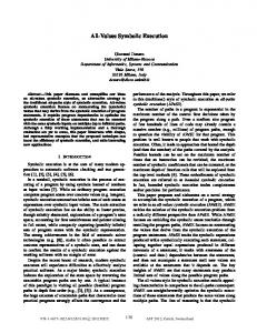
source Fig. 9. Grid topology containing 25 Contiki nodes. Each of the nodes can reach its first hop neighbors via broadcast. The solid arrows represent the preconfigured data path towards the sink node in the upper left corner, while the dashed gray arrows show the broadcast range of a transmission. In this particular scenario, there are six bystanders (gray shade) not involved in the communication. Test scenarios with 49 and 100 nodes look analogously.

IV. E VALUATION We implemented the algorithms in our tool KleeNet [6] which is the distributed version of the symbolic virtual machine KLEE [2]. KleeNet simulates a complete distributed system in a single process. It starts with k states representing the nodes in the network. As in any simulation, in each step KleeNet executes an event of a node and advances the time to the next event in the queue. If the symbolic execution of an event handler produces new states, they’re simply added to the state set. The state mapping algorithms are triggered either at the node’s local branch (COB) or upon a node’s message transmission (COW, SDS), respectively. Consequently, the newly created states (if any) are also added to the state set. For the evaluation, we use the latest Contiki OS [7] CVS snapshot, specifically the Rime communication stack [8]—a leightweight protocol stack designed for low-power radios. Note that KleeNet executes the software without any modifications prior testing. Thus, the evaluation results of SDE are also applicable to testing of similar distributed systems. A. Test setup The exemplary communication scenarios involve 25, 49, and 100 Contiki nodes, respectively. Each scenario is arranged in a linear grid topology (5x5, 7x7, and 10x10 nodes; cf. Figure 9). After network boot-up a node in the bottom right corner is configured to send a data packet every second to the sink node in the top left corner. Each packet of the transmitting node is perceived by its neighbors which in turn forward the data in a multi-hop fashion to the nodes towards the destination via a static route. The simulation time is 10 seconds. Without any symbolic input configured, KleeNet works as a simulator for one particular dscenario. Thus, we set-up KleeNet using a configuration file as follows: nodes on the data path towards the destination and their neighbors should symbolically drop one packet. One symbolic drop means that during reception of the first packet the receiving node’s state is forked by a network failure model. Then, in one state the radio receives the packet while in the other the packet is

State mapping algorithm Copy On Branch (COB) Copy On Write (COW) Super DStates (SDS)

Runtime 9h:39m (aborted) 1h:38m 19m

States

RAM

1,025,700 30,464 4,159

38.1 GB 3.4 GB 1.6 GB

TABLE I T EST RESULTS FOR THE 100 NODE SCENARIO WITH SYMBOLIC PACKET DROPS ENABLED .

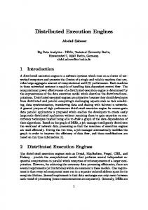
With growing network size, the performance gain of SDS grows as the number of bystanders increases. This validates the key idea of SDE—we can profit from the local nodes’ communication and thus avoid unnecessary state duplication which is extremely expensive in terms of execution time and memory consumption. C. Limitations and discussion

dropped. Further failures (packet duplicates, node failures and reboots) are implemented and configured in a similar fashion. Such symbolic failures help us to detect corner-cases before deployment which can lead to undefined or even erroneous distributed system behavior [6]. Each scenario was run in KleeNet using COB, COW, and the SDS algorithm, respectively. The tests were performed on a user-shared Intel Xeon 3.33GHz CPU machine with 64 GB of RAM. The memory cap per scenario was limited to approx. 40 GB of RAM to prevent swapping and other side-effects. For each run we sampled the execution time, the number of states, and the memory usage of the KleeNet process. B. Test results We summarized the results for the largest test scenario (100 nodes) in Table I to give an idea about the performance of the presented state mapping algorithms. Starting with COB, we had to abort the test after 9 hours of execution due to the physical memory limit of the shared machine. KleeNet generated 1.025.700 states so far which result in 10.257 unique dscenarios (100 states per dscenario). Upon each symbolic packet drop during the communication COB forked all its dstates’ states in the system, quickly exhausting the machine’s memory and slowing down KleeNet’s execution. Every duplicate state adds to the overall memory usage and is redundantly executed without discovering new code. In contrast to COB, COW performs significantly better resolving state conflicts only upon packet transmission. Therefore, COW forks its dstate’s states only when the sending state has at least one rival (cf. Section III). Nevertheless, each conflict resolution by COW creates duplicates, i.e., copies of bystanders which are not directly involved in the communication. Note that bystanders are not only the states which are not on the data path, but also states on the data path two or more hops away from the sending state. Finally, SDS eliminates all state conflicts without creating redundant duplicates of bystanders. The impact of duplicate reduction significantly speeds up KleeNet’s execution which is reflected in both, fast execution time and a low memory footprint. For a more detailed comparison over time we depicted the measurement results of all three scenarios in Figure 10. At the beginning of the execution, all graphs show a sudden state and memory consumption increase. In each run, KleeNet first loads the LLVM bytecode [9] containing nodes’ software which requires up to 1 GB of RAM in the 100 node scenario.

On the one hand, SDE scales well taking advantage of the nodes’ local communication, but on the other hand it is easy to set-up test scenarios or applications where COW and SDS algorithms perform nearly as bad as COB. One example would be a full-meshed network where nodes continuously transmit data to their k − 1 neighbors. Further examples comprise communication protocols based on network flooding such as neighbor discovery or data dissemination. Nonetheless, there are many distributed protocols and applications which would profit from SDE during testing. Another facet of SDE is the process of test case generation at the end of the symbolic execution. If someone wants to gather the test cases for all nodes in all dscenarios, the compact systems’ representation provided by the SDS algorithm has to be “exploded” to the output of COB to generate concrete test case values. The process of deliberate state explosion is very expensive in both execution time and memory but yet can be done incrementally, i.e., by forking states for a dscenario, generating test cases, and deleting the states could be done in one step. Nonetheless, the generation of all test cases at the end of execution is still by orders of magnitude faster than the execution using COB. V. R ELATED W ORK In this section we review the related work in the area of symbolic execution which comes closest to our work. From the vast number of symbolic execution approaches we only discuss those in more detail which consider the semantics of execution path order and their intra-dependencies. We implemented SDE in KleeNet [6] which is an extension to the symbolic virtual machine KLEE [2]. KLEE explores execution paths of single-threaded programs at high-coverage, but each of these paths is analyzed independently from all others. With KleeNet, we presented early ideas of SDE as an approach for 2–3 node scenarios and found subtle bugs in widely deployed sensornet software. In contrast to KleeNet, in this paper we generalize the ideas of SDE and detail on the state mapping algorithms and their efficacy independent from any specific implementation. Thus, the presented approach can be easily transferred to any other symbolic execution engine. Symbolic PathFinder [10] [11] (SPF) is a popular tool which combines symbolic execution, concrete execution, and model checking to generate test cases for Java programs. Being an extension to Java PathFinder [12], SPF employs its model checking capabilities such as thread interleaving testing and state backtracking. Consequently, the search is able to backtrack the execution states during exploration if, for example, a path condition becomes infeasible. In contrast, SDE

104 103 102

104

102 0 10

105

(a) 25 nodes scenario: state growth over time.

105

104 103

104

104

103

102 0 10

105

(c) 49 nodes scenario: state growth over time.

104

memory [MB] (log scale)

105

102 101 100 0 10

101

102 103 time [s] (log scale)

COW finished

103

SDS finished

number of states (log scale)

106

105

COB COW SDS

104

(e) 100 nodes scenario: state growth over time.

101

104

102 103 time [s] (log scale)

105

(d) 49 nodes scenario: memory growth over time.

States

COB aborted

107

COB COW SDS

105

RAM

COB COW SDS

COB aborted

102 103 time [s] (log scale)

RAM

104

103

102 0 10

101

102 103 time [s] (log scale)

COW finished

101

COB finished

100 0 10

COW finished

102 101

105

COB finished

COB COW SDS

SDS finished

number of states (log scale)

105

104

102 103 time [s] (log scale)

(b) 25 nodes scenario: memory growth over time.

States

memory [MB] (log scale)

106

101

SDS finished

102 103 time [s] (log scale)

103

COW finished

101

104

SDS finished

100 0 10

COB finished

101

COB COW SDS

COB finished

COB COW SDS

RAM SDS finished COW finished

105

SDS finished COW finished

number of states (log scale)

105

States

memory [MB] (log scale)

106

104

105

(f) 100 nodes scenario: memory growth over time.

Fig. 10. Test results for 25, 49, and 100 node scenarios. Each scenario was run three times using COB, COW, and SDS algorithm, respectively. For the 100 node scenario, we aborted KleeNet’s execution using COB since the memory consumption was getting close to the actual physical machine’s limits.

targets a compact representation of the symbolic system state where execution states could be shared among several SPF “runs”. Moreover, SDE does not support state backtracking. Model-based testing of interleaved processes using symbolic execution is introduced in [13]. The authors employ an executable modeling language to capture distribution, concurrency, and asynchronous communication. The system performs a concrete and a symbolic run in parallel gradually constructing path constraints for a distributed application. The small case studies of the semi-automated tool are promising, however, the authors don’t address state conflicts and how they’re resolved between the test runs. Execution Synthesis [3] (ESD) is a further technique to automatically generate deterministic thread schedules and concrete inputs guiding multi-threaded programs to known bug symptoms. Starting with a bug report and a program, ESD first performs static analysis to derive the search space towards the goal described in the report. Second, it employs symbolic execution using KLEE to narrow down the over-approximated outcome of static analysis to one feasible execution path. Third, ESD treats the thread scheduler to be symbolic in order to explore different serialized execution paths of a multithreaded program. The decision to preempt or not to preempt a thread is very similar to the network/node failures used in KleeNet. Finally, one of the thread schedules hits the bug which can be replayed and analyzed by the developers. From the modeling point of view, threads in ESD can be seen as nodes in SDE. In contrast to ESD, however, SDE eliminates the execution of redundant paths which have the same semantics within different execution scenarios, i.e., thread schedules. Thus, ESD might profit from the SDE’s approach to reduce the execution time and memory footprint during the search. Recently, a number of concolic approaches [14] [15] [16] were proposed combining both concrete and symbolic execution within different execution environments. However, these only consider a single instance of software under test and not a distributed execution. In contrast, SDE is applied to distributed systems capturing asynchronous communication over the network. Noteworthy, SDE doesn’t model message interleaving which would lead to additional state growth. VI. C ONCLUSION We presented SDE—an approach enabling scalable symbolic execution of distributed systems. We developed a state mapping algorithm which performs efficiently in distributed systems profiting from the nodes’ local communication. We demonstrated the merits of SDE by evaluating a Contiki-based sensornet in KleeNet. Finally, we discussed SDE’s limitations and identified its potential in related application areas. In the future, we plan to parallelize SDE’s implementation in KleeNet to speed up testing on multicore machines. For the parallelization, we have to identify the sets of states which can be safely offloaded on other cores and thus can be independently executed. Furthermore, we aim to implement

incremental test case generation which is important for largescale test scenarios. Overall, we see SDE as a general idea for symbolic execution of distributed systems which can be utilized in other tools and frameworks. This would leverage the existing power of symbolic execution to even more rigorous software testing. ACKNOWLEDGMENTS We thank Christopher Gill, our shepherd, and Florian Schmidt for their help in improving our paper. We are grateful ´ to J´o Agila Bitsch Link for his contribution with the automatic generation of evaluation figures. This work is partly supported by DFG UMIC research cluster of RWTH Aachen University. R EFERENCES [1] J. C. King, “Symbolic Execution and Program Testing,” Communications of the ACM, vol. 19, no. 7, pp. 385–394, 1976. [2] C. Cadar, D. Dunbar, and D. Engler, “KLEE: Unassisted and Automatic Generation of High-Coverage Tests for Complex Systems Programs,” in USENIX Symposium on Operating Systems Design and Implementation, 2008. [3] C. Zamfir and G. Candea, “Execution Synthesis: A Technique for Automated Software Debugging,” in Proceedings of the 5th ACM SIGOPS/EuroSys European Conference on Computer Systems (EuroSys), Paris, France, 2010. [Online]. Available: http://dslab.epfl.ch/pubs/esd [4] V. Chipounov and G. Candea, “Reverse Engineering of Binary Device Drivers with RevNIC,” in Proceedings of the 5th ACM SIGOPS/EuroSys European Conference on Computer Systems (EuroSys), Paris France, April 2010, Paris, France, 2010. [5] C. S. Pˇasˇareanu, P. C. Mehlitz, D. H. Bushnell, K. Gundy-Burlet, M. Lowry, S. Person, and M. Pape, “Combining Unit-level Symbolic Execution and System-level Concrete Execution for Testing NASA Software,” in Proceedings of the 2008 International Symposium on Software Testing and Analysis, ser. ISSTA ’08. ACM, 2008. [6] R. Sasnauskas, O. Landsiedel, H. Alizai, C. Weise, S. Kowalewski, and K. Wehrle, “KleeNet: Discovering Insidious Interaction Bugs in Wireless Sensor Networks Before Deployment,” in International Conference on Information Processing in Sensor Networks (ACM IPSN/SPOTS). New York, NY, USA: ACM, 2010, pp. 186–196. [7] A. Dunkels, B. Gronvall, and T. Voigt, “Contiki - A Lightweight and Flexible Operating System for Tiny Networked Sensors,” in LCN, 2004. ¨ [8] A. Dunkels, F. Osterlind, and Z. He, “An Adaptive Communication Architecture for Wireless Sensor Networks,” in Proceedings of the Fifth ACM Conference on Networked Embedded Sensor Systems (SenSys 2007), Sydney, Australia, Nov. 2007. [9] C. Lattner and V. Adve, “LLVM: A Compilation Framework for Lifelong Program Analysis & Transformation,” in CGO ’04: Proc. of the international symposium on Code generation and optimization, 2004. [10] C. S. P˘as˘areanu and N. Rungta, “Symbolic PathFinder: Symbolic Execution of Java Bytecode,” in Proceedings of the IEEE/ACM International Conference on Automated Software Engineering, ser. ASE ’10. New York, NY, USA: ACM, 2010, pp. 179–180. [11] S. Anand, C. S. Pasareanu, and W. Visser, “JPF-SE: A Symbolic Execution Extension to Java Pathfinder,” in TACAS, 2007. [12] W. Visser, K. Havelund, G. Brat, and S. Park, “Model Checking Programs,” in Proceedings of the 15th IEEE International Conference on Automated Software Engineering, ser. ASE ’00. Washington, DC, USA: IEEE Computer Society, 2000, pp. 3–. [13] A. Griesmayer, B. Aichernig, E. B. Johnsen, and R. Schlatte, “Dynamic symbolic execution for testing distributed objects,” in Proceedings of the 3rd International Conference on Tests and Proofs, ser. TAP ’09. Berlin, Heidelberg: Springer-Verlag, 2009, pp. 105–120. [Online]. Available: http://dx.doi.org/10.1007/978-3-642-02949-3 9 [14] R. Majumdar and K. Sen, “Hybrid Concolic Testing,” in ICSE, 2007. [15] K. Sen, D. Marinov, and G. Agha, “CUTE: A Concolic Unit Testing Engine for C,” in ESEC/FSE-13, 2005. [16] V. Chipounov, V. Kuznetsov, and G. Candea, “S2E: A Platform for InVivo Multi-Path Analysis of Software Systems,” in Proceedings of the 16th International Conference on Architectural Support for Programming Languages and Operating Systems, 2011.