Scaling Limits for Internal Aggregation Models with Multiple Sources

arXiv:0712.3378v2 [math.PR] 2 May 2009

Scaling Limits for Internal Aggregation Models with Multiple Sources Lionel Levine∗ and Yuval Peres† University of California, Berkeley and Microsoft Research May 1, 2009

Abstract We study the scaling limits of three different aggregation models on Zd : internal DLA, in which particles perform random walks until reaching an unoccupied site; the rotor-router model, in which particles perform deterministic analogues of random walks; and the divisible sandpile, in which each site distributes its excess mass equally among its neighbors. As the lattice spacing tends to zero, all three models are found to have the same scaling limit, which we describe as the solution to a certain PDE free boundary problem in Rd . In particular, internal DLA has a deterministic scaling limit. We find that the scaling limits are quadrature domains, which have arisen independently in many fields such as potential theory and fluid dynamics. Our results apply both to the case of multiple point sources and to the DiaconisFulton smash sum of domains. ∗

supported by an NSF Graduate Research Fellowship, and NSF grant DMS-0605166 partially supported by NSF grant DMS-0605166 Key words: asymptotic shape, divisible sandpile, Green’s function, Hele-Shaw flow, internal diffusion limited aggregation, obstacle problem, quadrature domain, rotor-router model 2000 Mathematics Subject Classifications: Primary 60G50; Secondary 35R35, 31C20 †

1

Contents 1 Introduction

2

2 Potential Theory Background 2.1 Least Superharmonic Majorant . . . . . . . . . . . 2.2 Superharmonic Potentials . . . . . . . . . . . . . . 2.3 Boundary Regularity for the Obstacle Problem . . 2.4 Convergence of Obstacles, Majorants and Domains 2.5 Discrete Potential Theory . . . . . . . . . . . . . .

. . . . .

. . . . .

. . . . .

. . . . .

. . . . .

. . . . .

11 12 13 15 17 19

3 Divisible Sandpile 22 3.1 Abelian Property and Least Action Principle . . . . . . . . . 22 3.2 Convergence of Odometers . . . . . . . . . . . . . . . . . . . . 24 3.3 Convergence of Domains . . . . . . . . . . . . . . . . . . . . . 29 4 Rotor-Router Model 31 4.1 Convergence of Odometers . . . . . . . . . . . . . . . . . . . . 32 4.2 Convergence of Domains . . . . . . . . . . . . . . . . . . . . . 37 5 Internal DLA 41 5.1 Inner Estimate . . . . . . . . . . . . . . . . . . . . . . . . . . 41 5.2 Outer Estimate . . . . . . . . . . . . . . . . . . . . . . . . . . 49 6 Multiple Point Sources 53 6.1 Associativity and Continuity of the Smash Sum . . . . . . . . 54 6.2 Smash Sums of Balls . . . . . . . . . . . . . . . . . . . . . . . 57 7 Potential Theory Proofs 7.1 Least Superharmonic Majorant . . . 7.2 Boundary Regularity . . . . . . . . . 7.3 Convergence of Obstacles, Majorants 7.4 Discrete Potential Theory . . . . . . 8 Open Problems

1

. . . . . . . . . . . . . . . . and Domains . . . . . . . .

. . . .

. . . .

. . . .

. . . .

. . . .

. . . .

60 60 63 68 69 71

Introduction

Given finite sets A, B ⊂ Zd , Diaconis and Fulton [7] defined the smash sum A ⊕ B as a certain random set whose cardinality is the sum of the

2

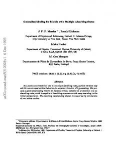
Figure 1: Smash sum of two squares overlapping in a smaller square, for internal DLA (top left), the rotor-router model (top right), and the divisible sandpile. cardinalities of A and B. Write A ∩ B = {x1 , . . . , xk }. To construct the smash sum, begin with the union C0 = A ∪ B and for each j = 1, . . . , k let Cj = Cj−1 ∪ {yj } where yj is the endpoint of a simple random walk started at xj and stopped on exiting Cj−1 . Then define A ⊕ B = Ck . The key observation of [7] is that the law of A ⊕ B does not depend on the ordering of the points xj . The sum of two squares in Z2 overlapping in a smaller square is pictured in Figure 1. In Theorem 1.3, below, we prove that as the lattice spacing goes to zero, the smash sum A ⊕ B has a deterministic scaling limit in Rd . Before stating 3

our main results, we describe some related models and discuss our technique for identifying their common scaling limit, which comes from the theory of free boundary problems in PDE. The Diaconis-Fulton smash sum generalizes the model of internal diffusion limited aggregation (“internal DLA”) studied in [20], and in fact was part of the original motivation for that paper. In classical internal DLA, we start with n particles at the origin o ∈ Zd and let each perform simple random walk until it reaches an unoccupied site. The resulting random set of n occupied sites in Zd can be described as the n-fold smash sum of {o} with itself. We will use the term internal DLA to refer to the same process run from an arbitrary starting configuration of particles. In this broader sense of the term, both the Diaconis-Fulton sum and the model studied in [20] are particular cases of internal DLA. In defining the smash sum A ⊕ B, various alternatives to random walk are possible. Rotor-router walk is a deterministic analogue of random walk, first studied by Priezzhev et al. [24] under the name “Eulerian walkers.” At each site in Z2 is a rotor pointing north, south, east or west. A particle performs a nearest-neighbor walk on the lattice according to the following rule: during each time step, the rotor at the particle’s current location is rotated clockwise by 90 degrees, and the particle takes a step in the direction of the newly rotated rotor. In higher dimensions, the model can be defined analogously by repeatedly cycling the rotors through an ordering of the 2d cardinal directions in Zd . The sum of two squares in Z2 using rotor-router walk is pictured in Figure 1; all rotors began pointing west. The shading in the figure indicates the final rotor directions, with four different shades corresponding to the four possible directions. The divisible sandpile model uses continuous amounts of mass in place of discrete particles. A lattice site is full if it has mass at least 1. Any full site can topple by keeping mass 1 for itself and distributing the excess mass equally among its neighbors. At each time step, we choose a full site and topple it. As time goes to infinity, provided each full site is eventually toppled, the mass approaches a limiting distribution in which each site has mass ≤ 1; this is proved in [21]. Note that individual topplings do not commute. However, the divisible sandpile is “abelian” in the sense that any sequence of topplings produces the same limiting mass distribution; this is proved in Lemma 3.1. Figure 1 shows the limiting domain of occupied sites resulting from starting mass 1 on each of two squares in Z2 , and mass 2 on the smaller square where they intersect. Figure 1 raises a few natural questions: as the underlying lattice spacing becomes finer and finer, will the smash sum A ⊕ B tend to some limiting 4

shape in Rd , and if so, what is this shape? Will it be the same limiting shape for all three models? To see how we might identify the limiting shape, consider the divisible sandpile odometer function u(x) = total mass emitted from x. Since each neighbor y ∼ x emits an equal amount of mass to each of its 2d 1 P neighbors, the total mass received by x from its neighbors is 2d y∼x u(y), hence ∆u(x) = ν(x) − σ(x) (1) where σ(x) and ν(x) are the initial and final amounts of mass at x, respectively. Here ∆ is the discrete Laplacian in Zd , defined by ∆u(x) = 1 P y∼x u(y) − u(x). 2d Equation (1) suggests the following approach to finding the limiting shape. We first construct a function on Zd whose Laplacian is σ − 1; an example is the function X g1 (x, y)σ(y) (2) γ(x) = −|x|2 − y∈Zd

where in dimension d ≥ 3 the Green’s function g1 (x, y) is the expected number of times a simple random walk started at x visits y (in dimension d = 2 we use the recurrent potential kernel in place of the Green’s function). The sum u+γ is then a superharmonic function on Zd ; that is, ∆(u+γ) ≤ 0. Moreover if f ≥ γ is any superharmonic function lying above γ, then f −γ−u is superharmonic on the domain D = {x ∈ Zd |ν(x) = 1} of fully occupied sites, and nonnegative outside D, hence nonnegative everywhere. Thus we have proved the following lemma of [21]. Lemma 1.1. Let σ be a nonnegative function on Zd with finite support. Then the odometer function for the divisible sandpile started with mass σ(x) at each site x is given by u=s−γ where γ is given by (2), and s(x) = inf{f (x)|f is superharmonic on Zd and f ≥ γ} is the least superharmonic majorant of γ. For a reformulation of this lemma as a “least action principle,” see Lemma 3.2. 5

Figure 2: The obstacles γ corresponding to starting mass 1 on each of two overlapping disks (top) and mass 100 on each of two nonoverlapping disks. Lemma 1.1 allows us to formulate the problem in a way which translates naturally to the continuum. Given a function σ on Rd representing the initial mass density, by analogy with (2) we define the obstacle Z 2 γ(x) = −|x| − g(x, y)σ(y)dy Rd

where g(x, y) is the harmonic potential on Rd proportional to |x − y|2−d in dimensions d ≥ 3 and to − log |x − y| in dimension two. We then let s(x) = inf{f (x)|f is continuous, superharmonic and f ≥ γ}. The odometer function for σ is then given by u = s−γ, and the final domain of occupied sites is given by D = {x ∈ Rd |s(x) > γ(x)}.

(3)

This domain D is called the noncoincidence set for the obstacle problem with obstacle γ; for an in-depth discussion of the obstacle problem, see [10]. If A, B are bounded open sets in Rd , we define the smash sum of A and B as A⊕B =A∪B∪D (4) 6

where D is given by (3) with σ = 1A + 1B . In the two-dimensional setting, an alternative definition of the smash sum in terms of quadrature identities is mentioned in [14]. By analogy with the discrete case, we would expect that L(A ⊕ B) = L(A) + L(B), where L denotes Lebesgue measure in Rd . This is proved in Corollary 2.13. More generally, if h is a superharmonic function on Zd , and σ is a mass d configuration P for the divisible sandpile (so each site x ∈ Z has mass σ(x)), the sum x∈Zd h(x)σ(x) can only decrease when we perform a toppling. Thus X X h(x)ν(x) ≤ h(x)σ(x), (5) x∈Zd

x∈Zd

where ν is the final mass configuration. We therefore expect the domain D given by (3) to satisfy the quadrature inequality Z Z h(x)dx ≤ h(x)σ(x)dx (6) D

D

for all integrable superharmonic functions h on D. For a proof under suitable smoothness assumptions on σ and h, see Proposition 2.11; see also [27]. A domain D ⊂ Rd satisfying an inequality of the form (6) is called a quadrature domain for σ. Such domains are widely studied in potential theory and have a variety of applications in fluid dynamics [6, 25]. For more on quadrature domains and their connection with the obstacle problem, see [1, 5, 16, 18, 27, 28]. Equation (5) can be regarded as a discrete analogue of a quadrature inequality; in this sense, the three aggregation models studied in this paper produce discrete analogues of quadrature domains. Indeed, these aggregation models can be interpreted as discrete analogues of Hele-Shaw flow [6, 31], which produces quadrature domains in the continuum. The main goal of this paper is to prove that if any of our three aggregation models – internal DLA, rotor-router, or divisible sandpile – is run on finer and finer lattices with initial mass densities converging in an appropriate sense to σ, the resulting domains of occupied sites will converge in an appropriate sense to the domain D given by (3). In order to state our main result, let us define the appropriate notion of convergence of domains, which amounts essentially to convergence in the Hausdorff metric. Fix a sequence δn ↓ 0 representing the lattice spacing. Given domains An ⊂ δn Zd and D ⊂ Rd , write An → D if for any > 0 D ∩ δn Zd ⊂ An ⊂ D 7

(7)

for all sufficiently large n. Here D and D denote respectively the inner and outer -neighborhoods of D: D = {x ∈ D | B(x, ) ⊂ D} D = {x ∈ Rd | B(x, ) 6⊂ Dc }

(8)

where B(x, ) is the ball of radius centered at x. d For x ∈ δn Zd we write x = x + δ2n , x − δ2n . For t ∈ R write bte for the closest integer to t, rounding up if t ∈ Z + 21 . The initial data for each of our lattice models consists of a function σn : δn Zd → Z≥0 representing the number of particles (or amount of mass) at each lattice site; we think of σn as a density with respect to counting measure on δn Zd , and refer to it as the “initial density.” Throughout this paper, to avoid trivialities we work in dimension d ≥ 2. Our main result is the following. Theorem 1.2. Let Ω ⊂ Rd , d ≥ 2 be a bounded open set, and let σ : Rd → Z≥0 be a bounded function which is continuous almost everywhere, satisfying ¯ Let Dn , Rn , In be the domains of occupied sites formed from {σ ≥ 1} = Ω. the divisible sandpile, rotor-router model, and internal DLA, respectively, in the lattice δn Zd started from initial density Z −d σn (x) = δn σ(y)dy . x

Then as n ↑ ∞ Dn , Rn → D ∪ Ω; and if δn log n ↓ 0, then with probability one In → D ∪ Ω where D is given by (3), and the convergence is in the sense of (7). Remark. When forming the rotor-router domains Rn , the initial rotors in each lattice δn Zd may be chosen arbitrarily. As an immediate consequence, all three lattice models have a rotationallyinvariant scaling limit. This follows from the rotational symmetry of the obstacle problem: if ρ is a rotation of Rd , and D is the noncoincidence set (3) for initial density σ, then the noncoincidence set for initial density σ ◦ρ−1 is ρD.

8

We prove a somewhat more general form of Theorem 1.2 which allows for some flexibility in how the discrete density σn is constructed from σ. In particular, taking σ = 1A¯ + 1B¯ we obtain the following theorem, which explains the similarity of the three smash sums pictured in Figure 1. Theorem 1.3. Let A, B ⊂ Rd be bounded open sets whose boundaries have measure zero. Let Dn , Rn , In be the smash sum of A ∩ δn Zd and B ∩ δn Zd , formed using divisible sandpile, rotor-router and internal DLA dynamics, respectively. Then as n ↑ ∞ Dn , Rn → A ⊕ B; and if δn log n ↓ 0, then with probability one In → A ⊕ B where A ⊕ B is given by (4), and the convergence is in the sense of (7). For the divisible sandpile, Theorem 1.2 can be generalized by dropping the requirement that σ be integer valued; see Theorem 3.9 for the precise statement. Taking σ real-valued is more problematic in the case of the rotor-router model and internal DLA, since these models work with discrete particles. Still, one might wonder if, for example, given a domain A ⊂ Rd , starting each even site in A ∩ δn Zd with one particle and each odd site with two particles, the resulting domains Rn , In would converge to the noncoincidence set D for density σ = 23 1A . This is in fact the case: if σn is a density on δn Zd , as long as a certain “smoothing” of σn converges to σ, the rotor-router and internal DLA domains started from initial density σn will converge to D. See Theorems 4.8 and 5.1 for the precise statements. One interesting case not covered by Theorems 1.2 and 1.3 is the case of multiple point sources. Lawler, Bramson and Griffeath [20] showed that the scaling limit of internal DLA in Zd with a single point source of particles is a Euclidean ball. In [21], the present authors showed that for rotor-router aggregation and the divisible sandpile in Zd with a single point source, the scaling limit in both cases is also a Euclidean ball. For x ∈ Rd write x:: for the closest lattice point in δn Zd , breaking ties to the right. Our shape theorem for multiple point sources, which is deduced from Theorem 1.3 using the main results of [20] and [21], is the following. Theorem 1.4. Fix x1 , . . . , xk ∈ Rd and λ1 , . . . , λk > 0. Let Bi be the ball of volume λi centered at xi . Fix a sequence δn ↓ 0, and for x ∈ δn Zd let $ % k X −d σn (x) = δn λi 1{x=x::i } . i=1

9

Figure 3: The rotor-router model in Z2 started from two point sources on the x-axis. The boundary of the limiting shape is an algebraic curve (11) of degree 4. Let Dn , Rn , In be the domains of occupied sites in δn Zd formed from the divisible sandpile, rotor-router model, and internal DLA, respectively, started from initial density σn . Then as n → ∞ Dn , Rn → B1 ⊕ . . . ⊕ Bk ;

(9)

and if δn ≤ 1/n, then with probability one In → B1 ⊕ . . . ⊕ Bk where ⊕ denotes the smash sum (4), and the convergence is in the sense of (7). Implicit in (9) is the associativity of the smash sum operation, which is not readily apparent from the definition (4). For a proof of associativity, see Lemma 6.1. Alternatively, the associativity follows from basic properties of “partial balayage” operators on measures on Rd ; see [15, Theorem 2.2(iii)]. For related results in dimension two, see [26, Prop. 3.10] and [31, section 2.4]. We remark that a similar model of internal DLA with multiple point sources was studied by Gravner and Quastel [12], who also obtained a variational solution. In their model, instead of starting with a fixed number of 10

particles, each source xi emits particles according to a Poisson process. The shape theorems of [12] concern convergence in the sense of volume, which is a weaker form of convergence than that studied in the present paper. In Proposition 6.6, we show that the smash sum of balls B1 ⊕ . . . ⊕ Bk arising in Theorem 1.4 obeys the classical quadrature inequality Z h(x)dx ≤ B1 ⊕...⊕Bk

k X

λi h(xi )

(10)

i=1

for all integrable superharmonic functions h on B1 ⊕ . . . ⊕ Bk , with equality if h is harmonic. This can be regarded as a generalization of the classical mean value property of harmonic functions, which corresponds to the case k = 1. Let B1 , . . . , Bk be disks in R2 with distinct centers x1 , . . . , xk . From (10) and work of Aharonov and Shapiro [1] and Gustafsson [13, 14] it follows that that the boundary ∂(B1 ⊕ . . . ⊕ Bk ) lies on an algebraic curve of degree 2k. More precisely, there is a polynomial P ∈ R[x, y] of the form P (x, y) = x2 + y 2

k

+ lower order terms

and there is a finite set of points E ⊂ R2 , possibly empty, such that ∂(B1 ⊕ . . . ⊕ Bk ) = {(x, y) ∈ R2 |P (x, y) = 0} − E. For example, if B1 and B2 are disks of equal radius r > 1 centered at (1, 0) and (−1, 0), then ∂(B1 ⊕ B2 ) is given by the quartic curve [29] x2 + y 2

2

− 2r2 x2 + y 2 − 2(x2 − y 2 ) = 0.

(11)

This curve describes the shape of the rotor-router model with two point sources pictured in Figure 3.

2

Potential Theory Background

In this section we review the basic properties of superharmonic potentials and of the least superharmonic majorant. The proofs are deferred to section 7. In view of the diverse readership who might be interested in the models we study, we have elected to include somewhat more than the usual amount of background material.

11

2.1

Least Superharmonic Majorant

Since we will often be working with functions on Rd which may not be twice differentiable, it is desirable to define superharmonicity without making reference to the Laplacian. Instead we use the mean value property. A function u on an open set Ω ⊂ Rd is superharmonic if it is lower-semicontinuous and for any ball B(x, r) ⊂ Ω Z 1 u(x) ≥ Ar u(x) := u(y)dy. (12) ωd rd B(x,r) Here ωd is the volume of the unit ball in Rd . We say that u is subharmonic if −u is superharmonic, and harmonic if it is both super- and subharmonic. The following properties of superharmonic functions are well known; for proofs, see e.g. [3], [8] or [22]. Lemma 2.1. Let u be a superharmonic function on an open set Ω ⊂ Rd ¯ Then extending continuously to Ω. ¯ on the boundary. (i) u attains its minimum in Ω ¯ harmonic on Ω, and h = u on ∂Ω, then u ≥ h. (ii) If h is continuous on Ω, (iii) If B(x, r0 ) ⊂ B(x, r1 ) ⊂ Ω, then Ar0 u(x) ≥ Ar1 u(x). (iv) If u is twice differentiable on Ω, then ∆u ≤ 0 on Ω. (v) If B ⊂ Ω is an open ball, and v is a function on Ω which is har¯ and agrees with u on B c , then v is monic on B, continuous on B, superharmonic. Given a function γ on Rd which is bounded above, the least superharmonic majorant of γ (also called the solution to the obstacle problem with obstacle γ) is the function s(x) = inf{f (x)|f is continuous, superharmonic and f ≥ γ}.

(13)

Note that since γ is bounded above, the infimum is taken over a nonempty set. Lemma 2.2. Let γ be a uniformly continuous function which is bounded above, and let s be given by (13). Then 12

(i) s is superharmonic. (ii) s is continuous. (iii) s is harmonic on the domain D = {x ∈ Rd |s(x) > γ(x)}.

2.2

Superharmonic Potentials

Next we describe the particular class of obstacles which relate to the aggregation models we are studying. For a bounded measurable function σ on Rd with compact support, write Z Gσ(x) = g(x, y)σ(y)dy, (14) Rd

where

Here ad =

( − π2 log |x − y|, d = 2; g(x, y) = ad |x − y|2−d , d ≥ 3. 2 (d−2)ωd ,

(15)

where ωd is the volume of the unit ball in Rd . Note that

(15) differs by a factor of 2d from the standard harmonic potential in Rd ; however, the normalization we have chosen is most convenient when working with the discrete Laplacian and random walk. The following result is standard; see [8, Theorem 1.I.7.2]. Lemma 2.3. Let σ be a measurable function on Rd with compact support. (i) If σ is bounded, then Gσ is continuous. (ii) If σ is C 1 , then Gσ is C 2 and ∆Gσ = −2dσ.

(16)

Regarding (ii), if we remove the smoothness assumption on σ, equation (16) remains true in the sense of distributions. For our applications, however, we will not need this, and the following lemma will suffice. Lemma 2.4. Let σ be a bounded measurable function on Rd with compact support. If σ ≥ 0 on an open set Ω ⊂ Rd , then Gσ is superharmonic on Ω.

13

By applying Lemma 2.4 both to σ and to −σ, we obtain that Gσ is harmonic off the support of σ. Let B = B(o, r) be the ball of radius r centered at the origin in Rd . We compute in dimensions d ≥ 3  2  dr − |x|2 , |x| < r d−2 G1B (x) = 2r2 r d−2 (17)  , |x| ≥ r. d−2 |x| Likewise in two dimensions ( r2 (1 − 2 log r) − |x|2 , |x| < r G1B (x) = −2r2 log |x|, |x| ≥ r.

(18)

Fix a bounded nonnegative function σ on Rd with compact support, and let γ(x) = −|x|2 − Gσ(x).

(19)

Let s(x) = inf{f (x)|f is continuous, superharmonic and f ≥ γ}

(20)

be the least superharmonic majorant of γ, and let D = {x ∈ Rd |s(x) > γ(x)}

(21)

be the noncoincidence set. Lemma 2.5.

(i) γ(x) + |x|2 is subharmonic on Rd .

(ii) If σ ≤ M on an open set Ω ⊂ Rd , then γ(x) − (M − 1)|x|2 is superharmonic on Ω. Lemma 2.6. Let u = s − γ, where γ and s are given by (19) and (20). Then (i) u(x) − |x|2 is superharmonic on Rd . (ii) If σ ≤ M on an open set Ω ⊂ Rd , then u(x) + M |x|2 is subharmonic on Ω. Lemma 2.7. Let D be given by (21). Then {σ > 1}o ⊂ D. The next lemma concerns the monotonicity of our model: by starting with more mass, we obtain a larger odometer and a larger noncoincidence set; see also [27, Lemma 7.1]. 14

Lemma 2.8.R Let σ1 ≤ σ2 be functions on Rd with compact support, and suppose that Rd σ2 (x)dx < ∞. Let γi (x) = −|x|2 − Gσi (x),

i = 1, 2.

Let si be the least superharmonic majorant of γi , let ui = si − γi , and let Di = {x|si (x) > γi (x)}. Then u1 ≤ u2 and D1 ⊂ D2 . Our next lemma shows that we can restrict to a domain Ω ⊂ Rd when taking the least superharmonic majorant, provided that Ω contains the noncoincidence set. Lemma 2.9. Let γ, s, D be given by (19)-(21). Let Ω ⊂ Rd be an open set with D ⊂ Ω. Then s(x) = inf{f (x)|f is superharmonic on Ω, continuous, and f ≥ γ}. (22)

2.3

Boundary Regularity for the Obstacle Problem

Next we turn to the regularity of the solution to the obstacle problem (20) and of the free boundary ∂D. There is a substantial literature on boundary regularity for the obstacle problem. In our setting, however, extra care must be taken near points where σ(x) = 1: at these points the obstacle (19) is harmonic, and the free boundary can be badly behaved. One approach, adopted in [17], is to reformulate the obstacle problem in Rd as an obstacle problem on the set {σ > 1}. The results of [17] apply in the situation that σ ≥ 1 everywhere, but we will want to relax this condition. We show only the minimal amount of regularity required for the proofs of our main theorems. Much stronger regularity results are known in related settings; see, for example, [4, 5]. The following lemma shows that if the obstacle is sufficiently smooth, then the superharmonic majorant cannot separate too quickly from the obstacle near the boundary of the noncoincidence set. As usual, we write D = {x ∈ D | B(x, ) ⊂ D}

(23)

for the inner -neighborhood of D. Lemma 2.10. Let σ be a C 1 function on Rd with compact support. Let γ, s, D be given by (19)-(21), and write u = s − γ. Then u is C 1 , and for y ∈ ∂D we have |∇u(y)| ≤ C0 , for a constant C0 depending on σ. 15

Next we showR that mass is conserved in our model: the amount of mass starting in D is D σ(x)dx, while the amount of mass ending in D is L(D), the Lebesgue measure of D. Since no mass moves outside of D, we expect these two quantities to be equal. Although this seems intuitively obvious, the proof takes some work because we have no a priori control of the domain D. In particular, we first need to show that the boundary of D cannot have positive d-dimensional Lebesgue measure. Proposition 2.11. Let σ be a C 1 function on Rd with compact support, such that L(σ −1 (1)) = 0. Let D be given by (21). Then (i) L(∂D) = 0. ¯ which is superharmonic on D, (ii) For any function h ∈ C 1 (D) Z Z h(x)dx ≤ h(x)σ(x)dx. D

D

Note that by applying (ii) both to h and to −h, equality holds whenever h is harmonic on D. In particular, taking h ≡ 1 yields the conservation of R mass: D σ(x)dx = L(D). We will also need a version of Proposition 2.11 which does not assume that σ is C 1 or even continuous. We can replace the C 1 assumption and the condition that L(σ −1 (1)) = 0 by the following condition. For all x ∈ Rd either σ(x) ≤ λ or σ(x) ≥ 1

(24)

for a constant λ < 1. Then we have the following result. Proposition 2.12. Let σ be a bounded function on Rd with compact support. e = D ∪ {σ ≥ 1}o . If σ is continuous almost Let D be given by (21), and let D everywhere and satisfies (24), then e = 0. (i) L ∂ D R (ii) L D = D σ(x)dx. R e = e σ(x)dx. (iii) L D D In particular, taking σ = 1A + 1B , we have e A⊕B =A∪B∪D =D where ⊕ denotes the smash sum (4). From (iii) we obtain the volume additivity of the smash sum. 16

Corollary 2.13. Let A, B ⊂ Rd be bounded open sets whose boundaries have measure zero. Then L(A ⊕ B) = L(A) + L(B). Our next lemma describes the domain resulting from an initial mass density m > 1 on a ball in Rd . Not surprisingly, the result is another ball, concentric with the original, of m times the volume. In particular, if m is an integer, the m-fold smash sum of a ball with itself is again a ball. Lemma 2.14. Fix m > 1, and let D be given by (21) with σ = m1B(o,r) . Then D = B(o, m1/d r). Proof. Since γ(x) = −|x|2 − Gσ(x) is spherically symmetric and the least superharmonic majorant commutes with rotations, D is a ball centered at the origin. By Proposition 2.12(ii) we have L(D) = mL(B(o, r)). Next we show that the noncoincidence set is bounded; see also [27, Lemma 7.2]. Lemma 2.15. Let σ be a function on Rd with compact support, satisfying 0 ≤ σ ≤ M . Let D be given by (21). Then D is bounded. Proof. Let B = B(o, r) be a ball containing the support of σ. By Lemmas 2.8 and 2.14, the difference s − γ is supported in B(o, M 1/d r).

2.4

Convergence of Obstacles, Majorants and Domains

In broad outline, many of our arguments have the following basic structure: convergence of densities =⇒ convergence of obstacles =⇒ convergence of majorants =⇒ convergence of domains. An appropriate convergence of starting densities is built into the hypotheses of the theorems. From these hypotheses we use Green’s function estimates to deduce the relevant convergence of obstacles. Next, properties of the obstacle can often be parlayed into corresponding properties of the least superharmonic majorant. Finally, deducing convergence of domains (i.e., noncoincidence sets) from the convergence of the majorants often requires additional regularity assumptions. The following lemma illustrates this basic three-step approach. 17

Lemma 2.16. Let σ and σn , n = 1, 2, . . . be densities on Rd satisfying 0 ≤ σ, σn ≤ M 1B for a constant M and ball B = B(o, R). If σn → σ in L1 , then (i) Gσn → Gσ uniformly on compact subsets of Rd . (ii) sn → s uniformly on compact subsets of Rd , where s, sn are the least superharmonic majorants of the functions γ = −|x|2 − Gσ, and γn = −|x|2 − Gσn , respectively. (iii) For any > 0 we have D ⊂ D(n) for all sufficiently large n, where D, D(n) are the noncoincidence sets {s > γ} and {sn > γn }, respectively. According to the following lemma, a nonnegative function on Zd with bounded Laplacian can grow at most quadratically. Lemma 2.17. Fix 0 < β < 1. There is a constant cβ such that any nonnegative function f on Zd with f (o) = 0 and |∆f | ≤ λ in B(o, R) satisfies f (x) ≤ cβ λ|x|2 ,

x ∈ B(o, βR).

We will also use the following continuous version of Lemma 2.17. Lemma 2.18. Fix 0 < β < 1. There is a constant c0β such that the following holds. Let f be a nonnegative function on Rd with f (o) = 0, and let f± (x) = f (x) ± λ

|x|2 . 2d

If f+ is subharmonic and f− is superharmonic in B(o, R), then f (x) ≤ c0β λ|x|2 ,

x ∈ B(o, βR).

In the following lemma, A denotes the inner -neighborhood of A, as defined by (23). Lemma 2.19. Let A, B ⊂ Rd be bounded open sets. For any > 0 there exists η > 0 with (A ∪ B) ⊂ Aη ∪ Bη .

18

points sets functions

δn Zd d x:: = x + − δ2n , δ2n ∩ δn Zd A:: = A ∩ δn Zd f :: = f |δn Zd

Rd d x = x + − δ2n , δ2n d A = A + −δ2 n , δ2n f (x) = f (x:: )

Table 1: Notation for transitioning between Euclidean space and the lattice.

2.5

Discrete Potential Theory

Fix a sequence δn ↓ 0 with δ1 = 1. In this section we relate discrete superharmonic potentials in the lattice δn Zd to their continuous counterparts in Rd . If A is a domain in δn Zd , write δn δn d A =A+ − , 2 2 for the corresponding union of cubes in Rd . If A is a domain in Rd , write A:: = A ∩ δn Zd . Given x ∈ Rd , write δn δn d :: x = x − ,x + ∩ δn Zd 2 2 for the closest lattice point to x, breaking ties to the right. For a function f on δn Zd , write f (x) = f (x:: ) for the corresponding step function on Rd . Likewise, for a function f on Rd , write f :: = f |δn Zd . These notations are summarized in Table 1. We define the discrete Laplacian of a function f on δn Zd to be ! 1 X −2 ∆f (x) = δn f (y) − f (x) . 2d y∼x According to the following lemma, if f is defined on Rd and is sufficiently smooth, then its discrete Laplacian on δn Zd approximates its Laplacian on Rd . Lemma 2.20. If f : Rd → R has continuous third derivative in a δn neighborhood of x ∈ δn Zd , and A is the maximum pure third partial of f in this neighborhood, then |∆f (x) − 2d∆f :: (x)| ≤

19

d Aδn . 3

In three and higher dimensions, for x, y ∈ δn Zd write gn (x, y) = δn2−d g1 (δn−1 x, δn−1 y),

d ≥ 3,

(25)

where g1 (x, y) = Ex #{k|Xk = y} is the Green’s function for simple random walk on Zd . The scaling in (25) is chosen so that ∆x gn (x, y) = −δn−d 1{x=y} . In two dimensions, write gn (x, y) = −a(δn−1 x, δn−1 y) +

2 log δn , π

d = 2,

(26)

where a(x, y) = lim

m→∞

Ex #{k ≤ m|Xk = x} − Ex #{k ≤ m|Xk = y}

is the recurrent potential kernel on Z2 . Lemma 2.21. In all dimensions d ≥ 2, gn (x, y) = g(x, y) + O(δn2 |x − y|−d ) where g is given by (15). Our next result adapts Lemma 2.16(i) to the discrete setting. We list here our standing assumptions on the starting densities. Let σ be a function on Rd with compact support, such that 0≤σ≤M

(27)

for some absolute constant M . Suppose that σ satisfies L (DC(σ)) = 0

(28)

where DC(σ) denotes the set of points in Rd where σ is discontinuous. For n = 1, 2, . . . let σn be a function on δn Zd satisfying 0 ≤ σn ≤ M

(29)

and σn (x) → σ(x),

x∈ / DC(σ).

(30)

Finally, suppose that There is a ball B ⊂ Rd containing the supports of σ and σn for all n. (31) 20

Although for maximum generality we have chosen to state our hypotheses on σ and σn separately, we remark that the above hypotheses on σn are satisfied in the particular case when σn is given by averaging σ over a small box: Z −d σ(y)dy. (32) σn (x) = δn x

In parallel to (14), for x ∈ δn Zd write X gn (x, y)σn (y), Gn σn (x) = δnd y∈δn

(33)

Zd

where gn is given by (25) and (26). Since gn (x, ·) is discrete harmonic except at x, where it has discrete Laplacian −δn−d , we have for any function f on δn Zd with bounded support Gn ∆f = ∆Gn f = −f.

(34)

The first equality can be seen directly from the symmetry gn (x, y) = gn (y, x) of the Green’s function, or else by observing that the operators ∆ and Gn are both defined by convolutions, so they commute. Lemma 2.22. If σ, σn satisfy (27)-(31), then (Gn σn ) → Gσ uniformly on compact subsets of Rd . Our next result adapts Lemma 2.9 to the discrete setting. Let σn be a function on δn Zd with finite support, and let γn be the function on δn Zd defined by γn (x) = −|x|2 − Gn σn (x). (35) Let sn = inf{f (x)|f is superharmonic on δn Zd and f ≥ γn }

(36)

be the discrete least superharmonic majorant of γn , and let Dn = {x ∈ δn Zd |sn (x) > γn (x)}.

(37)

Lemma 2.23. Let γn , sn , Dn be given by (35)-(37). If Ω ⊂ δn Zd satisfies Dn ⊂ Ω, then sn (x) = inf{f (x)|f is superharmonic on Ω and f ≥ γn }. 21

(38)

3

Divisible Sandpile

3.1

Abelian Property and Least Action Principle

It will be useful here to prove the abelian property for the divisible sandpile in somewhat greater generality than that of [21]. We work in continuous time. Fix τ > 0, and let T : [0, τ ] → Zd be a function having only finitely many discontinuities in the interval [0, t] for every t < τ . The value T (t) represents the site being toppled at time t. The odometer function at time t is given by ut (x) = L T −1 (x) ∩ [0, t] , where L denotes Lebesgue measure. We will say that T is a legal toppling function for an initial configuration η0 if for every 0 ≤ t ≤ τ ηt (T (t)) ≥ 1 where ηt (x) = η0 (x) + ∆ut (x) is the amount of mass present at x at time t. If in addition ητ ≤ 1, we say that T is complete. Lemma 3.1. (Abelian Property) If T1 : [0, τ1 ] → Zd and T2 : [0, τ2 ] → Zd are complete legal toppling functions for an initial configuration η0 , then for any x ∈ Zd L T1−1 (x) = L T2−1 (x) . In particular, τ1 = τ2 and the final configurations ητ1 , ητ2 are identical. Proof. For i = 1, 2 write uit (x) = L Ti−1 (x) ∩ [0, t] ; ηti (x) = η0 (x) + ∆uit (x). Write ui = uiτi and η i = ητi i . Let t(0) = 0 and let t(1) < t(2) < . . . be the points of discontinuity for T1 . Let xk be the value of T1 on the interval (t(k − 1), t(k)). We will show by induction on k that u2 (xk ) ≥ u1t(k) (xk ).

(39)

Note that for any x 6= xk , if u1t(k) (x) > 0, then letting j < k be maximal such that xj = x, since T1 6= x on the interval (t(j), t(k)), it follows from the inductive hypothesis (39) that u2 (x) = u2 (xj ) ≥ u1t(j) (xj ) = u1t(k) (x). 22

(40)

Since T1 is legal and T2 is complete, we have 1 (xk ) η 2 (xk ) ≤ 1 ≤ ηt(k)

hence ∆u2 (xk ) ≤ ∆u1t(k) (xk ). Since T1 is constant on the interval (t(k − 1), t(k)) we obtain u2 (xk ) ≥ u1t(k) (xk ) +

1 X 2 (u (x) − u1t(k−1) (x)). 2d x∼x k

By (40), each term in the sum on the right side is nonnegative, completing the inductive step. Since t(k) ↑ τ1 as k ↑ ∞, the right side of (40) converges to u1 (x) as k ↑ ∞, hence u2 ≥ u1 . After interchanging the roles of T1 and T2 , the result follows. The next lemma is a simple reformulation of Lemma 1.1, but is sometimes more convenient to use. Lemma 3.2. (Least Action Principle) Let σ be a nonnegative function on Zd with finite support, and let u be its divisible sandpile odometer function. If u1 : Zd → R≥0 satisfies σ + ∆u1 ≤ 1 (41) then u1 ≥ u. Proof. From Lemma 1.1 we have u = s − γ. Since ∆u1 ≤ 1 − σ = −∆γ the sum u1 + γ is superharmonic on Zd . Since u1 is nonnegative, it follows that u1 + γ ≥ s, hence u1 ≥ u. Note that u1 need not have finite support. The moniker “least action principle” comes from the following interpretation. Starting from σ, and toppling each site x ∈ Zd for time u1 (x) without regard to whether these topplings are legal, equation (41) says that the resulting configuration is stable: no site has mass greater than 1. Clearly the odometer u is such a stabilizing function. The Least Action Principle says that u is (pointwise) minimal among all such functions.

23

3.2

Convergence of Odometers

By the odometer function for the divisible sandpile on δn Zd with initial density σn , we will mean the function un (x) = δn2 ·total mass emitted from x if each site y starts with mass σn (y). Theorem 3.3. Let un be the odometer function for the divisible sandpile on δn Zd with initial density σn . If σ, σn satisfy (27)-(31), then u n →s−γ

uniformly,

where γ(x) = −|x|2 − Gσ(x), Gσ is given by (14), and s is the least superharmonic majorant of γ. Lemma 3.4. Let Dn be the set of fully occupied sites for the divisible sandpile in δn Zd started from initial density σn . There is a ball Ω ⊂ Rd with [ Dn ∪ D ⊂ Ω. n≥1

Proof. Let An be the set of fully occupied sites for the divisible sandpile in δn Zd started from initial density τ (x) = M 1x∈B , where B is given by (31). From the abelian property, Lemma 3.1, we have Dn ⊂ An . By the inner bound of [21, Theorem 1.3] if we start with mass m = 2δn−d L(B) at the origin in δn Zd , the resulting set of fully occupied sites contains B :: ; by the abelian property it follows that if we start with mass M m at the origin in δn Zd , the resulting set Ωn of fully occupied sites contains An . By the outer bound of [21, Theorem 1.3], Ωn is contained in a ball Ω of volume 3M L(B). By Lemma 2.15 we can enlarge Ω if necessary to contain D. For x ∈ δn Zd write γn (x) = −|x|2 − Gn σn (x), where Gn is defined by (33). Denote by sn the least superharmonic majorant of γn in the lattice δn Zd . Lemma 3.5. Let Ω be as in Lemma 3.4. There is a constant M 0 independent of n, such that |γn | ≤ M 0 in Ω:: .

24

Proof. By Lemma 2.21 we have for x ∈ Ω:: X |Gn σn (x)| ≤ δnd |gn (x, y)|σn (y) y∈B ::

≤ 2M δnd

X

|g(x, y)|

y∈B :: 2

≤ CM R log R for a constant C depending only on d, where R is the radius of Ω. It follows that |γn | ≤ (CM + 1)R2 log R in Ω:: . Lemma 3.6. Fix x ∈ Rd , and for y ∈ δn Zd let Z d :: α(y) = δn gn (x , y) − g(x, z)dz.

(42)

y

There are constants C1 , C2 depending only on d, such that (i) |α(y)| ≤ C1 δn1+d |x − y|1−d . (ii) If y1 ∼ y2 , then |α(y1 ) − α(y2 )| ≤ C2 δn2+d |x − y1 |−d . Proof. (i) By Lemma 2.21, if z ∈ y then |gn (x:: , y) − g(x, z)| ≤ |gn (x:: , y) − g(x:: , y)| + |g(x:: , y) − g(x, z)| ≤ Cδn |x − y|1−d for a constant C depending only on d. Integrating over y gives the result. (ii) Let p = y2 − y1 . By Lemma 2.21, we have Z |α(y1 ) − α(y2 )| ≤ |gn (x:: , y1 ) − gn (x:: , y2 ) − g(x, z) + g(x, z + p)| dz y1

Z ≤ y1

|g(x:: , y1 ) − g(x:: , y2 ) − g(x, z) + g(x, z + p)| dz + + O(δnd+2 |x − y1 |−d ).

Writing q = x:: − x − y1 + z, the integrand can be expressed as |f (o) − f (p) − f (q) + f (p + q)|, where f (w) = g(w, x:: − y1 ). 25

√ Since |p|, |q|, |p + q| ≤ δn ( d + 1), we have by Taylor’s theorem with remainder d X ∂2f 2 |f (o) − f (p) − f (q) + f (p + q)| ≤ 3dδn ∂xi ∂xj (o) i,j=1 ( (24/π)δn2 |x − y1 |−2 , d=2 ≤ 2 2 −d 6d (d − 1)(d − 2)ad δn |x − y1 | , d ≥ 3. Lemma 3.7. Let Ω be an open ball as in Lemma 3.4, and let Ω1 be a ball ¯ ⊂ Ω1 . Let with Ω φn = −∆(sn 1Ω::1 ). Then

sn − Gφ n → 0

uniformly on Ω. Proof. Let νn (x) be the amount of mass present at x in the final state of the divisible sandpile on δn Zd . By Lemma 1.1 we have sn = un + γn , hence ∆sn = (νn − σn ) + (σn − 1) = νn − 1. In particular, |∆sn | ≤ 1. Note that Gφ n (x) =

Z

X

φn (y)

g(x, z)dz y

:: y∈Ω:: 1 ∪∂Ω1

whereas sn = Gn φn in Ω:: , by (34). Hence for x ∈ Ω :: Gφ n (x) − sn (x) = Gφn (x) − Gn φn (x ) X =− φn (y)α(y) :: y∈Ω:: 1 ∪∂Ω1

where α(y) is given by (42). Now write φn = −(∆sn )1Ω::1 + f1 − f2 where f1 is supported on the inner boundary of Ω::1 and given there by f1 (y) =

1 2dδn2

X z∼y, z ∈Ω / :: 1

26

sn (z)

(43)

while f2 is supported on the outer boundary of Ω::1 and given there by f2 (z) =

1 2dδn2

X

sn (y).

y∼z, y∈Ω:: 1

The sum in (43) now takes the form Gφ n (x) − sn (x) =

X

∆sn (y)α(y) +

y∈Ω:: 1

X / :: y∈Ω:: 1 1 ,z ∈Ω y∼z

sn (y)α(z) − sn (z)α(y) . 2dδn2

(44) Let R, R1 be the radii of Ω, Ω1 . By Lemma 3.6(i), summing in spherical shells about x, the first sum in (44) is bounded in absolute value by Z 2R1 X dωd rd−1 |α(y)| ≤ (C1 δn1+d r1−d )dr = C1 dωd R1 δn . d δ 0 n :: y∈Ω1

To bound the second sum in (44), note that sn = γn outside Ω, so |sn (y)α(z) − sn (z)α(y)| ≤ |γn (y)||α(y) − α(z)| + |α(y)||γn (y) − γn (z)|. (45) By Lemmas 3.5 and 3.6(ii), the first term is bounded by |γn (y)||α(y) − α(z)| ≤ C2 M 0 δn2+d |x − y|−d . ¯ 1 ⊂ Ω2 . Since γ is uniformly continuous Fix > 0, and let Ω2 be a ball with Ω on Ω2 , and γn → γ uniformly on Ω2 by Lemma 2.22, for sufficiently large n we have |γn (y) − γn (z)| ≤ |γn (y) − γ(y)| + |γ(y) − γ(z)| + |γ(z) − γn (z)| ≤ . Thus by Lemma 3.6(i) the second term in (45) is bounded by |α(y)||γn (y) − γn (z)| ≤ C1 δn1+d |x − y|1−d . Since x ∈ Ω and y is adjacent to ∂Ω1 , we have |x − y| ≥ R1 − R − δn , so the second sum in (44) is bounded in absolute value by δn−2 #∂Ω::1 C2 M 0 δn2+d (R1 − R)−d + C1 δn1+d (R1 − R)1−d ≤ C3 for sufficiently large n. d Lemma 3.8. s n → s uniformly on compact subsets of R .

27

Proof. By Lemma 3.4 there is a ball Ω containing D and Dn for all n. Outside Ω we have s n = γn → γ = s uniformly on compact sets by Lemma 2.22. To show convergence in Ω, write Z x−y −d s(y)λ η s˜(x) = dy, λ Rd

(46)

where η is the standard smooth mollifier ( 2 Ce1/(|x| −1) , |x| < 1 η(x) = 0, |x| ≥ 1 R normalized so that Rd η dx = 1 (see [9, Appendix C.4]). Then s˜ is smooth and superharmonic. Fix > 0. By Lemma 2.2(ii) and compactness, s is ¯ so taking λ sufficiently small in (46) we have uniformly continuous on Ω, |s − s˜| < in Ω. Let A be the maximum third partial of s˜ in Ω. By Lemma 2.20 the function 1 qn (x) = s˜:: (x) − A δn |x|2 6 is superharmonic in Ω:: . By Lemma 2.22 we have γn → γ uniformly in Ω. Taking N large enough so that 61 A δn |x|2 < in Ω and |γn − γ :: | < in Ω:: for all n > N , we obtain qn > s˜:: − > s:: − 2 ≥ γ :: − 2 > γn − 3 in Ω:: . In particular, the function fn = max(qn + 3, γn ) is superharmonic in Ω:: . By Lemma 2.23 it follows that fn ≥ sn , hence sn ≤ qn + 3 < s˜:: + 3 < s:: + 4 ¯ taking N larger if necessary we in Ω:: . By the uniform continuity of s on Ω, :: have |s − s | < in Ω, and hence sn < s + 5 in Ω for all n > N . For the reverse inequality, let φn = −∆(sn 1Ω::1 ) ¯ By Lemma 3.7 we have where Ω1 is an open ball containing Ω. s − Gφ n n < 28

and hence Gφ n > γn − > γ − 2.

(47)

on Ω for sufficiently large n. Since φ n is nonnegative on Ω, by Lemma 2.4 the function Gφ is superharmonic on Ω, so by (47) the function n ψn = max(Gφ n + 2, γ) is superharmonic on Ω for sufficiently large n. By Lemma 2.9 it follows that ψn ≥ s, hence s n > Gφn − ≥ s − 3 on Ω for sufficiently large n. Proof of Theorem 3.3. Let Ω be as in Lemma 3.4. By Lemmas 2.22 and 3.8 we have γn → γ and s n → s uniformly on Ω. By Lemma 1.1, we have un = sn − γn . Since u n = 0 = s − γ off Ω, we conclude that un → s − γ uniformly.

3.3

Convergence of Domains

In addition to the conditions (27)-(31) assumed in the previous section, we assume in this section that the initial density σ satisfies For all x ∈ Rd either σ(x) ≤ λ or σ(x) ≥ 1

(48)

for a constant λ < 1. We also assume that {σ ≥ 1} = {σ ≥ 1}o .

(49)

Moreover, we assume that for any > 0 there exists N () such that If x ∈ {σ ≥ 1} , then σn (x) ≥ 1 for all n ≥ N ();

(50)

If x ∈ / {σ ≥ 1} , then σn (x) ≤ λ for all n ≥ N ().

(51)

and As before, we have chosen to state the hypotheses on σ and σn separately for maximum generality, but all hypotheses on σn are satisfied in the particular case when σn is given by averaging σ in a small box (32). We set γ(x) = −|x|2 − Gσ(x) with s the least superharmonic majorant of γ and D = {x ∈ Rd |s(x) > γ(x)}. 29

We also write e = D ∪ {x ∈ Rd |σ(x) ≥ 1}o . D For a domain A ⊂ Rd , denote by A and A its inner and outer open neighborhoods, respectively. Theorem 3.9. Let σ and σn satisfy (27)-(31) and (48)-(51). For n ≥ 1 let Dn be the domain of fully occupied sites for the divisible sandpile in δn Zd started from initial density σn . For any > 0 we have for large enough n e :: ⊂ Dn ⊂ D e :: . D

(52)

According to the following lemma, near any occupied site x ∈ Dn lying e , we can find a site y where the odometer un is relatively large. outside D This is a discrete version of a standard argument for the obstacle problem; see for example Friedman [10], Ch. 2 Lemma 3.1. e . If n is sufficiently large, Lemma 3.10. Fix > 0 and x ∈ Dn with x ∈ /D d there is a point y ∈ δn Z with |x − y| ≤ 2 + δn and un (y) ≥ un (x) +

1−λ 2 . 4

e Thus if x ∈ e , the ball B = B(x, ):: Proof. By (49), we have {σ ≥ 1} ⊂ D. /D 2 /2 is disjoint from {σ ≥ 1} . In particular, if n ≥ N ( 2 ), then by (51) we have σn ≤ λ on B. Thus the function w(y) = un (y) − (1 − λ)|x − y|2 is subharmonic on B ∩Dn , so it attains its maximum on the boundary. Since w(x) ≥ 0, the maximum cannot be attained on ∂Dn , where un vanishes; so it is attained at some point y ∈ ∂B, and 2 un (y) ≥ w(y) + (1 − λ) . 2 Since w(y) ≥ w(x) = un (x), the proof is complete. Proof of Theorem 3.9. Fix > 0. By Lemma 2.19 we have e ⊂ Dη ∪ {σ ≥ 1}η D for some η > 0. Let u = s − γ. Since the closure of Dη is compact and contained in D, we have u ≥ mη on Dη for some mη > 0. By Theorem 3.3, 30

for sufficiently large n we have un > u:: − 21 mη > 0 on Dη:: , hence Dη:: ⊂ Dn . e ⊂ Dn . Likewise, by (50) we have {σ ≥ 1}::η ⊂ Dn for large enough n. Thus D e . Since u vanishes on For the other inclusion, fix x ∈ δn Zd with x ∈ /D 2 :: :: the ball B = B(x, 2 ), by Theorem 3.3 we have un < 1−λ 4 on B ∪ ∂B for all sufficiently large n. By Lemma 3.10 we conclude that x ∈ / Dn , and hence :: e Dn ⊂ D .

4

Rotor-Router Model

In trying to adapt the proofs of Theorems 3.3 and 3.9 to the rotor-router model, we are faced with two main problems. The first is to define an appropriate notion of convergence of integer-valued densities σn on δn Zd to a real-valued density σ on Rd . The requirement that σn take only integer values is of course imposed on us by the nature of the rotor-router model itself, since unlike the divisible sandpile, the rotor-router works with discrete, indivisible particles. The second problem is to find an appropriate analogue of Lemma 1.1 for the rotor-router model. Although these two problems may seem unrelated, the single technique of smoothing neatly takes care of them both. To illustrate the basic idea, suppose we are given a domain A ⊂ Rd , and let σn be the function on δn Zd taking the value 1 on odd lattice points in A:: , and the value 2 on even lattice points in A:: , while vanishing outside A:: . We would like to find a sense in which σn converges to the real-valued density σ = 23 1A . One approach is to average σn in a box whose side length Ln goes to zero more slowly than the lattice spacing: Ln ↓ 0 while Ln /δn ↑ ∞ as n ↑ ∞. The resulting “smoothed” version of σn converges to σ pointwise away from the boundary of A. By smoothing the odometer function in the same way, we can obtain an approximate analogue of Lemma 1.1 for the rotor-router model. Rather than average in a box as described above, however, it is technically more convenient to average according to the distribution of a lazy random walk run for a fixed number α(n) of steps. Denote by (Xk )k≥0 the lazy random walk in δn Zd which stays in place with probability 12 and moves to each of 1 the 2d neighbors with probability 4d . Given a function f on δn Zd , define its k-smoothing Sk f (x) = E(f (Xk )|X0 = x). (53) From the Markov property we have Sk S` = Sk+` . Also, the discrete Laplacian can be written as ∆ = 2δn−2 (S1 − S0 ). (54) 31

In particular, ∆Sk = Sk ∆.

4.1

Convergence of Odometers

For n = 1, 2, . . . let σn be an integer-valued function on δn Zd satisfying 0 ≤ σn ≤ M . We assume as usual that there is a ball B ⊂ Rd containing the support of σn for all n. Let σ be a function on Rd supported in B satisfying (27) and (28). In place of condition (30) we assume that there exist integers α(n) ↑ ∞ with δn α(n) ↓ 0 such that (Sα(n) σn ) (x) → σ(x),

x∈ / DC(σ).

(55)

By the odometer function for rotor-router aggregation starting from initial density σn , we will mean the function un (x) = δn2 · number of particles emitted from x if σn (y) particles start at each site y. Theorem 4.1. Let un be the odometer function for rotor-router aggregation on δn Zd starting from initial density σn . If σ, σn satisfy (27)-(29), (31) and (55), then u n → s − γ uniformly, where Z 2 γ(x) = −|x| − g(x, y)σ(y)dy Rd

and s is the least superharmonic majorant of γ. Given a function f on δn Zd , for a directed edge (x, y) write f (y) − f (x) . δn

∇f (x, y) =

Given a function κ on directed edges in δn Zd , write 1 X div κ(x) = κ(x, y). 2dδn y∼x The discrete Laplacian on δn Zd is then given by ∆f (x) = div ∇f = δn−2

! 1 X f (y) − f (x) . 2d y∼x

The following “rescaled” version of [21, Lemma 5.1] is proved in the same way. 32

Lemma 4.2. For a directed edge (x, y) in δn Zd , denote by κ(x, y) the net number of crossings from x to y performed by particles during a sequence of rotor-router moves. Let u(x) = δn2 · number of particles emitted from x during this sequence. Then ∇u(x, y) = δn (−2dκ(x, y) + ρ(x, y))

(56)

for some function ρ on directed edges in δn Zd satisfying |ρ(x, y)| ≤ 4d − 2 for all directed edges (x, y). Proof. Writing N (x, y) for the number of particles routed from x to y, for any y, z ∼ x we have |N (x, y) − N (x, z)| ≤ 1. P Since u(x) = δn2 y∼x N (x, y), we obtain δn−2 u(x) − 2d + 1 ≤ 2dN (x, y) ≤ δn−2 u(x) + 2d − 1 hence |∇u(x, y) + 2dδn κ(x, y)| = δn |δn−2 u(y) − δn−2 u(x) + 2dN (x, y) − 2dN (y, x)| ≤ (4d − 2)δn . Let Rn be the final set of occupied sites for rotor-router aggregation on δn Zd starting from initial density σn . Since each site x starts with σn (x) particles and ends with either one particle or none accordingly as x ∈ Rn or x∈ / Rn , we have 2dδn div κ = σn − 1Rn . Taking the divergence in (56) we obtain ∆un = 1Rn − σn + δn div ρ.

(57)

In particular, since 0 ≤ σn ≤ M , and |ρ| ≤ 4d − 2, we have |∆un | ≤ M + 4d on all of δn Zd . 33

(58)

Recall that the divisible sandpile odometer function has Laplacian 1−σn inside the set Dn of fully occupied sites. The next lemma shows that the same is approximately true of the smoothed rotor-router odometer function Sk un . Denote by Px and Ex the probability and expectation operators for the lazy random walk (Xk )k≥0 defining the smoothing (53), started from X0 = x. Lemma 4.3. There is a constant C0 depending only on d, such that C0 |∆Sk un (x) − Px (Xk ∈ Rn ) + Sk σn (x)| ≤ √ . k+1 Proof. Let κ and ρ be defined as in Lemma 4.2. Using the fact that Sk and ∆ commute, we obtain from (57) ∆Sk un (x) = Px (Xk ∈ Rn ) − Ex σn (Xk ) + δn Ex div ρ(Xk ).

(59)

Since ∇u and κ are antisymmetric, ρ is antisymmetric by (56). Thus the last term in (59) can be written 1 XX Px (Xk = y)ρ(y, z) 2d y z∼y 1 XX =− Px (Xk = z)ρ(y, z) 2d y z∼y 1 XX = (Px (Xk = y) − Px (Xk = z))ρ(y, z) 4d y z∼y

δn Ex div ρ(Xk ) =

(60)

where the sums are taken over all pairs of neighboring sites y, z ∈ δn Zd . We can couple lazy random walk Xk started at x with lazy random walk 0 Xk started at a neighbor x0 of x so that the probability of not coupling in k √ steps is at most C/ k + 1, where C is a constant depending only on d [23]. Since the total variation distance between the distributions of Xk and Xk0 is at most the probability of not coupling, we obtain XX XX | Px (Xk = y) − Px (Xk = z)| = | Px (Xk = y) − Px0 (Xk0 = y)| y x0 ∼x

y z∼y

4dC . ≤√ k+1 Using the fact that |ρ(y, z)| ≤ 4d in (60), taking C0 = 4dC completes the proof. 34

The next lemma shows that smoothing the rotor-router odometer function does not introduce much extra error. √ Lemma 4.4. |Sk un − un | ≤ δn2 ( 21 M k + C0 k + 1). Proof. From (54) we have |Sk un − un | ≤

k−1 X

|Sj+1 un − Sj un |

j=0 k−1 δn2 X |∆Sj un |. = 2 j=0

But by Lemma 4.3 |∆Sj un | ≤ M + √

C0 . j+1

Summing over j yields the result. Let γn (x) = −|x|2 − Gn Sα(n) σn (x) and let sn be the least superharmonic majorant of γn . By Lemma 1.1, the difference sn − γn is the odometer function for the divisible sandpile on δn Zd starting from the smoothed initial density σ en = Sα(n) σn . Note that d by Lemma 3.4, there is a ball Ω ⊂ R containing the supports of s − γ and of sn − γn for all n. The next lemma compares the smoothed rotor-router odometer for the initial density σn with the divisible sandpile odometer for the smoothed density σ en . Lemma 4.5. Let Ω ⊂ Rd be a ball centered at the origin containing the supports of s − γ and of sn − γn for all n. Then Sα(n) un ≥ sn − γn − C0 r2 α(n)−1/2

(61)

on all of δn Zd , where r is the radius of Ω. Proof. Since ∆γn = −1 + Sα(n) σn , by Lemma 4.3 the function f (x) = Sα(n) un (x) + γn (x) + C0 α(n)−1/2 (r2 − |x|2 ) is superharmonic on δn Zd . Since f ≥ γn on Ω:: , the function ψn = max(f, γn ) is superharmonic on Ω:: , hence ψn ≥ sn by Lemma 2.23. Thus f ≥ sn on Ω:: , so (61) holds on Ω:: and hence everywhere. 35

Lemma 4.6. Let Rn be the set of occupied sites for rotor-router aggregation S in δn Zd started from initial density σn . There is a ball Ω ⊂ Rd with Rn ⊂ Ω. Proof. By assumption there is a ball B ⊂ Rd containing the support of σn for all n. Let An be the set of occupied sites for rotor-router aggregation in δn Zd started from initial density τ (x) = M 1x∈B . From the abelian property we have Rn ⊂ An . By the inner bound of [21, Theorem 1.1], if 2δn−d L(B) particles perform rotor-router aggregation starting at the origin in δn Zd , :: the resulting set of occupied sitescontains B ; by the abelian property −d it follows that if we start with M 2δn L(B) particles at the origin, the resulting set Ωn of fully occupied sites contains An . By the outer bound of [21, Theorem 1.1], Ωn is contained in a ball Ω of volume 3M L(B). Let Rn(k) = {x ∈ Rn : y ∈ Rn whenever ||x − y||1 ≤ kδn }. The following lemma shows that the rotor-router odometer grows at most quadratically as we move away from the boundary of Rn . (k)

Lemma 4.7. For any k ≥ 0, if x ∈ / Rn , then for any β > 0 un (x) ≤ c(M + 4d)k 2 δn2 where c = cβ is the constant in Lemma 2.17. (k)

Proof. If x ∈ / Rn , then there is a point y 6∈ Rn with |x − y| ≤ kδn . Since un (y) = 0, we have by (58) and Lemma 2.17 un (x) ≤ c(M + 4d)|x − y|2 .

Proof of Theorem 4.1. By Lemma 3.4 there is a ball Ω containing the support of s − γ and of sn − γn for all n. By Lemma 4.6 we can enlarge Ω if necessary to contain the support of Sα(n) un for all n. By Lemma 4.3, the function φ(x) = Sα(n) un (x) − sn (x) + γn (x) + C0 α(n)−1/2 |x|2 . is subharmonic on the set en = {x ∈ Rn : y ∈ Rn whenever ||x − y||1 ≤ α(n)δn } R 36

en . since Px Xα(n) ∈ Rn = 1 for x ∈ R en , we have by Lemma 4.7 Given a point y ∈ /R un (y) ≤ c(M + 4d)α(n)2 δn2 . Now by Lemma 4.4, Sα(n) un (y) ≤

δn2

p 1 c(M + 4d)α(n) + M α(n) + C0 α(n) + 1 . 2 2

√ The right side is at most C1 α(n)2 δn2 , where C1 = c(M + 4d) + 12 M + C0 2. en Since sn ≥ γn , we obtain for all y ∈ Ω − R φ(y) ≤ C1 α(n)2 δn2 + C0 α(n)−1/2 r2

(62)

where r is the radius of Ω. By the maximum principle, (62) holds for all y ∈ Ω. Now from Lemma 4.5 we obtain −C0 r2 α(n)−1/2 ≤ Sα(n) un − sn + γn ≤ C1 α(n)2 δn2 + C0 r2 α(n)−1/2

(63)

on all of δn Zd . By Lemmas 2.22 and 3.8 we have γn → γ and s on Ω. n → s uniformly Since α(n) ↑ ∞ and δn α(n) ↓ 0, we conclude from (63) that Sα(n) un → s − γ uniformly on Ω. Since both Sα(n) un and s − γ vanish outside Ω, this convergence is uniform on Rd . By Lemma 4.4 we have Sα(n) un − un → 0 d uniformly on δn Zd , and hence u n → s − γ uniformly on R .

4.2

Convergence of Domains

In addition to the assumptions of the previous section, in this section we require that For all x ∈ Rd either σ(x) ≥ 1 or σ(x) = 0.

(64)

We also assume that {σ ≥ 1} = {σ ≥ 1}o .

(65)

Moreover, we assume that for any > 0 there exists N () such that If x ∈ {σ ≥ 1} , then σn (x) ≥ 1 for all n ≥ N ();

(66)

If x ∈ / {σ ≥ 1} , then σn (x) = 0 for all n ≥ N ().

(67)

and

37

Theorem 4.8. Let σ and σn satisfy (27)-(29), (31), (55) and (64)-(67). For n ≥ 1, let Rn be the final domain of occupied sites for rotor-router aggregation in δn Zd started from initial density σn . For any > 0 we have for all sufficiently large n e :: ⊂ Rn ⊂ D e :: , D

(68)

where e = {s > γ} ∪ {σ ≥ 1}o . D e /2 and δn ≤ ρ ≤ /4, Lemma 4.9. Fix > 0 and n ≥ N (/4). Given x 6∈ D let Nρ (x) = #B(x, ρ) ∩ Rn . If un ≤ δn2 m on B(x, ρ), then 1 Nρ (x) ≥ 1 + Nρ−δn (x). m e /4 . The ball B(x, ρ) is disjoint Proof. By (65), we have {σ ≥ 1}/4 ⊂ D /4 e from D , so by (67) we have σn (y) = 0 for all y ∈ B(x, ρ). Since at least Nρ−δn (x) particles must enter the ball B(x, ρ − δn ), we have X

un (y) ≥ δn2 Nρ−δn (x).

y∈∂B(x,ρ−δn )

There are at most Nρ (x) − Nρ−δn (x) nonzero terms in the sum on the left side, and each term is at most δn2 m, hence m Nρ (x) − Nρ−δn (x) ≥ Nρ−δn (x).

The following lemma can be seen as a weak analogue of Lemma 3.10 for the divisible sandpile. In Lemma 4.11, below, we obtain a more exact analogue under slightly stronger hypotheses. Lemma 4.10. For any > 0, if n is sufficiently large and x ∈ Rn with e /2 , then there is a point y ∈ Rn with |x − y| ≤ /4 and x 6∈ D un (y) ≥

δn . 16 log 2ωd (/4δn )d

38

Proof. Take n ≥ N (/4) large enough so that 8δn < . Let m be the maximum value of δn−2 un on B(x, /4):: . Since x ∈ Rn we have N0 (x) = 1. Iteratively applying Lemma 4.9, we obtain N/4 (x) ≥

1+

1 m

b/4δn c

N0 (x) ≥ exp

16mδn

.

For large enough n we have ::

N/4 (x) ≤ #B(x, /4) ≤ 2ωd hence

4δn

d

≤ log 2ωd (/4δn )d . 16mδn

Solving for m yields the result. Lemma 4.11. Fix > 0 and k ≥ 4C02 , where C0 is the constant in e 3/4 satLemma 4.3. There is a constant C1 such that if x ∈ Rn , x 6∈ D isfies Sk un (x) > C1 k 2 δn2 (69) and n is sufficiently large, then there exists y ∈ δn Zd with |x − y| ≤ 2 + δn and 2 Sk un (y) ≥ Sk un (x) + . 8 √ Proof. Let C1 = c(M + 4d) + 12 M + C0 2. Note first that by Lemma 4.4 and (69) √ 1 2 un (x) ≥ Sk un (x) − δn kM + C0 k + 1 2 > c(M + 4d)k 2 δn2 (k)

so x ∈ Rn by Lemma 4.7. By Lemma 4.3, we have √ ∆Sk un (y) ≥ 1 − Sk σn (y) − C0 / k + 1, y ∈ Rn(k) . √ Note that C0 / k + 1 < 21 . Take n ≥ N (/8) large enough so that kδn < /8; then Sk σn vanishes on the ball B = B(x, /2):: by (67). Thus the function 1 f (z) = Sk un (z) − |x − z|2 2 39

en := Rn(k) ∩ B, so it attains its maximum on the boundis subharmonic on R ary. (k) If z ∈ ∂Rn , then by Lemma 4.7 un (z) ≤ c(M + 4d)k 2 δn2 . From Lemma 4.4 we obtain Sk un (z) ≤ C1 k 2 δn2 < Sk un (x). en , it follows that f cannot attain its maxiThus f (z) < f (x). Since x ∈ R en ∪ ∂ R en at a point z ∈ ∂Rn(k) , and hence must attain its maximum mum in R at a point y ∈ ∂B. Since f (y) ≥ f (x) we conclude that 1 Sk un (y) = f (y) + |x − y|2 2 1 2 ≥ Sk un (x) + . 2 2

Proof of Theorem 4.8. Fix > 0. Let u = s − γ and D = {u > 0}. By Lemma 2.19 we have e ⊂ Dη ∪ {σ ≥ 1}η D for some η > 0. Since the closure of Dη is compact and contained in D, we have u ≥ mη on Dη for some mη > 0. By Theorem 4.1, for sufficiently large n we have un > u − 21 mη > 0 on Dη:: , hence Dη:: ⊂ Rn . Likewise, by (66) we e :: ⊂ Rn . have {σ ≥ 1}::η ⊂ Rn for large enough n. Thus D d e . Since u vanishes For the other inclusion, fix x ∈ δn Z with x ∈ / D 2 on the ball B = B(x, ), by Theorem 4.1 we have un < 8 on B :: for all sufficiently large n. Let k = 4C02 , and take n large enough so that kδn < /4. 2 Then Sk un < 8 on the ball B(x, 3/4):: . By Lemma 4.11 it follows that Sk un ≤ C1 k 2 δn2 on the smaller ball B 0 = B(x, /4):: . In particular, for y ∈ B 0 we have Sk un (y) un (y) ≤ < C2 k d/2+2 δn2 Py (Xk = y) where C2 is a constant depending only on d. For sufficiently large n the right d side is at most δn /16 log 2ωd (/4δn ) , so we conclude from Lemma 4.10 that x 6∈ Rn .

40

5

Internal DLA

Our hypotheses for convergence of internal DLA domains are the same as those for the rotor-router model: σ is a bounded, nonnegative, compactly supported function on Rd that is continuous almost everywhere and ≥ 1 on its support; and {σn }n≥1 is a sequence of uniformly bounded functions on δn Zd with uniformly bounded supports, whose “smoothings” converge pointwise to σ at all continuity points of σ. Theorem 5.1. Let σ and σn satisfy (27)-(29), (31), (55) and (64)-(67). For n ≥ 1 let In be the random domain of occupied sites for internal DLA in δn Zd started from initial density σn . If δn log n ↓ 0, then for all > 0 we have with probability one e :: ⊂ In ⊂ D e :: D

for all sufficiently large n,

(70)

where e = {s > γ} ∪ {σ ≥ 1}o . D

5.1

Inner Estimate

d Fix n ≥ P1, and label the particles in δn Z by the integers 1, . . . , mn , where mn = x∈δn Zd σn (x). Let xi be the starting location of the particle labeled i, so that #{i|xi = x} = σn (x).

For each i = 1, . . . , mn let (Xti )t≥0 be a simple random walk in δn Zd such that X0i = xi , with X i and X j independent for i 6= j. For z ∈ δn Zd and > 0, consider the stopping times τzi = inf t ≥ 0 | Xti = z ; τi = inf t ≥ 0 | Xti 6∈ D:: ; i−1 ν i = inf t ≥ 0 | Xti 6∈ {Xνj j }j=1 . (71) The stopping time ν i is defined inductively in i with ν 1 = 0. We think of building up the internal DLA cluster one site at a time, by letting the particle labeled i walk until it exits the set of sites already occupied by particles with smaller labels. Thus ν i is the number of steps taken by the particle labeled i, and Xνi i is the location where it stops.

41

Fix z ∈ D:: and consider the random variables M = L =

mn X

1{τzi 0 we have Dn ⊂ D:: for all sufficiently large n. Proof. Let u ñ be the odometer function for the divisible sandpile on δn Zd started from initial density Sα(n) σn . Then u ˜ n → u uniformly by Theod rem 3.3. By Lemma 5.2, we have for all z ∈ R 1 ˜ (z) un (z) − u ≤ M α(n)δn2 . n 2 44

Since the right side tends to zero as n ↑ ∞, we obtain u n → u uniformly. Let β > 0 be the minimum value of u on D . Taking n large enough so that |un − u:: | < β/2, we have un > β/2 on D:: , hence Dn ⊂ D:: . Lemma 5.4. Fix > 0, and let β > 0 be the minimum value of u = s − γ on D . There exists 0 < η < such that for all sufficiently large n 1 fn,η (z) ≥ βδn−2 , 2

z ∈ D:: .

Proof. Since u is uniformly continuous on D and vanishes outside D, we can choose η > 0 small enough so that u ≤ β/6 outside Dη . Since u ≥ β on D , we have η < . Let un be the odometer function for the divisible sandpile on δn Zd started from initial density σn , and let Dn = {un > 0} be the resulting domain of fully occupied sites in δn Zd . We have u n → u uniformly by Lemma 5.3, so for n sufficiently large we have |un − u:: | ≤ β/6, hence un ≤ β/3 on ∂Dη:: . By Lemma 5.3 we have Dη:: ⊂ Dn for all sufficiently large n. Now (74) implies that the difference δn2 fn,η − un is harmonic on Dη:: , so it attains its minimum on the boundary. Since fn,η vanishes on ∂Dη:: , we obtain for z ∈ Dη:: β 3 β ≥ u(z) − . 2

δn2 fn,η (z) ≥ un (z) −

Since u ≥ β in D:: , we conclude that δn2 fn,η ≥ β/2 in D:: . Lemma 5.5. We have eη = EL

Eτηz . gn,η (z, z)

Moreover EMη ≤ M

Eτηz . gn,η (z, z)

Proof. By (73) and the symmetry of gn,η , we have X eη = EL P τzy < τηy y∈Dη::

=

X gn,η (y, z) g (z, z) :: n,η

y∈Dη

=

X 1 gn,η (z, y). gn,η (z, z) :: y∈Dη

45

(76)

The sum in the last line is Ez T∂Dη:: . To prove the inequality for EMη , note that EMη is bounded above by M times the sum on the right side of (76). The next lemma, using a martingale argument to compute the expected time for simple random walk to exit a ball, is well known. Lemma 5.6. Fix r > 0 and let B = B(o, r):: ⊂ δn Zd , and let T be the first hitting time of ∂B. Then Eo T =

r δn

2

+O

r δn

.

Proof. Since δn−2 |Xt |2 − t is a martingale with bounded increments, and Eo T < ∞, by optional stopping we have Eo T = δn−2 Eo |XT |2 = δn−2 (r + O(δn ))2 .

The next lemma, which bounds the expected number of times simple random walk returns to the origin before reaching distance r, is also well known. Lemma 5.7. Fix r > 0 and let B = B(o, r):: ⊂ δn Zd , and let GB be the Green’s function for simple random walk stopped on exiting B. If n is sufficiently large, then r GB (o, o) ≤ log . δn Proof. In dimension d ≥ 3 the result is trivial since simple random walk on δn Zd is transient. In dimension two, consider the function f (x) = GB (o, x) − gn (o, x) where gn is the rescaled potential kernel defined in (26). Since f is harmonic in B it attains its maximum on the boundary, hence by Lemma 2.21 we have for x ∈ B 2 2 δ f (x) ≤ log r + O n2 . π r Since gn (o, o) =

2 π

log δn , the result follows on setting x = o.

We will use the following large deviation bound; see [2, Cor. A.14]. 46

Lemma 5.8. If N is a sum of finitely many independent indicator random variables, then for all λ > 0 P(|N − EN | > λ E N ) < 2e−cλ EN where cλ > 0 is a constant depending only on λ. Let Iñ = Xνi i |ν i < τ˜i ⊂ In where ν i is given by (71), and e :: . τ˜i = inf t ≥ 0|Xti ∈ /D The inner estimate of Theorem 5.1 follows immediately from the lemma below. Although for the inner estimate it suffices to prove Lemma 5.9 with In in place of Iñ , we will make use of the stronger statement with Iñ in the proof of the outer estimate in the next section. Lemma 5.9. For any > 0, e :: ⊂ Iñ for all but finitely many n = 1. P D e :: , let Ez (n) be the event that z ∈ / Iñ . By Borel-Cantelli it Proof. For z ∈ D suffices to show that X X P(Ez (n)) < ∞. (77) n≥1 z∈D e ::

e = D ∪ {σ ≥ 1}o we have By Lemma 2.19, since D e ⊂ D0 ∪ {σ ≥ 1}0 D for some 0 > 0. By (66), for n ≥ N (0 ) the terms in (77) with z ∈ {σ ≥ 1}0 vanish, so it suffices to show X X P(Ez (n)) < ∞. (78) n≥1 z∈D::0

By Lemma 5.4 there exists 0 < η < 0 such that 1 fn,η (z) ≥ βδn−2 , 2

47

z ∈ D::0

(79)

for all sufficiently large n, where β > 0 is the minimum value of u on D0 . e η we have Fixing z ∈ D::0 , since Lη ≤ L P(Ez (n)) ≤ P(Mη = Lη ) eη ) ≤ P(Mη ≤ L e η ≥ a) ≤ P(Mη ≤ a) + P(L

(80)

e η and Mη for a real number a to be chosen below. By Lemma 5.8, since L are sums of independent indicators, we have e η ≥ (1 + λ) E L e η ) < 2e−cλ ELeη P (L P (Mη ≤ (1 − λ) E Mη ) < 2e

(81)

−cλ EMη

where cλ depends only on λ, chosen below. Now since z ∈ D0 and D is bounded by Lemma 2.15, we have B(z, 0 − η) ⊂ Dη ⊂ B(z, R) hence by Lemma 5.6 1 2

0 − η δn

2 ≤

Eτηz

≤

R δn

2 .

(82)

By Lemma 5.5 it follows that EMη ≤ M R2 /δn2 gn,η (z, z). Taking eη + a = EL

β 4δn2 gn,η (z, z)

in (80), and letting λ = β/4M R2 in (81), we have e η ≤ λ E Mη ≤ λEL

β 4δn2 gn,η (z, z)

,

hence eη . a ≥ (1 + λ) E L Moreover, from (79) we have eη = EMη − E L

fn,η (z) β ≥ 2 , gn,η (z, z) 2δn gn,η (z, z)

hence by (83) a ≤ EMη −

β ≤ (1 − λ) E Mη . 4δn2 gn,η (z, z) 48

(83)

Thus we obtain from (80) and (81) P (Ez (n)) ≤ 4e−cλ ELη . e

(84)

By Lemmas 5.5 and 5.7 along with (82) eη = EL

Ez T∂Dη::

gn,η (z, z) 1 0 − η 2 1 ≥ . 2 δn log(R/δn )

Using (84), the sum in (78) is thus bounded by X X X cλ (0 − η)2 −d d < ∞. P(Ez (n)) ≤ δn ωd R · 4 exp − 2 2δn log(R/δn ) :: n≥1 z∈D0

5.2

n≥1

Outer Estimate

For x ∈ Zd write Q(x, h) = {y ∈ Zd : ||x − y||∞ ≤ h} for the cube of side length 2h + 1 centered at x. According to the next lemma, if we start a simple random walk at distance h from a hyperplane H ⊂ Zd , then the walk is fairly “spread out” by the time it hits H, in the sense that its chance of first hitting H at any particular point z has the same order of magnitude as z ranges over a (d − 1)-dimensional cube of side length order h. Lemma 5.10. Fix y ∈ Zd with y1 = h, and let T be the first hitting time of the hyperplane H = {x ∈ Zd |x1 = 0}. Let F = H ∩ Q(y, h). For any z ∈ F we have Py (XT = z) ≥ ah1−d for a constant a depending only on d. Proof. For fixed w ∈ H, the function f (x) = Px (XT = w) is harmonic in the ball B = B(y, h). By the Harnack inequality [19, Theorem 1.7.2] we have f (x) ≥ cf (y), x ∈ B(y, h/2) 49

for a constant c depending only on d. By translation invariance, it follows that for w0 ∈ H ∩ B(w, h/2), letting x = y + w − w0 we have Py (XT = w0 ) = f (x) ≥ cf (y) = c Py (XT = w). Iterating, we obtain for any w0 ∈ H ∩ Q(w, h) √

Py (XT = w0 ) ≥ c

d

Py (XT = w).

(85)

Let T 0 be the first exit time of the cube Q(y, h − 1). Since F is a boundary face of this cube, we have {XT 0 ∈ F } ⊂ {XT ∈ F }. Let z0 be the closest point to y in H. Taking w0 = z0 , we have w0 ∈ H ∩Q(w, h) whenever w ∈ F . Summing (85) over w ∈ F , we obtain (2h + 1)d−1 c−

√ d

Py (XT = z0 ) ≥ Py (XT ∈ F ) ≥ P(XT 0 ∈ F ) =

1 . 2d

Now for any z ∈ F , taking w = z0 and w0 = z in (85), we conclude that √

√

c2 d Py (XT = z) ≥ c d Py (XT = z0 ) ≥ (2h + 1)1−d . 2d

Lemma 5.11. Let h, ρ be positive integers. Let N be the number of particles that ever visit the cube Q(o, ρ) during the internal DLA process, if one particle starts at each site y ∈ Zd − Q(o, ρ + h), and k additional particles start at sites y1 , . . . , yk ∈ / Q(o, ρ + h). If k ≤ 41 hd , then N ≤ Binom(k, p), where p < 1 is a constant depending only on d. Proof. Let Fj be a half-space defining a face of the cube Q = Q(o, ρ), such that dist(yj , Fj ) ≥ h. Let zj ∈ Fj be the closest point to yj in Fj , and let Bj = Q(zj , h/2) ∩ Fjc . Let Zj be the random set of sites where the particles starting at y1 , . . . , yj stop. Since #Bj ≥ 21 hd ≥ 2k, there is a hyperplane Hj parallel to Fj and intersecting Bj , such that 1 #Bj ∩ Hj ∩ Zj−1 ≤ hd−1 . 2

(86)

Denote by Aj the event that the particle starting at yj ever visits Q. On this event, the particle must pass through Hj at a site which was already occupied 50

by an earlier particle. Thus if {Xt }t≥0 is the random walk performed by the particle starting at yj , then Aj ⊂ {XT ∈ Zj−1 }, where T is the first hitting time of Hj . By Lemma 5.10, every site z ∈ Bj ∩Hj satisfies P(XT = z) ≥ ah1−d . From (86), since #Bj ∩ Hj ≥ hd−1 we obtain P(XT ∈ / Zj−1 ) ≥ a/2, hence P(Aj |Fj−1 ) ≤ p where p = 1−a/2, and Fi is the σ-algebra generated by the walks performed by the particles starting at y1 , . . . , yi . Thus we can couple the indicators 1Aj with i.i.d. indicators Ij ≥ 1Aj of mean p to obtain N=

k X

1Aj ≤

j=1

k X

Ij = Binom(k, p).

j=1

The next lemma shows that if few enough particles start outside a cube Q(o, 3ρ), it is highly unlikely that any of them will reach the smaller cube Q(o, ρ). Lemma 5.12. Let ρ, k be positive integers with k≤

d 1 1 − p1/2d ρd 4

where p < 1 is the constant in Lemma 5.11. Let N be the number of particles that ever visit the cube Q(o, ρ) during the internal DLA process, if one particle starts at each site y ∈ Zd − Q(o, 3ρ), and k additional particles start at sites y1 , . . . , yk ∈ / Q(o, 3ρ). Then P(N > 0) ≤ c0 e−c1 ρ where c0 , c1 > 0 are constants depending only on d. Proof. Let Nj be the number of particles that ever visit the cube Qj = Q(o, ρj ), where ρj = 2 + pj/2d ρ.

51

Let kj = pj/2 k, and let Aj be the event that Nj ≤ kj . Taking h = ρj − ρj+1 in Lemma 5.11, since d 1 1 kj ≤ pj/2 1 − p1/2d ρd = hd 4 4 we obtain Nj+1 1Aj ≤ Binom(Nj , p). Hence P(Aj+1 |Aj ) ≥ P Binom(kj , p) ≤ kj+1

≥ 1 − 2e−ckj where in the second line we have used Lemma 5.8 with λ = Now let log k − log ρ j= 2 log(1/p)

(87) √

p − p.

so that p1/2 ρ ≤ kj ≤ ρ. On the event Aj , at most ρ particles visit the cube Q(o, 2ρ). Since the first particle to visit each cube Q(o, 2ρ − i) stops there, at most ρ − i particles visit Q(o, 2ρ − i). Taking i = ρ we obtain P(N = 0) ≥ P(Aj ). From (87) we conclude that P(N = 0) ≥ P(A1 ) P (A2 |A1 ) · · · P (Aj |Aj−1 ) ≥ 1 − 2je−cρ . The right side is at least 1 − c0 e−c1 ρ for suitable constants c0 , c1 . Proof of Theorem 5.1. The inner estimate is immediate from Lemma 5.9. For the outer estimate, let Nn = # 1 ≤ i ≤ mn ν i ≥ τ˜i = mn − #Iñ e :: before aggregating to the cluster. be the number of particles that leave D d 1/2d ) √ , where p is the constant in Lemma 5.11. For > 0 Let K0 = 41 2(1−p 3 d and n0 ≥ 1, consider the event Fn0 = Nn ≤ K0 (/δn )d for all n ≥ n0 . e contains the support of σ, so by PropoBy (64) and (65), the closure of D sition 2.12, Z X d d e δn mn = δn σn (x) → σ(x)dx = L(D). (88) Rd

x∈δn Zd

52

Moreover, by Proposition 2.12(i), for sufficiently small η we have e −D e 2η ≤ 1 K0 d . L D 2 Taking n large enough so that δn < η, we obtain e :: = L D e :: ≥ L D e 2η ≥ L D e − 1 K0 d . δnd #D η η 2 e :: ⊂ Iñ we have Thus for sufficiently large n, on the event D η e η:: Nn ≤ mn − #D e + 1 K0 d δn−d ≤ mn − δn−d L D 2 d −d ≤ K0 δn , where in the last line we have used (88). From Lemma 5.9 we obtain e η:: ⊆ Iñ for all n ≥ n0 ↑ 1 P Fn0 ≥ P D (89) as n0 ↑ ∞. By compactness, we can find finitely many cubes Q1 , . . . , Qj of side √ e ), with ∂(D e ) ⊂ length ` = 2/3 d centered at points x1 , . . . , xj ∈ ∂(D S d Qi . Taking k = bK0 (/δn ) c and ρ = d`/δn e in Lemma 5.12, since the e we obtain for n ≥ n0 cube of side length 3ì centered at xi is disjoint from D, P {Qi ∩ In 6= ∅} ∩ Fn0 ≤ c0 e−c1 `/δn . e :: ⊂ Sj Since In 6⊂ D i=1 Qi ∩ In 6= ∅ , summing over i yields P

e :: ∩ Fn ≤ c0 je−c1 `/δn . In 6⊂ D 0

e :: By Borel-Cantelli, if G is the event that In 6⊂ D for infinitely many n, then P Fn0 ∩ G = 0. From (89) we conclude that P(G) = 0.

6

Multiple Point Sources

This section is devoted to proving Theorem 1.4. We further show in Proposition 6.6 that the smash sum of balls arising in Theorem 1.4 is a classical quadrature domain. In particular, the boundary of the smash sum of k disks in R2 lies on an algebraic curve of degree at most 2k. 53

6.1

Associativity and Continuity of the Smash Sum

In this section we establish a few basic properties of the smash sum (4). In Lemma 6.1 we show that the smash sum is associative. In Lemma 6.2 we show that the smash sum is continuous with respect to the metric on bounded open sets A, B ⊂ Rd given by d∆ (A, B) = L(A ∆ B) where A ∆ B denotes the symmetric difference A ∪ B − A ∩ B, and L is Lebesgue measure on Rd . Lastly, in Lemma 6.4 we show that the smash sum is also continuous in a variant of the Hausdorff metric. Lemma 6.1. Let A, B, C ⊂ Rd be bounded open sets whose boundaries have Lebesgue measure zero. Then (A ⊕ B) ⊕ C = A ⊕ (B ⊕ C) =A∪B∪C ∪D where D is given by (21) with σ = 1A + 1B + 1C . Proof. Let γ(x) = −|x|2 − G(1A + 1B )(x) and γˆ (x) = −|x|2 − G(1A⊕B + 1C )(x). Let u = s−γ and u ˆ = sˆ−ˆ γ , where s, sˆ are the least superharmonic majorants of γ, γˆ . Then (A ⊕ B) ⊕ C = (A ⊕ B) ∪ C ∪ {ˆ u > 0} = A ∪ B ∪ {u > 0} ∪ C ∪ {ˆ u > 0} = A ∪ B ∪ C ∪ {u + u ˆ > 0}.

(90)

Let νn be the final mass density for the divisible sandpile in δn Zd started from initial density 1A:: + 1B :: , and let un be the corresponding odometer function. By Theorem 3.3 we have un → u as n → ∞. Moreover, by Theorem 3.9 we have νn (x) → 1A⊕B (x) (91) for all x ∈ / ∂(A ⊕ B). Let u ˆn be the odometer function for the divisible sandpile on δn Zd started from initial density νn + 1C :: . By Proposition 2.12(i) the right side of (91) is continuous almost everywhere, so by Theorem 3.3 54

we have u ˆn → u ˆ as n → ∞. On the other hand, by the abelian property, Lemma 3.1, the sum un + u ˆn is the odometer function for the divisible sandpile on δn Zd started from initial density 1A:: + 1B :: + 1C :: , so by Theorem 3.3 we have un + u ˆn → u ˜ := s˜ − γ˜ , where γ˜ (x) = −|x|2 − G(1A + 1B + 1C )(x) and s˜ is the least superharmonic majorant of γ˜ . In particular, u+u ˆ = lim (un + u ˆn ) = u ˜, n→∞

so the right side of (90) is equal to A ∪ B ∪ C ∪ D. Lemma 6.2. Let A1 , A2 , B be bounded open subsets of Rd whose boundaries have measure zero. Then d∆ (A1 ⊕ B, A2 ⊕ B) ≤ d∆ (A1 , A2 ). Proof. Let A = A1 ∪ A2 , and A0i = A − Ai for i = 1, 2. Then by Lemma 6.1, A ⊕ B = (A0i ⊕ Ai ) ⊕ B = A0i ⊕ (Ai ⊕ B). By Corollary 2.13, L(A ⊕ B) = L(A0i ) + L(Ai ⊕ B) hence d∆ (A ⊕ B, Ai ⊕ B) = L(A0i ). By the triangle inequality, we conclude that d∆ (A1 ⊕ B, A2 ⊕ B) ≤ L(A01 ) + L(A02 ) = d∆ (A1 , A2 ).

The following lemma shows that the smash sum of two sets with a small intersection cannot extend very far beyond their union. As usual, A denotes the outer -neighborhood (8) of a set A ⊂ Rd . Lemma 6.3. Let A, B ⊂ Rd be bounded open sets whose boundaries have measure zero, and let ρ = (L(A ∩ B))1/d . There is a constant c, independent of A and B, such that A ⊕ B ⊂ (A ∪ B)cρ .

55

Proof. Let γ, s be given by (19) and (20) with σ = 1A + 1B , and write u = s − γ. Fix x ∈ (A ⊕ B) − (A ∪ B) and let r = dist(x, A ∪ B). Let B = B(x, r/2). By Lemma 2.2(iii), s is harmonic in A ⊕ B − (A ∪ B), so by Lemma 2.4 the function w(y) = u(y) − |x − y|2 = s(y) + |y|2 + G 1A + 1B (y) − |x − y|2 is harmonic on the intersection (A ⊕ B) ∩ B; hence it attains its maximum on the boundary. Since w(x) > 0 the maximum cannot be attained on ∂(A ⊕ B), so it is attained at some point y ∈ ∂B, and u(y) ≥ w(y) +

r2 r2 > . 4 4

(92)

If z is any point outside A ⊕ B, then by Lemma 2.6 and Lemma 2.18 with λ = 4d, there √ is a constant c0 ≥ 1 such that u ≤ c0 h2 on B(z, h) for all h. Taking h = r/2 c0 , we conclude from (92) that B(y, h) ⊂ A ⊕ B. Since B(y, h) is disjoint from A ∪ B, we have by Corollary 2.13 L(A ∪ B) + ωd hd ≤ L(A ⊕ B) = L(A) + L(B), √ 1/d 1/d hence ωd hd ≤ L(A ∩ B). Taking c = 2 c0 /ωd yields r = c ωd h ≤ cρ. The next lemma, together with Lemma 2.8, shows that the smash sum is continuous with respect to the metric dio (A, B) = inf r ≥ 0 | Ar ⊂ B ⊂ Ar and Br ⊂ A ⊂ B r on bounded open sets A, B ⊂ Rd . Here Ar and Ar denote the inner and outer neighborhoods (8) of A. This metric, which we call the inner-outer Hausdorff metric, is related to the usual Hausdorff metric dH by ¯ B ¯ , dH (Ac , B c ) . dio (A, B) = max dH A, Lemma 6.4. Let A, B ⊂ Rd be bounded open sets whose boundaries have measure zero. For any > 0 there exists η > 0 such that (A ⊕ B) ⊂ Aη ⊕ Bη ⊂ Aη ⊕ B η ⊂ (A ⊕ B) . Proof. By Lemma 2.19, since A ⊕ B = A ∪ B ∪ D, we have (A ⊕ B) ⊂ A0 ∪ B0 ∪ D0 56

(93)

for some 0 > 0. By Lemma 2.16(iii) with σ = 1A +1B and σn = 1A1/n +1B1/n , for sufficiently small η we have D0 ⊂ Aη ⊕Bη . This proves the first inclusion in (93). The second inclusion is immediate from Lemma 2.8. For the final inclusion, write A0 = Aη − A and B 0 = B η − B. Since L(A0 ) ↓ L(∂A) = 0 and L(B 0 ) ↓ L(∂B) = 0 as η ↓ 0, for small enough η we have by Lemmas 6.1 and 6.3 Aη ⊕ B η = A ⊕ B ⊕ A0 ⊕ B 0 ⊂ ((A ⊕ B) ∪ Aη ∪ B η )−η ⊂ (A ⊕ B) .

6.2

Smash Sums of Balls

In this section we deduce Theorem 1.4 from our other results, using the main results of [20] and [21]. The following theorem collects the results of [21, Theorem 1.3] for the divisible sandpile, [21, Theorem 1.1] for the rotor-router model, and [20, Theorem 1] for internal DLA. Theorem 6.5. Fix λ > 0 and a sequence δn ↓ 0, and let Dn be the domain of fully sites for the divisible sandpile in δn Zd started from mass occupied −d m = λδn at the origin. Likewise, let Rn , In be the domains of occupied sites in δn Zd formed respectively from the rotor-router model (with initial rotors configured arbitrarily) and internal DLA, starting with m particles at the origin. For any > 0, we have B:: ⊂ Dn , Rn ⊂ B ::

for all sufficiently large n,

where B is the ball of volume λ centered at the origin in Rd . Moreover, if δn < 1/n, then with probability one B:: ⊂ In ⊂ B ::

for all sufficiently large n.

Proof of Theorem 1.4. For i = 1, . . . , k let Dni , Rni , Ini be the of oc domain cupied sites in δn Zd starting from a single point source of δn−d λi particles at x::i . By Theorem 6.5, for any η > 0 we have with probability one (Bi )::η ⊂ Dni , Rni ⊂ (Bi )η::

for all i and all sufficiently large n;

(94)

and if δn < 1/n, then with probability one (Bi )::η ⊂ Ini ⊂ (Bi )η::

for all i and all sufficiently large n. 57

(95)

Next we argue that the domains Dn , Rn , In can be understood as smash sums of Dni , Rni , Ini as i ranges over the integers 1, . . . , k. By the abelian property [7], the domain In is the Diaconis-Fulton smash sum in δn Zd of the domains Ini . Likewise, if r1 is an arbitrary rotor configuration on δn Zd , let Sn2 be the smash sum of Rn1 and Rn2 formed using rotor-router dynamics with initial rotor configuration r1 , and let r2 be the resulting final rotor configuration. For i ≥ 3 define Sni inductively as the smash sum of Sni−1 and Rni formed using rotor-router dynamics with initial rotor configuration ri−1 , and let ri be the resulting final rotor configuration. Then Rn = Snk . Finally, by Lemma 3.1, the domain Dn contains the smash sum of domains Dni formed using divisible sandpile dynamics, and Dn is contained in the smash sum of the domains Dni ∪ ∂Dni . Fixing > 0, by Theorem 1.3 and Lemma 2.8, it follows from (94) and (95) that for all sufficiently large n e/2:: A::/2 ⊂ Dn , Rn , In ⊂ A

(96)

e is the smash sum of the where A is the smash sum of the balls (Bi )η , and A η balls (Bi ) . By Lemma 6.4 we can take η sufficiently small so that e ⊂ D/2 D/2 ⊂ A ⊂ A where D = B1 ⊕ . . . ⊕ Bk . Together with (96), this completes the proof. Proposition 6.6. Fix x1 , . . . , xk ∈ Rd and λ1 , . . . , λk > 0. Let Bi be the ball of volume λi centered at xi . Then Z h(x)dx ≤ B1 ⊕...⊕Bk

k X

λi h(xi )

i=1

for all integrable superharmonic functions h on B1 ⊕ . . . ⊕ Bk . We could deduce Proposition 6.6 from Proposition 2.11 by integrating smooth approximations to h against smooth densities σn converging to the sum of the indicators of the Bi . However, it more convenient to use the following result of M. Sakai, which is proved by a similar type of approximation argument. Theorem 6.7. [27, Thm. 7.5] Let Ω ⊂ Rd be a bounded open set, and let ¯ satisfying σ > 1 on Ω. Let σ be a bounded function on Rd supported on Ω γ, s, D be given by (19)-(21). Z Z h(x)dx ≤ h(x)σ(x)dx D

D

58

for all integrable superharmonic functions h on D. We remark that the form of the obstacle in [27] is superficially different from ours: taking w = 1 and ω = σ in section 7 of [27], the obstacle is given by ψ(x) = G1B − Gσ for a large ball B, rather than our choice (19) of γ(x) = −|x|2 − Gσ. Note, however that γ − ψ is constant on B by (17) and (18). Thus if B is sufficiently large, the two obstacle problems have the same noncoincidence set D by Lemmas 2.9 and 2.15. To prove Proposition 6.6 using Theorem 6.7, we must produce an appropriate density σ on Rd strictly exceeding 1 on its support. We will take σ to be twice the sum of indicators of balls of half the volume of the Bi . Proof of Proposition 6.6. Let Bi0 be the ball of volume λi /2 centered at xi , and consider the sum of indicators σ=2

k X

1Bi0 .

i=1

Let γ, s, D be given by (19)-(21). By Theorem 6.7 and the mean value proprerty for superharmonic functions (12), we have Z k Z k X X h(x)dx ≤ 2 h(x)dx ≤ λi h(xi ) D

i=1

Bi0

i=1

for all integrable superharmonic functions h on D. It remains to show that D = B1 ⊕ . . . ⊕ Bk . By Lemma 2.7 we have 0 Bi ⊂ D for all i, hence by Lemma 6.1 D = B10 ⊕ B10 ⊕ . . . ⊕ Bk0 ⊕ Bk0 . By Lemma 2.14 we have Bi = Bi0 ⊕ Bi0 , completing the proof. From Proposition 6.6 it follows [13, sec. 6] (see also [14, Lemma 1.1(a)]) that if x1 , . . . , xk are distinct points in R2 , and Bi is a disk centered at xi , the boundary of the smash sum B1 ⊕ . . . ⊕ Bk lies on an algebraic curve of degree 2k. The methods of [13] rely heavily on complex analysis, which is why they apply only in dimension two. Indeed, in higher dimensions it is not known whether classical quadrature domains have boundaries given by algebraic surfaces [29, Ch. 2]. 59

7

Potential Theory Proofs

In this section we collect the proofs of the background results stated in section 2. For more background on potential theory in general, we refer the reader to [3, 8]; for the obstacle problem in particular, see [4, 10].

7.1

Least Superharmonic Majorant

Proof of Lemma 2.2. (i) Let f ≥ γ be continuous and superharmonic. Then f ≥ s. By the mean value property (12), we have f ≥ Ar f ≥ Ar s. Taking the infimum over f on the left side, we conclude that s ≥ Ar s. It remains to show that s is lower-semicontinuous. Let ω(γ, r) =

|γ(x) − γ(y)|.

sup x,y∈Rd ,|x−y|≤r

Since Ar s ≥ Ar γ ≥ γ − ω(γ, r) the function Ar s + ω(γ, r) is continuous, superharmonic, and lies above γ, so Ar s ≤ s ≤ Ar s + ω(γ, r). Since γ is uniformly continuous, we have ω(γ, r) ↓ 0 as r ↓ 0, hence Ar s → s as r ↓ 0. Moreover if r0 < r1 , then by Lemma 2.1(iii) Ar0 s = lim Ar0 Ar s ≥ lim Ar1 Ar s = Ar1 s. r→0

r→0

Thus s is an increasing limit of continuous functions and hence lowersemicontinuous. (ii) Since s is defined as an infimum of continuous functions, it is also upper-semicontinuous. (iii) Given x ∈ D, write = s(x) − γ(x). Choose δ small enough so that for all y ∈ B = B(x, δ) |γ(x) − γ(y)|
γ(y). 2 2 60

It follows that f ≥ γ everywhere, hence f ≥ s. From Lemma 2.1(ii) we conclude that f = s, and hence s is harmonic at x. Proof of Lemma 2.4. Suppose B(x, r) ⊂ Ω. Since for any fixed y the function f (x) = g(x, y) is superharmonic in x, we have Z Gσ(x) = σ(y)g(x, y)dy d R Z ≥ σ(y)Ar f (y)dy Rd

= Ar Gσ(x).

Proof of Lemma 2.5. (i) By Lemma 2.4, since σ is nonnegative, the function γ(x) + |x|2 = −Gσ(x) is subharmonic on Rd . (ii) Let B = B(o, R) be a ball containing the support of σ. By (17) and (18), for x ∈ B we have |x|2 = cd R2 − G1B (x) where c2 = 1 − 2 log R and cd =

d d−2

for d ≥ 3. Hence for x ∈ B we have

γ(x) − (M − 1)|x|2 = −Gσ(x) − M |x|2 = G(M 1B − σ)(x) − cd M R2 . Since σ ≤ M 1B on Ω, by Lemma 2.4 the function γ − (M − 1)|x|2 is superharmonic in B ∩ Ω. Since this holds for all sufficiently large R, it follows that γ − (M − 1)|x|2 is superharmonic on all of Ω. Proof of Lemma 2.6. (i) By Lemmas 2.2(i) and 2.5(i), the function u − |x|2 = s − (γ + |x|2 ) is the difference of a superharmonic and a subharmonic function, hence superharmonic on Rd . (ii) With Ar defined by (12), we have Z 1 Ar |x|2 = (|x|2 + 2x · y + |y|2 ) dy ωd rd B(o,r) Z r 1 2 = |x| + (dωd td−1 )t2 dt ωd rd 0 dr2 = |x|2 + . d+2 61

By Lemma 2.5 we have Ar s +

dr2 ≥ Ar γ + Ar |x|2 − |x|2 ≥ γ. d+2

Since Ar s is continuous and superharmonic, it follows that Ar s + hence dr2 Ar s + Ar |x|2 = Ar s + |x|2 + ≥ s + |x|2 . d+2

dr2 d+2

≥ s,

Thus s+|x|2 is subharmonic on Rd , and hence by Lemma 2.5(ii) the function u + M |x|2 = (s + |x|2 ) − (γ − (M − 1)|x|2 ) is subharmonic on Ω. Proof of Lemma 2.7. If σ > 1 in a ball B = B(x, r), by (17) and (18), for y ∈ B we have γ(y) = −|y|2 − Gσ(y) = −cd r2 − G(σ − 1B )(y). By Lemma 2.4 it follows that γ is subharmonic in B. In particular, s > γ in B, so x ∈ D. Proof of Lemma 2.8. Let s˜ = s2 + G(σ2 − σ1 ). Then s˜ is continuous and superharmonic, and since s2 (x) ≥ −|x|2 − Gσ2 (x) we have s˜(x) ≥ −|x|2 − Gσ1 (x) hence s˜ ≥ s1 . Now u2 − u1 = s2 − s1 + G(σ2 − σ1 ) = s˜ − s1 ≥ 0. Since Di is the support of ui , the result follows. Proof of Lemma 2.9. Let f be any continuous function which is superharmonic on Ω and ≥ γ. By Lemma 2.2(iii), s is harmonic on D, so f − s is superharmonic on D and attains its minimum in D on the boundary. Hence f − s attains its minimum in Ω at a point x where s(x) = γ(x). Since f ≥ γ we conclude that f ≥ s on Ω and hence everywhere. Thus s is at most the infimum in (22). Since the infimum in (22) is taken over a strictly larger set than that in (20), the reverse inequality is trivial. 62

7.2

Boundary Regularity

For the proof below, we follow the sketch in Caffarelli [4, Theorem 2]. Proof of Lemma 2.10. Fix x0 ∈ ∂D, and define L(x) = γ(x0 ) + h∇γ(x0 ), x − x0 i. Since σ is C 1 , we have that γ is C 2 by Lemma 2.3(ii). Let A be the maximum second partial of γ in the ball B = B(x0 , 4). By the mean value theorem and Cauchy-Schwarz, for x ∈ B we have |L(x) − γ(x)| = |h∇γ(x0 ) − ∇γ(x∗ ), x − x0 i| √ ≤ A d|x0 − x∗ ||x − x0 | ≤ c2 ,

(97)

√ where c = 16A d. Hence s(x) ≥ γ(x) ≥ L(x) − c2 ,

x ∈ B.

Thus the function w = s − L + c2 is nonnegative and superharmonic in B. Write w = w0 + w1 , where w0 is harmonic and equal to w on ∂B. Then since s(x0 ) = γ(x0 ), we have w0 (x0 ) ≤ w(x0 ) = s(x0 ) − L(x0 ) + c2 = c2 . By the Harnack inequality, it follows that w0 ≤ c0 2 on the ball B 0 = B(x0 , 2), for a suitable constant c0 . Since w1 is nonnegative and vanishes on ∂B, it attains its maximum ¯ at a point x1 in the support of its Laplacian. Since ∆w1 = ∆s, by in B Lemma 2.2(iii) we have s(x1 ) = γ(x1 ), hence w1 (x1 ) ≤ w(x1 ) = s(x1 ) − L(x1 ) + c2 ≤ 2c2 , where in the last step we have used (97). We conclude that 0 ≤ w ≤ (2c + c0 )2 on B 0 and hence |s − L| ≤ (c + c0 )2 on B 0 . Thus on B 0 we have |u| = |s − γ| ≤ |s − L| + |γ − L| ≤ (2c + c0 )2 . In particular, u is differentiable at x0 , and ∇u(x0 ) = 0. Since s is harmonic in D and equal to γ outside D, it follows that u is differentiable everywhere, and C 1 off ∂D. 63

Given y ∈ ∂D , let x0 be the closest point in ∂D to y. Since B(y, ) ⊂ D, by Lemma 2.2(iii) the function w is harmonic on B(y, ), so by the Cauchy estimate [3, Theorem 2.4] we have |∇s(y) − ∇γ(x0 )| = |∇w(y)| ≤

C

sup w(z).

(98)

z∈B(y,)

Since B(y, ) ⊂ B 0 , the right side of (98) is at most C(2c + c0 ), hence |∇u(y)| ≤ |∇s(y) − ∇γ(x0 )| + |∇γ(y) − ∇γ(x0 )| ≤ C0 √ where C0 = C(c + c0 ) + A d. Thus u is C 1 on ∂D as well. We now turn to the proof of Proposition 2.11. The first part of the proof follows Friedman [10, Ch. 2, Theorem 3.5]. It uses the Lebesgue density theorem, as stated in the next lemma. Lemma 7.1. Let A ⊂ Rd be a Lebesgue measurable set, and let A0 = x ∈ A | lim inf −d L B(x, ) ∩ Ac > 0 . →0

Then L(A0 ) = 0. To prove the first part of Proposition 2.11, given a boundary point x ∈ ∂D, the idea is first to find a point y in the ball B(x, ) where u = s − γ is relatively large, and then to argue using Lemma 2.10 that a ball B(y, c) must be entirely contained in D. Taking A = ∂D in the Lebesgue density theorem, we obtain that x ∈ A0 . The proof of the second part of Proposition 2.11 uses Green’s theorem in the form Z Z ∂h ∂u (u∆h − ∆uh)dx = u − h dr. (99) ∂n ∂n D0 ∂D0 Here D0 is the union of boxes x that are contained in D, and dx is the volume measure in D0 , while dr is the (d − 1)-dimensional surface measure on ∂D0 . The partial derivatives on the right side of (99) are in the outward normal direction from ∂D0 . Proof of Propostion 2.11. (i) Fix 0 < λ < 1. For x ∈ ∂D with σ(x) ≤ λ, for small enough we have σ ≤ 1+λ 2 on B(x, ). By Lemma 2.5(ii) the function f (y) = γ(y) + 64

1−λ 2 |y| 2

is superharmonic on B(x, ) ∩ D, so by Lemma 2.2(iii) the function w(y) = u(y) −

1−λ |x − y|2 2

= s(y) − f (y) + (1 − λ)hx, yi −

1−λ 2 |x| 2

is subharmonic on B(x, ) ∩ D. Since w(x) = 0, its maximum is not attained on ∂D, so it must be attained on ∂B(x, ), so there is a point y with |x−y| = and 1−λ 2 u(y) ≥ . 2 By Lemma 2.10 we have |∇u| ≤ (1 + c)C0 in the ball B(y, c). Taking c = 1−λ 4C0 , we obtain for z ∈ B(y, c) u(z) = u(y) + h∇u(y∗ ), z − yi 1−λ 2 ≥ − c(1 + c)C0 2 > 0. 2 Thus for any x ∈ ∂D ∩ {σ ≤ λ} L(B(x, (1 + c)) ∩ (∂D)c ) ≥ ωd (c)d . By the Lebesgue density theorem it follows that L(∂D ∩ {σ ≤ λ}) = 0.

(100)

By Lemma 2.7 we have σ ≤ 1 on ∂D. Taking λ ↑ 1 in (100), we obtain L(∂D) ≤ L(∂D ∩ {σ < 1}) + L(σ −1 (1)) = 0. (ii) Fix δ > 0 and let D0 =

[

x ,

x∈δZd : x ⊂D

where x = x + [− 2δ , 2δ ]d . By Lemmas 2.2(iii) and 2.3(ii), in D0 we have ∆u = ∆s − ∆γ = 2d(1 − σ). Now by Green’s theorem (99), since u is nonnegative and h is superharmonic, Z Z Z 1 1 ∂h ∂u (1 − σ)h dx = ∆uh dx ≤ u − h dr (101) 2d D0 2d ∂D0 ∂n ∂n D0 65

where n denotes the unit outward normal vector to ∂D0 . By Lemma 2.10, the integral on the right side is bounded by Z √ ∂h ∂u u + h dr ≤ C0 d(δ 2 ||∇h||∞ + δ||h||∞ )Ld−1 (∂D0 ), (102) ∂n ∂n ∂D0 where Ld−1 denotes (d − 1)-dimensional Lebesgue measure. Let [ S= x . x∈δZd : x ∩∂D6=∅

Since L(∂D) = 0, given > 0 we can choose δ small enough so that L(S) < . Since ∂D0 ⊂ ∂S, we have Ld−1 (∂D0 ) ≤ Ld−1 (∂S) ≤

2dL(S) . δ

Since D is open, L(D0 ) ↑ L(D) as δ ↓ 0. Taking δ < smaller if necessary so that L(D0 ) ≥ L(D) − , we obtain from (101) and (102) Z √ (1 − σ)h dx ≤ (M + 1) + C0 d(||h||∞ + ||∇h||∞ ) D

whereR M is the maximum of |σ|. Since this holds for any > 0, we conclude R that D h(x)dx ≤ D h(x)σ(x)dx. Proof of Proposition 2.12. (i) Fix > 0. Since σ is continuous almost evR 1 erywhere, there exist C functions σ0 ≤ σ ≤ σ1 with Rd (σ1 − σ0 )dx < . Scaling by a factor of 1 + δ for sufficiently small δ, we can ensure that L(σi−1 (1)) = 0, so that σ0 and σ1 satisfy the hypotheses of Proposition 2.11. For i = 0, 1 let γi (x) = −|x|2 − Gσi (x), and let si be the least superharmonic majorant of γi . Choose α with λ < α < 1 such that L(σi−1 (α)) = 0 for i = 0, 1, and write Di = {si > γi }; Si = Di ∪ {σi ≥ α}. By (24) we have {σ0 ≥ α} ⊂ {σ ≥ 1}o , hence by Lemma 2.8 e S0 = D0 ∪ {σ0 ≥ α} ⊂ D ∪ {σ ≥ 1}o = D e ⊂ D1 ∪ {σ ≥ 1} = S1 . ⊂D 66

(103) (104)

For i = 0, 1 write σi◦ (x)

( 1, = σi (x),

x ∈ Di x 6∈ Di .

By Proposition 2.11(ii) with h = 1, we have Z Z Z ◦ σi = σi = L(Di ) + Dic

Rd

σi .

(105)

Rd

For 0 < α0 < α, we have L(S1 − S0 ) ≤ L S1 ∩ {σ0◦ ≤ α0 } + L {α0 < σ0◦ < α} .

(106)

Since σ1◦ ≥ α on S1 , the first term is bounded by ||σ1◦ − σ0◦ ||1 ||σ1 − σ0 ||1 L S1 ∩ {σ0◦ ≤ α0 } ≤ = < , α − α0 α − α0 α − α0 where the equality in the middle step follows from (105). By Proposition 2.11(i) we have L(∂D1 ) = 0, hence L(∂S1 ) = 0. Taking √ α0 = α − we obtain from (103), (104), and (106) √ √ e ≤ L S1 − S0 = L(S1 − S0 ) < + L {α − < σ0 < α} . L ∂D Since this holds for any > 0, the result follows. (ii) Write ( 1, x∈D σ ◦ (x) = σ(x), x 6∈ D. From (105) we have Z Z σ0 = Rd

Rd

σ0◦

Z

◦

≤

Z

σ ≤ Rd

Rd

σ1◦

Z =

σ1 . Rd

R R R The left and right side differ by at most Rd σ0 ≤ Rd σ ≤ Rd σ1 , R . Since R and > 0 is arbitrary, it follows that Rd σ = Rd σ ◦ , hence Z Z Z σ= σ◦ − σ = L(D). (107) D

Rd

Dc

(iii) By Lemma 2.7, if σ(x) > 1 and x ∈ / D, then σ is discontinuous at x. e Thus σ = 1 almost everywhere on D − D, and we obtain from (107) Z Z e σ = L(D) + σ = L(D). e D

e D−D

67

7.3

Convergence of Obstacles, Majorants and Domains

Proof of Lemma 2.16. (i) Since σ, σn are supported on B, we have for x ∈ Rd Z |Gσn (x) − Gσ(x)| ≤ |g(x, y)||σn (y) − σ(y)|dy. (108) B

Fix 0 < < 1. Since 0 ≤ σ, σn ≤ M , we have by (17) and (18) ( Z 2M 2 2 log 1 + 1 , d = 2 |g(x, y)||σn (y) − σ(y)|dy ≤ 2d 2 d ≥ 3. B(x,) d−2 M ,

(109)

Now letRB0 = B − B(x, ). Since σn → σ in L1 , we can take n large enough so that B |σn − σ| < d−1 , obtaining Z |g(x, y)||σn (y) − σ(y)| < d−1 ωd Rd sup |g(x, y)| y∈B0

B0

( 2R2 max(log 1 , log(R + |x|)), ≤ 2 d d−2 R ,

d = 2; d ≥ 3.

Thus the right side of (108) can be made arbitrarily small for sufficiently large n. (ii) By Lemmas 2.8 and 2.14, the noncoincidence sets D, D(n) are contained in the ball B1 = M 1/d B. Given > 0 and a compact set K containing B1 , choose N large enough so that |γn − γ| < on K for all n ≥ N . Then s + ≥ γ + > γn on K, so the function fn = max(s + , γn ) is superharmonic on K. By Lemma 2.9 we have fn ≥ sn , and hence s + ≥ sn on K. Likewise s n + ≥ γn + > γ on K, so the function fñ = max(sn + , γ) is superharmonic on K. By Lemma 2.9 we have fñ ≥ s and hence sn + ≥ s on K. Thus sn → s uniformly on K. (iii) Let β > 0 be the minimum value of s − γ on D , and choose N large enough so that |γ − γn |, |s − sn | < β/2 on D for all n ≥ N . Then s n − γn > s − γ − β > 0 on D , hence D ⊂ D(n) for all n ≥ N . 68

Proof of Lemma 2.17. Consider the functions f± (y) = f (y) ± λ|y|2 .

(110)

By hypothesis, f+ is subharmonic and f− is superharmonic on B(o, R). Given x ∈ B(o, βR), let r = min(R, 2|x|), and let h± be the harmonic function on the ball B = B(o, r − 1) which agrees with f± on ∂B. Then f+ ≤ h+ ≤ h− + 2λr2 ≤ f− + 2λr2 .

(111)

By the Harnack inequality [19, Theorem 1.7.2] there is a constant c˜β such that h+ (x) ≤ c˜β h+ (o). Since f− (o) = f (o) = 0 we have from (111) h+ (o) ≤ f− (o) + 2λr2 ≤ 8λ|x|2 . hence f (x) ≤ h+ (x) − λ|x|2 ≤ cβ λ|x|2 with cβ = 8˜ cβ − 1. Lemma 2.18 is proved in the same way as Lemma 2.17, using the continuous Harnack inequality in place of the discrete one, and replacing |y|2 by |y|2 /2d in (110). Proof of Lemma 2.19. Let K be S the closure of (A∪B) , and let Yn = A1/n ∪ B1/n . Since K is contained in Yn = A ∪ B, the sets K ∩ Yn form an open cover of K, which has a finite subcover, i.e. K ⊂ Yn for some n.

7.4

Discrete Potential Theory

Proof of Lemma 2.20. By Taylor’s theorem with remainder f (x+δn ei )−2f (x)+f (x−δn ei ) =

3 ∂2f 2 1 ∂3f 3 1∂ f δ + (x+te )δ − (x−uei )δn3 i n 6 ∂x3i ∂x2i n 6 ∂x3i

for some 0 ≤ t, u ≤ 1. Summing over i = 1, . . . , d and dividing by δn2 gives the result.

69

Proof of Lemma 2.21. In dimensions d ≥ 3 we have from (25) and the standard estimate for the discrete Green’s function [30] (see also [19, Theorem 1.5.4]) ! |x − y| 2−d |x − y| −d 2−d gn (x, y) = δn ad +O δn δn = ad |x − y|2−d + O(δn2 |x − y|−d ). Likewise, in dimension two, using the standard estimate for the potential kernel [11] (see also [19, Theorem 1.6.2]) in (26) gives 2 |x − y| 2 |x − y| −2 gn (x, y) = − log + log δn + O . π δn π δn Proof of Lemma 2.22. Let K ⊂ Rd be compact. By the triangle inequality |(Gn σn ) − Gσ| ≤ |(Gn σn ) − Gσn | + |Gσn − Gσ|. By Lemma 2.16(i) the second term on the right side is < /2 on K for sufficiently large n. The first term is at most Z X d :: |(Gn σn ) (x) − Gσn (x)| ≤ σn (y) δn gn (x , y) − g(x, z)dz y

y∈δn Zd

≤M

X Z y∈B ::

Z

|gn (x:: , y) − g(x, z)|dz

y

|gn (x:: , z :: ) − g(x, z)|dz.

=M

(112)

B ::

By Lemma 2.21, we have |gn (x:: , z :: ) − g(x, z)| ≤ |gn (x:: , z :: ) − g(x:: , z :: )| + |g(x:: , z :: ) − g(x, z)| ≤ Cδn |x − z|1−d for a constant C depending only on d. Integrating (112) in spherical shells about x, we obtain |(Gn σn ) − Gσn | ≤ Cdωd M Rδn , where R is the radius of B. Taking n large enough so that the right side is < /2, the proof is complete. 70

Figure 4: Modified rotor-router aggregation started from a point source at the origin in Z2 . In the left figure, particles are killed on hitting the positive x-axis. In the right figure, sites on the positive x-axis send all particles in the downward direction. Proof of Lemma 2.23. Let f be any function which is superharmonic on Ω and ≥ γn . Since sn is harmonic on Dn , the difference f −sn is superharmonic on Dn and attains its minimum in Dn ∪ ∂Dn on the boundary. Hence f − sn attains its minimum in Ω ∪ ∂Ω at a point x where sn (x) = γn (x). Since f ≥ γn we conclude that f ≥ sn on Ω and hence everywhere. Thus sn is at most the infimum in (38). Since the infimum in (38) is taken over a strictly larger set than that in (36), the reverse inequality is trivial.

8

Open Problems

We conclude by mentioning two simple variants of aggregation models which appear to have interesting limit shapes, but about which we cannot prove anything at present. In the first variant, particles start at the origin and perform rotor-router walks in Z2 until either reaching an unoccupied site or hitting the positive x-axis. The resulting set of occupied sites is shown on the left in Figure 4. In the second variant, shown on the right, particles again start at the origin and perform rotor-router walks until reaching an unoccupied site, except that the rotors on the positive x-axis do not rotate but instead always point downward. Our simulations indicate that limiting shapes exist for both of these

71

variants. Pavel Etingof (personal communication) has found exact solutions to the analogous Hele-Shaw flow problems in the continuum. The challenge is to extend our methods to prove that the lattice models produce shapes converging to these Hele-Shaw solutions.

Acknowledgments Jim Propp was the first to suggest that the Diaconis-Fulton smash sum should have a well-defined deterministic scaling limit. Thanks also to Jim for bringing the rotor-router model to our attention, and for many fruitful discussions. Matt Cook’s work on the rotor-router model inspired our approach using the odometer function. In addition, we thank Misha Sodin for suggesting that we use the least superharmonic majorant, Craig Evans for pointing us to helpful references on the obstacle problem, and Darren Crowdy for a helpful discussion on quadrature domains. We also had useful discussions with Scott Armstrong, Oded Schramm, and Scott Sheffield. Itamar Landau helped create several of the figures. We thank David Jerison for pointing out an error in the proof of Lemma 5.4 in an earlier draft.

References [1] D. Aharonov and H. S. Shapiro, Domains on which analytic functions satisfy quadrature identities, J. Analyse Math. 30 (1976), 39–73. [2] N. Alon and J. H. Spencer, The Probabilistic Method, John Wiley & Sons, 1992. [3] S. Axler, P. Bourdon and W. Ramey, Harmonic Function Theory, 2nd ed., Springer, 2001. [4] L. A. Caffarelli, The obstacle problem revisited, J. Fourier Anal. Appl. 4 (1998), no. 4-5, 383–402. [5] L. A. Caffarelli, L. Karp and H. Shahgholian, Regularity of a free boundary problem with application to the Pompeiu problem, Ann. Math. 151 (2000), 269–292. [6] D. Crowdy, “Quadrature Domains and Fluid Dynamics,” in Quadrature Domains and Their Applications, Operator Theory: Advances and Applications 156 (2005), 113–129.

72

[7] P. Diaconis and W. Fulton, A growth model, a game, an algebra, Lagrange inversion, and characteristic classes, Rend. Sem. Mat. Univ. Pol. Torino 49 (1991) no. 1, 95–119. [8] J. L. Doob, Classical Potential Theory and Its Probabilistic Counterpart, Springer, 1984. [9] L. C. Evans, Partial Differential Equations, AMS Graduate Studies in Mathematics, 1998. [10] A. Friedman, Variational Principles and Free-Boundary Problems, John Wiley & Sons, 1982. [11] Y. Fukai and K. Uchiyama, Potential kernel for two-dimensional random walk. Ann. Probab. 24 (1996), no. 4, 1979–1992. [12] J. Gravner and J. Quastel, Internal DLA and the Stefan problem, Ann. Probab. 28, no. 4 (2000), 1528–1562. [13] B. Gustafsson, Quadrature Identities and the Schottky double, Acta Appl. Math. 1 (1983), 209–240. [14] B. Gustafsson, Singular and special points on quadrature domains from an algebraic geometric point of view, J. Analyse Math. 51 (1988), 91– 117. [15] B. Gustafsson and M. Sakai, Properties of some balayage operators with applications to quadrature domains and moving boundary problems, Nonlinear Anal. 22 (1994), no. 10, 1221–1245. [16] B. Gustafsson and H. S. Shapiro, “What is a quadrature domain?” in Quadrature Domains and Their Applications, Operator Theory: Advances and Applications 156 (2005), 1–25. [17] L. Karp and A. S. Margulis, Newtonian potential theory for unbounded sources and applications to free boundary problems, J. Analyse Math. 70 (1996), 1–63. [18] L. Karp and H. Shahgholian, Regularity of a free boundary problem, J. Geom. Anal. 9 (1999), 653–669. [19] G. Lawler, Intersections of Random Walks, Birkhäuser, 1996. [20] G. Lawler, M. Bramson and D. Griffeath, Internal diffusion limited aggregation, Ann. Probab. 20, no. 4 (1992), 2117–2140. 73

[21] L. Levine and Y. Peres, Strong spherical asymptotics for rotor-router aggregation and the divisible sandpile, Potential Anal. 30 (2009), 1–27. http://arxiv.org/abs/0704.0688. [22] E. H. Lieb and M. Loss, Analysis, 2nd ed., AMS Graduate Studies in Mathematics, vol. 14, 2001. [23] T. Lindvall, Lectures on the Coupling Method, Wiley, 1992. [24] V. B. Priezzhev, D. Dhar, A. Dhar, and S. Krishnamurthy, Eulerian walkers as a model of self-organised criticality, Phys. Rev. Lett. 77 (1996) 5079–82. [25] S. Richardson, Hele-Shaw flows with a free boundary produced by the injection of fluid into a narrow channel, J. Fluid Mech. 56 (1972), 609– 618. [26] M. Sakai, Quadrature Domains, Lect. Notes Math. 934, Springer, 1982. [27] M. Sakai, Solutions to the obstacle problem as Green potentials, J. Analyse Math. 44 (1984/85), 97–116. [28] H. Shahgholian, On quadrature domains and the Schwarz potential, J. Math. Anal. Appl. 171 (1992), 61–78. [29] H. S. Shapiro, The Schwarz Function and its Generalization to Higher Dimensions, Univ. of Arkansas Lect. Notes Math., vol. 9, Wiley, 1992. [30] K. Uchiyama, Green’s functions for random walks on ZN , Proc. London Math. Soc. 77 (1998), no. 1, 215–240. [31] A. N. Varchenko and P. I Etingof, Why the Boundary of a Round Drop Becomes a Curve of Order Four, AMS University Lecture Series, vol. 3, 1992.

74

Scaling Limits for Internal Aggregation Models with Multiple Sources

Scaling Limits for Internal Aggregation Models with Multiple Sources

Suggest Documents

Scaling Limits for Internal Aggregation Models with Multiple Sources

Data Aggregation Protocol for Multiple Sound Sources Acquisition with

Generalized Scaling for Models with Multiple Absorbing States

Quenched scaling limits of trap models

Trap models with vanishing drift: Scaling limits and ageing regimes

aggregation of forecasts from multiple simulation models

Aggregation with Multiple Conservation Laws

Stochastic Aggregation: Scaling Properties

Stochastic Aggregation: Scaling Properties

Asteroid Models from Multiple Data Sources

Scaling limits of random graph models at criticality: Universality and ...

Scaling limits for random fields with long-range dependence

Optimization Models for Designing Aggregation

TIME-SCALING LIMITS FOR MARKOV ... - Semantic Scholar

Fitting multiple models to multiple images with

Limits to network scaling - arXiv

Limits to network scaling - arXiv

Multiple Infection Sources Identification with Provable Guarantees

basin with multiple sediment sources: tectonic ...

LOCALIZATION OF MULTIPLE ACOUSTIC SOURCES WITH A

Multiple Sound Sources Localization with Perception

Categorical Regression Models with Optimal Scaling for ... - CiteSeerX

Natural aggregation processes as models for ...

text understanding with multiple knowledge sources - Association for