arrested states (gels) can be generated only as a result of a kinetically arrested phase separation. ... states of matter at low packing fraction Ï, if the colloid-.
.
Scaling of dynamics with the range of interaction in short-range attractive colloids G. Foffi,1, 2 C. De Michele,1, 3 F. Sciortino,1, 3 and P. Tartaglia1, 4
arXiv:cond-mat/0410358v1 [cond-mat.soft] 14 Oct 2004
2
1 Dipartimento di Fisica and INFM, Universit` a di Roma La Sapienza, P.le A. Moro 2, 00185 Roma, Italy Institut Romand de Recherche Num´erique en Physique des Mat´eriaux IRRMA, PPH-Ecublens, CH-105 Lausanne, Suisse 3 INFM - CRS Soft, Universit` a di Roma La Sapienza, P.le A. Moro 2, 00185 Roma, Italy 4 INFM - CRS SMC, Universit` a di Roma La Sapienza, P.le A. Moro 2, 00185 Roma, Italy
We numerically study the dependence of the dynamics on the range of interaction ∆ for the shortrange square well potential. We find that, for small ∆, dynamics scale exactly in the same way as thermodynamics, both for Newtonian and Brownian microscopic dynamics. For interaction ranges from a few percent down to the Baxter limit, the relative location of the attractive glass line and the liquid-gas line does not depend on ∆. This proves that in this class of potentials, disordered arrested states (gels) can be generated only as a result of a kinetically arrested phase separation. PACS numbers: 61.20.Ja, 82.70.Dd, 82.70.Gg, 64.70.Pf
Colloidal dispersions form gels, disordered arrested states of matter at low packing fraction φ, if the colloidcolloid hard sphere repulsion is complemented by a shortrange attraction [1, 2, 3, 4]. The nature of the gel transition in short-range attractive colloidal systems has received significant attention in recent years (for a recent review see for example Ref. [5]). Several routes to the gel state have been proposed and critically examined. In particular, it has been speculated that the gel-line constitutes the extension to low φ of the attractive-glass line, an idea which would provide an unifying interpretation of the gel and glass arrest state of matter [6]. An alternative interpretation suggests that colloidal gel results from an interrupted liquid-gas phase separation, interrupted by the glass transition which takes place in the dense regions created during the spinodal decomposition kinetics [7, 8, 9]. The two scenarios, which differ only by the relative location of the glass line(s) with respect to the phase separation line, are sketched in Fig.1. In case (i), the attractive glass line pre-empts the meta-stable liquid-gas separation and the gel line can be approached from equilibrium conditions (Fig.1a). In case (ii), the glass line meets the phase separation line on the high φ branch, and the morphology of the low φ arrested state is dictated by the phase separation kinetic (Fig.1b). The thermodynamic phase diagram of simple models for short-range attraction has been evaluated theoretically and successfully compared with experimental data [13, 14, 15, 16]. When the attraction range is a few percent of the particle size, the equilibrium phase diagram is composed only by a fluid-phase and a crystalline phase. The liquid-gas coexistence locus is hidden within the region of fluid-crystal coexistence. For small range of attractions, the liquid-gas coexistence curve for different models can be scaled onto each other by comparing different systems at the same value of the second virial coefficient [17], providing an effective characterization of the dependence of the liquid-gas coexistence line on the range of attraction. The dependence of dynamic properties on the range of attraction has been studied at large φ within the modeTypeset by REVTEX
FIG. 1: Sketch of two possible relative location in the T -φ plane of the liquid-gas coexistence line and of the glass lines. In a) the liquid-gas coexistence is hidden below the liquidglass transition line (case (i) in the text). In b) the glass line intersect the binodal below the critical temperature at a φ value higher then the critical one (case (ii) in the text). The A3 point is the MCT singularity [10, 11, 12] that might be encountered for the range values we discuss in this work.
coupling theory [12]. For small ranges, two distinct glass lines appear, indicating the possibility of forming two distinct glass states, commonly named repulsive and attractive glasses [10, 11, 12, 18, 19, 20]. According to MCT [10, 11, 12, 21], for small attraction range, the attractive glass line extends to low φ, supporting type (i) scenario. Unfortunately, MCT overestimates the location of the glass lines and a non negligible mapping must be applied on theoretical curves before comparing theory with experimental or simulation data [22, 23]. In the case of a square well potential with an attractive range of 3% of the hard-sphere diameter such a mapping has been evaluated and the mapped attractive glass line has been found to end on the right side of the spinodal [9] , in agreement with type (ii) scenario. If the location of the attractive glass line and of the liquid-gas line depends in different ways on the range of the attraction a transition from case (ii) (which is known to be the correct case for interaction ranges larger than 3% [9] ) to case (i) could take place at a very small critical value of the attraction range. This Letter addresses
2 this question, by examining the dependence of the dynamics on the attraction range, both for Brownian (BD) and Newtonian (ND) dynamics. We show that, for interaction ranges from a few percent down to the Baxter limit [24] and for packing fraction smaller than 0.40, (the packing fraction range where gels are observed in experiments), dynamics and thermodynamics loci scale with the range of interaction in the same way, ruling out case (i) as route to the gel formation in short-range attractive colloids. We investigate a system that has been extensively studied earlier, a binary square well (SW) mixture [25, 26]. The binary system is a 50%-50% mixture of N = 2000 particles. The two species (labeled A and B) are characterized by a diameter ratio σA /σB = 1.2. Masses are chosen to be equal and unitary. The attraction is modeled by a SW interaction defined according to: r < σα,β ∞ V α,β (r) = −u0 σα,β < r < σα,β + ∆α,β (1) 0 r > σα,β + ∆α,β
where σα,β = (σα + σβ )/2, α, β = A, B and ∆α,β is the range of the attraction. We fix σα,β and vary the relative ∆ well-width ǫ ≡ ∆α,βα,β +σα,β . We report data for extremely small relative well width — from 10−2 to 5 · 10−6 — covering an interval which starts from a physically realizable limit and ends close to the theoretical Baxter limit. We choose kB = 1 and set the depth of the potential u0 = 1. Hence T = 1 corresponds to a thermal energy kB T equal to the attractive well depth. The diameter of the small specie is chosen as unity of length, i.e. σB = 1. Density is expressed in term of packing fraction 3 3 φ = (ρA σA + ρB σB ) · π/6, where ρα = Nα /L3 , L being the box size and Nα the number of particles of species α. Time is measured in units of σB · (m/u0 )1/2 . ND has been coded via a standard event driven algorithm, commonly used for particles interacting with step-wise potentials [27]. BD has been implemented via the position Langevin equation: r˙i (t) =
D0 ◦ fi (t) + ri (t), kB T
(2)
coding the algorithm developed by Strating [28]. In Eq.2 ri (t) is the position of particle i, fi (t) is the total force acting on the particle, D0 is the short-time (bare) diffu◦ sion coefficient, ri (t) a random thermal noise satisfying ◦ ◦ < ri (t)ri (0) >= kB T δ(t). In Strating’s algorithm, a random velocity p (extracted from a Gaussian distribution of variance kB T /m) is assigned to each particle and the 0 system is propagated for a finite time-step 2mD kB T , according to event-driven dynamics. We chose D0 such that short time motion is diffusive over distances smaller than the well width. For the smallest ǫ, reliable estimates of dynamical properties require more than 1010 collisions (about two weeks on a 3GHz processor). For the very small values of relative well width ǫ considered here, thermodynamic properties at different well
width can be scaled by using as scaling variable the value of the second virial coefficient B2 [17]. For the SW binary mixture B2 = B2α,β =
B2AA +B2BB +2B2AB 4
where
� 2 3 � πσα,β 1 − (eβu0 − 1)[(1 − ǫ)−3 − 1] . 3
(3)
For the equivalent 50-50 hard-sphere binary mixture, B2 is B2HS =
3 3 3 2 [σAA + σBB + 2σAB ] π 3 4
(4)
An adimensional second virial coefficient can be defined as B2∗ ≡ B2 /B2HS . This quantity helps in comparing between different models and different samples [29]. At small ǫ, B2∗ becomes essentially function of the variable ǫeβu0 ≈ ∆eβu0 . In the same limit, state points at the same B2∗ and φ are characterized, to a very good approximation, by same thermodynamic properties, i.e. same bonding pattern, same energy, same structure. In the limit ǫ → 0 the system behaves similarly to the Baxter model [24] at the same B2∗ state point. The Baxter potential VB (r) is best defined via e−βVB (r) = θ(r − σ) +
σ δ(r − σ) 12τ
(5)
where τ is the adhesiveness parameter, which plays the role of effective temperature, θ and δ are respectively the Heaviside and Dirac functions. This model has been extensively used in the interpretation of experimental data [30] despite its known pathologies [31, 32]. For the Baxter potential, B2∗ = 1 − 1/4τ and the location of the liquid-gas critical point, recently determined with great accuracy, is φc = 0.266 and B2∗ = −1.2 [33]. Fig. 2 shows the spinodal line for the SW model with ǫ = 0.01, estimated by bracketing it with the lowest T stable point and the first phase separating state point along each isochore. It also show the data from Miller and Frenkel [33] for the Baxter potential. The agreement between the two set of data, notwithstanding the different system (binary mixture vs. one component, SW vs. Baxter) confirms that the Baxter limit is already reached when ǫ = 0.01. Fig. 2 also shows the ND isodiffusivity lines [34], defined as the locus where the normalized diffusion coefficient D/D0 p is constant. For ND, the normalization factor D0 ≡ 3kB T σ 2 /m = vth σB accounts for differences in the microscopic time due to different thermal velocity vth . The large values of D/D0 , even for φ ≈ φc , confirms that, as in the previously studied ǫ = 0.03 case [9], no arrested states can be approached in equilibrium for φ < φc . We next address the question of the dependence of the dynamics on ǫ. We focus on two specific values of φ, respectively on on the left (φ = 0.2) and on the right (φ = 0.4) of the critical point. For each φ, we select several pairs of ǫ − T values such that B2∗ = −0.405. The average energy per particle are respectively of −2 and −4. Within our numerical precision, simulations for different
3 10
D/D0 = 0.12 D/D0 = 0.23 D/D0 = 0.35
0
2
a)
10
.20
φ=0
1
.40
10
-1
10 10
−2
0.1
0.2
φ
0.3
0.4
-2
0.5 -3
10 -1 10
FIG. 2: Phase diagram for ǫ = 0.01. The continuous line reproduces the coexistence curve calculated by Miller and Frenkel [33]. The error bars represent our results, i.e. the intervals which bracket the spinodal (see text). Isodiffusivity lines for three typical liquid values of D/D0 are plotted. Note that slow dynamics pre-glassy features (like two-step relaxation decay) appear only when D/D0 . 5 · 10−4 .
ǫ − T values converge to the same average potential energy and same structure, supporting the hypothesis that for these small ǫ values equality in B2∗ implies equal thermodynamic properties. We focus on two dynamic quantities, the taggedparticle mean square displacement < r2 (t) > and the bond autocorrelation function C(t), defined by: 1,N 1,N X X c2ij (0)i cij (0)cij (t)i/h C(t) = h
(6)
10
0
10
1
b)
10
20
0
φ=
40
φ=
-1
10 10
i is independent on the range of the attractive potential, when the comparison is done at constant B2∗ . In other words, the only difference in the dynamics is accounted by the trivial microscopic D0 scaling factor. This implies that the isodiffusivity curves calculated for the ǫ = 0.01 case, when reported in a B2∗ − φ plane, describe the entire class of SW potentials with range shorter than ǫ = 0.01. Fig. 4 shows C(t) as a function of tD0 for different pairs (ǫ,T ) at fixed B2∗ . Since B2∗ is constant by construction, the average number of bonds in the system is the same for all investigated (ǫ,T ) pairs. In agreement with the data shown in Fig. 3, all C(t) collapse onto the same curve
both for ND and BD. This suggests that, in tD0 units, the probability of breaking a bond does not change along constant B2∗ paths. It is worth stressing that, while the collapse is observed for both type of microscopic dynamics, the shape of the ND and BD correlation functions differs. In ND, C(t) is to a good approximation exponential while in BD it is stretched, with a stretching exponent ≈ 0.5. The same considerations hold for φ = 0.40 (Fig. 4b). The fact that the decay of C(t) is still strongly affected by the microscopic dynamics, implies that MCT can not be applied at these φ. In general, assuming that bond breaking is an activated process, the bond breaking probability can be expressed as a product of a frequency of bond breaking attempts ω times e−βu0 , which express the probability of overcoming the barrier. In the case of ND, ω −1 is proportional to the time requested to travel a distance of the order of ∆, and ω −1 ∼ ∆/vth . Hence, the bond lifetime, apart from the thermal contribution vth absorbed in D0 , is controlled by the product ∆eβu0 , the same quantity controlling the value of B2∗ at small ǫ and T . Results presented in Figs. 3-4 suggest that, for small ǫ, the value of B2∗ characterizes not only thermodynamics, but also dynamics. In other words, at a given value of B2∗
4
1 a) ND
BD
0.8
C(t)
1
0.6 0.8 0.6
0.4 0.4 0.2
0.2 0
0
2
10
10
1 ND
BD
0.8
−6
C(t)
1
0.6 0.8 0.4
b)
ε=5×10 −5 ε=5×10 −4 ε=5×10 −3 ε=5×10 −2 ε=1×10
0.6 0.4
0.2 0.2 0 10
0 10
-6
-1
10
0
10
-4
10
1
10
-2
tD0
10
0
10
2
FIG. 4: Bond correlation function C as a function of tD0 for different relative well width ǫ and T but all at B2∗ = −0.405. Data for both ND and BD are reported. (a) φ = 0.20; (b) φ = 0.40. The insets show, for the case of ND, C(t) vs t.
[1] W. C. K. Poon, Curr. Opin. Colloid Interf. Sci. 3, 593 (1998). [2] N. A. M. Verhaeg et al., Physica A 264, 64 (1999). [3] P. N. Segr`e et al., Phys. Rev. Lett. 86, 6042 (2001). [4] S. A. Shah et al., J. Phys.: Condens. Matter 15, 4751 (2003). [5] V. Trappe and P. Sandk¨ uhler, Curr. Opin. Colloid Int. Sci. 8, 494 (2004). [6] J. Bergenholtz et al., Langmuir 19, 4493 (2003). [7] K. G. Soga et al., J Chem. Phys. 108, 6026 (1998). [8] J. Lodge and D. Heyes, Phys. Chem. Chem. Phys 1, 2119 (1999). [9] E. Zaccarelli et al., in Unifyng Concepts in Granular Media and Glasses, edited by A. Coniglio, A. Fierro, H. Herrmann, and M. Nicodemi (Elsevier, Amsterdam, 2004). [10] L. Fabbian et al., Phys. Rev. E 59, R1347 (1999); Phys. Rev. E 60, 2430 (1999) [11] J. Bergenholtz and M. Fuchs, Phys. Rev. E 59, 5706 (1999). [12] K. A. Dawson et al., Phys. Rev. E 63, 011401 (2001). [13] H. N. W. Lekkerkerker et al., Europhys. Lett. 20, 559 (1992). [14] C. F. Tejero et al., Phys. Rev. Lett. 73, 752 (1994). [15] M. Hagen and D. Frenkel, J. Chem.Phys 101, 4093 (1994). [16] M. Dijkstra et al., J.Phys.:Condens. Matter 11, 10079
it corresponds a family of systems with different T and ǫ, including the limiting case of Baxter, that posses the same static and dynamic properties. According to the present results, the apparent long bond lifetime characteristic of the Baxter model [33] is only induced by the extremely small thermal velocity associated to the vanishing of T implicit in the limit ǫ → 0 at fixed B2∗ . The similar scaling of dynamics and thermodynamics has important consequences for understanding gel formation in short-range attractive colloidal dispersions. The isodiffusivity lines reported in Fig.2 describe not only the case ǫ = 0.01 for which they have been calculated but also the dynamics of all shorter ranged potentials, down to the Baxter limit, at least up to the tested φ = 0.4 value. This has a profound consequence for the two scenarios discussed in Fig.1, since it proves that in short-ranged potentials the glass line always meet the liquid-gas line on its right side. In this class of potentials, disordered arrested states at low φ can only be created under out of equilibrium conditions, requiring a preliminary separation into colloid rich (liquid) and colloid poor (gas) phases followed by an attractive-glass dynamic arrest in the denser regions. Authors thank M. Bruner for help in the preparation of Fig. 1. Support from MIUR-FIRB and Cofin and Training Network of the Marie-Curie Programmme of the EU (MRT-CT-2003-504712) is acknowledged.
(1999). [17] M. Noro and D. Frenkel, J.Chem.Phys. 113, 2941 (2000). [18] K. N. Pham et al., Science 296, 104 (2002). [19] T. Eckert and E. Bartsch, Phys. Rev. Lett. 89, 125701 (2002). [20] G. Foffi et al., J. Phys.: Condens. Matter 16, S3791 (2004). [21] G. Foffi et al., Phys. Rev. E 65, 031407 (2002). [22] M. Sperl, Phys. Rev. E 68, 031405 (2003). [23] F. Sciortino et al., Phys. Rev. Lett. 91, 268301 (2003). [24] R. J. Baxter, J. Chem. Phys. 49, 2770 (1968). [25] E. Zaccarelli et al., Phys. Rev. E 66, 041402 (2002). [26] G. Foffi et al., Phys. Rev. E 69, 011505 (2004). [27] D. C. Rapaport, The art of computer simulations (Cambridge Univ Press, London, 1997), 2nd ed. [28] P. Strating, Phys. Rev. E 59, 2175 (1999). [29] D. Rosenbaum et al., Phys. Rev. Lett 76, 150 (1996). [30] S. H. Chen et al., J.Phys.:Condens. Matter 6, 10855 (1994). [31] S. Fishman and M. E. Fisher, Physica A 108, 1 (1981). [32] G. Stell, J. Stat. Phys. 63, 1203 (1991). [33] M. A. Miller and D. Frenkel, Phys. Rev. Lett. 90, 135702 (2003). [34] G. Foffi et al., Phys. Rev. E 65, 050802(R) (2002).