SDPBS Web Server for Calculation of Electrostatics ...

Mol. Based Math. Biol. 2015; 3:179–196

Research Article Yi Jiang, Yang Xie, Jinyong Ying, Dexuan Xie*, and Zeyun Yu

SDPBS Web Server for Calculation of Electrostatics of Ionic Solvated Biomolecules DOI 10.1515/mlbmb-2015-0011 Received September 17, 2015; accepted November 19, 2015

Abstract: The Poisson-Boltzmann equation (PBE) is one important implicit solvent continuum model for calculating electrostatics of protein in ionic solvent. We recently developed a PBE solver library, called SDPBS, that incorporates the finite element, finite difference, solution decomposition, domain decomposition, and multigrid methods. To make SDPBS more accessible to the scientific community, we present an SDPBS web server in this paper that allows clients to visualize and manipulate the molecular structure of a biomolecule, and to calculate PBE solutions in a remote and user friendly fashion. The web server is available on the website https://lsextrnprod.uwm.edu/electrostatics/. Keywords: Poisson-Boltzmann equation; interactive visualization; finite element method; electrostatic potential; Computer graphics MSC: 68N30,92-08, 92C40, 68U05

1 Introduction Electrostatic interaction has long been a focus in the biophysical and biochemical fields due to its dominant role in most biological systems [19, 23, 26, 38, 46]. A large number of modeling schemes have been proposed for predicting electrostatic potential induced by solvated biomolecues. One of them is a continuum implicit solvent model — the Poisson-Boltzmann equation (PBE). From the classic electromagnetic and thermodynamic points of view [31, 33, 54], PBE is a successful model for simulating biophysical systems because it captures the most important features of electrostatic interactions. It has proven to be valuable in many application problems, including protein folding [17], protein-protein or protein-ligand binding [8, 28, 42], pKa shifting [7, 43, 45] and ion-channel problems [58]. However, PBE is difficult to solve numerically because of its intrinsic singularity, strong nonlinearity, and complicated interface geometry between biomolecule and solvent. Since the 1980s, numerous efforts have been made to solve PBE by various numerical techniques (such as finite difference, finite element, and boundary element methods) and typical linear and nonlinear iterative methods (such as the successive overrelaxation method, the conjugate gradient method, the inexact-Newton method, the multigrid method, and numerical optimization methods) [2, 3, 14, 21, 24, 38, 39, 47, 48, 62]. These efforts have resulted in several popular PBE software packages and web servers, such as Delphi [50, 53], APBS [55], PBSA [40, 57], PBEQ [30], MIBPB [10] (http://23.239.23.221/MIBPBweb/index.php), and UHBD [13]. In these program packages (APBS also contains an adaptive finite element PBE solver developed in Holst’s group [4, 24, 25]), PBE was discretized by a finite difference method due to its simplicity and efficiency in implementation, together with some special numerical techniques for improving numerical accuracy and numerical stability. For example, “focusing"

*Corresponding Author: Dexuan Xie: Department of Mathematical Sciences, University of Wisconsin-Milwaukee, Milwaukee, WI 53201-0413, USA, E-mail: [email protected] Yi Jiang, Jinyong Ying: Department of Mathematical Sciences, University of Wisconsin-Milwaukee, Milwaukee, WI 53201-0413, USA Yang Xie, Zeyun Yu: Department of Computer Science, University of Wisconsin-Milwaukee, Milwaukee, WI 53201-0413, USA © 2015 Yi Jiang et al., licensee De Gruyter Open. This work is licensed under the Creative Commons Attribution-NonCommercial-NoDerivs 3.0 License.

- 10.1515/mlbmb-2015-0011 Downloaded from De Gruyter Online at 09/15/2016 12:18:51AM via free access

180 | Yi Jiang, Yang Xie, Jinyong Ying, Dexuan Xie, and Zeyun Yu schemes were adopted by PBEQ and APBS, and “matched interface and boundary" and “immersed interface" techniques were adopted to MIBPB and PBSA, respectively, to deal with irregular interface and discontinuous interface conditions. Thanks to improvements in algorithms and hardware performance over the years, numerical solutions with certain accuracy can now be produced from these PBE softwares. Meanwhile, visualization of the numerical results from PBE calculation has also been an important aspect of the PBE software development. While popular visualization tools, such as ParaView [1], VMD [27], and PyMol [51], have played important roles in analyzing and understanding the rich data produced from PBE calculations, a PBE solver web server promotes the development of web-based visualization tools to enable end users to directly use a PBE solver and a visualization tool for their electrostatics calculations and analysis with no need for software installation or direct access to high performance computing. To further improve the accuracy and numerical stability of PBE numerical solutions, we recently developed new numerical PBE solvers using finite element, finite difference, solution decomposition, domain decomposition, and multigrid methods [29, 34, 35, 59, 63, 65]. A collection of these solvers provides us with a new PBE solver library, which we refer to as SDPBS (Solution Decomposition Poisson-Boltzmann Solvers), since the core parts of these solvers are constructed from a decomposition of PBE solution. It has been well established that the PBE solution singularity difficulty can be overcome by solution decomposition techniques. So far, several PBE solution decomposition formulas were proposed [11, 12, 59, 67, 68]. The one from [12] has been adopted to the improvement of software packages MIBPB [22] and PBSA [57] for example. In SDPBS, we used the one developed by our group [59], which splits the PBE solution as a ˜ (see (2.3)), according to electrostatic contributions from the biomolecsum of three functions, G, Ψ, and Φ ular charges, the boundary and interface conditions, and the ionic solvent charges, respectively. Since G is ˜ become twice differentiable a known function, which collects all the PBE singularity points, both Ψ and Φ in the solute region and solvent region, respectively [59]. Consequently, the PBE solution can be found from ˜ without involving any singular difficulty. Note that our solution decomposition differs calculating Ψ and Φ from the ones from [11, 12, 67, 68]. For example, in [12], the PBE solution was split within D p only, resulting in different interface problems from ours. Another main feature of our SDPBS is our use of finite element techniques and unstructured interfacematched tetrahedral meshes in addressing interface conditions. In fact, when the interface problems of Ψ and ˜ are reformulated to variational forms, the interface conditions have been treated naturally without requirΦ ing any further numerical approximation. Because of using our new modified Newton minimization scheme, the state-of-the-art finite element library DOLFIN [37] from the FEniCS project, and the scientific computation toolkit PETSc [5, 6], our SDPBS solvers have been shown to work efficiently and effectively for various biomolecules [59, 65]. Because our SDPBS is built on several program libraries written in C++, C, Fortran, and Python, its distribution and installation may become difficult for the users who do not have much knowledge in computer science. This motivates us to develop a SDPBS web server to simplify the accessibility of SDPBS. Furthermore, SDPBS is an ongoing software development project. It will be frequently updated to improve its performance, and will be expanded to include our new nonlocal continuum dielectric software packages reported in [29, 60, 61]. By way of the SDPBS web server, the end users always has access to the most up-to-date version of SDPBS for their calculations. We will make announcements on the web server whenever SDPBS has major updates. The SDPBS web server will be designed in a modular fashion so that other functionalities can be conveniently added to the web server as future extensions. Visualization of molecular structures as well as the calculated numerical results is critical for visually inspecting and demonstrating biochemical and biophysical properties of molecules. Traditionally, molecular visualization is performed by stand-alone software toolkits, such as Chimera (http://www.cgl.ucsf.edu/chimera/) or VMD (http://www.ks.uiuc.edu/Research/vmd/). As mobile devices are becoming popular, many software developments are now shifting to web-based or cloud-based platforms, where users can directly visualize 3D graphical models in browsers anywhere, anytime, as long as an internet connection is available. Among several early attempts to this end, Jmol (http: //jmol.sourceforge.net/) is one of most widely used tools to support 3D visualization of molecular structures of biomolecules and chemical compounds. It has been applied to many web servers, including the recently-


SDPBS Web Server for Electrostatics of Biomolecules

| 181

released MIBPB web server (http://23.239.23.221/MIBPBweb/index.php). While Jmol finds great success in molecular graphics, it is however limited to relatively small models as it lacks hardware acceleration support, making it difficult to visualize simulation results or inspect meshes of large molecules. A good alternative to Jmol is a web version of the popular graphics library OpenGL, called WebGL (https://www.khronos. org/webgl/). In the present work, we shall use this relatively new graphics API to design the visualization part of our client-server framework. The remainder of the paper is organized as follows. In Section 2, we introduce the PBE model and its two numerical solvers. In Section 3, we give the formulas for computing electrostatic solvation free energy and binding free energy. In Section 4, we describe the framework of our SDPBS web server and some implementation techniques used in the web-server development. In Section 5, we report some numerical examples to demonstrate the performance and application of SDPBS.

2 PBE definition and solvers In SDPBS, we calculate the electrostatics of a protein molecule with n p atoms (or other biomolecules or complexes) immersed in a symmetric 1:1 ionic solvent through numerically solving the PBE model as follows: ⎧ np 2 ∑︁ ⎪ 10 e c ⎪ ⎪ z j δ(r − rj ), −ϵ p ∆u(r) = 10 ⎪ ⎪ ϵ0 k B T ⎪ ⎪ j=1 ⎨ −ϵ s ∆u(r) + κ2 sinh(u) = 0, ⎪ + − ⎪ ⎪ u(s+ ) = u(s− ), ε ∂u(s ) = ε ∂u(s ) , ⎪ s p ⎪ ⎪ ∂n(s) ∂n(s) ⎪ ⎩ u(s) = g(s),

r ∈ Dp , r ∈ Ds ,

(2.1)

s ∈ Γ, s ∈ ∂Ω,

where D p denotes a protein region that hosts the protein molecule, D s is a solvent region, and Γ denotes the interface between D p and D s , ϵ p and ϵ s are two permittivity constants for D p and D s , rj and z j are the position and charge number of atom j, respectively, n(s) denotes the unit outward normal vector of D p , 2e2

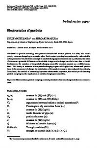
κ2 = 10−17 N A I s ϵ0 k Bc T , g is a boundary value function, δ(r − rj ) denotes the Dirac-delta distribution at atomic position rj [49], and ∂Ω denotes the boundary of a bounded domain Ω satisfying that Ω = D p ∪ D s ∪ Γ. Here, ϵ0 , e c , k B , T, N A , and I s are the permittivity of vacuum, the electron charge, the Boltzmann constant, the absolute temperature, the Avogadro number, and the ionic strength, respectively, and we often select Ω as a box domain or a spherical domain. See Figure 1 for an illustration on the domain partition.

Figure 1: An illustration of protein region D p , interface Γ, and solvent region D s with two species of ions (in red and blue).


182 | Yi Jiang, Yang Xie, Jinyong Ying, Dexuan Xie, and Zeyun Yu When the absolute value of electrostatic potential u is less than linearize (2.1) to obtain a linearized PBE model (LPBE) in the form ⎧ np ⎪ e2c ∑︁ ⎪ ⎪ −ϵ p ∆u(r) = 1010 z j δ(r − rj ), ⎪ ⎪ ϵ0 k B T ⎪ ⎪ j=1 ⎨ −ϵ s ∆u(r) + κ2 u(r) = 0, ⎪ + − ⎪ ⎪ ⎪ u(s+ ) = u(s− ), ε s ∂u(s ) = ε p ∂u(s ) , ⎪ ⎪ ∂n(s) ∂n(s) ⎪ ⎩ u(s) = g(s),

1 over the solvent region D s , we can

r ∈ Dp , r ∈ Ds ,

(2.2)

s ∈ Γ, s ∈ ∂Ω.

To overcome the solution singularity difficulty caused by Dirac-delta distributions, we construct the PBE solution u by using the solution decomposition formula ˜ + Ψ(r) + G(r), u(r) = Φ(r)

r ∈ Ω,

(2.3)

where G is given in the analytical expression G(r) = 1010

np ∑︁ zj e2c 4πϵ0 ϵ p k B T |r − r j |

∀r ≠ rj ,

j = 1, 2, . . . , n p ,

(2.4)

j=1

Ψ is a solution of the following linear interface boundary value problem, ⎧ ∆Ψ(r) = 0, ⎪ ⎪ ⎨ ∂Ψ(s− ) ∂G(s) ∂Ψ(s+ ) + − = ϵp + (ϵ p − ϵ s ) , Ψ(s ) = Ψ(s ), ϵ s ⎪ ∂n(s) ∂n(s) ∂n(s) ⎪ ⎩ Ψ(s) = g(s) − G(s),

r ∈ Dp ∪ Ds , s ∈ Γ,

(2.5)

s ∈ ∂Ω,

˜ is a solution of the following nonlinear interface boundary value problem, and Φ ⎧ ⎪ ⎪ ⎪ ⎪ ⎨ ⎪ ⎪ ⎪ ⎪ ⎩

˜ ∆ Φ(r) = 0, ˜ + κ2 sinh(Φ ˜ + Ψ + G) = 0, −ϵ s ∆ Φ(r) + ˜ − ˜ ˜ + ) = Φ(s ˜ − ), ϵ s ∂ Φ(s ) = ϵ p ∂ Φ(s ) , Φ(s ∂n(s) ∂n(s) ˜ Φ(s) = 0,

r ∈ Dp , r ∈ Ds , s ∈ Γ,

(2.6)

s ∈ ∂Ω.

Clearly, when |u(r)| < 1 for r ∈ D s , (2.6) can also be linearized into the following linear interface problem: ⎧ ˜ ∆ Φ(r) = 0, ⎪ ⎪ [︀ ]︀ ⎪ 2˜ ⎪ ˜ ⎨ −ϵ s ∆ Φ(r) + κ Φ(r) = −κ2 Ψ(r) + G(r) , ˜ − ˜ + ˜ + ) = Φ(s ˜ − ), ϵ s ∂ Φ(s ) = ϵ p ∂ Φ(s ) , ⎪ Φ(s ⎪ ⎪ ∂n(s) ∂n(s) ⎪ ⎩ ˜ Φ(s) = 0,

r ∈ Dp , r ∈ Ds , s ∈ Γ,

(2.7)

s ∈ ∂Ω.

˜ l of the above linear interface problem will be selected as a default initial guess to the solution The solution Φ ˜ Φ of nonlinear interface problem (2.6) in our modified Newton minimization algorithm for solving (2.6). ˜ l of (2.7), we obtain the solution u l of LPBE by the formula Moreover, using the solution Φ ˜ l (r) + Ψ(r) + G(r), u l (r) = Φ

r ∈ Ω.

(2.8)

˜ are twice continuously differentiable within D p and D s . Hence, both (2.5) As shown in [59], both Ψ and Φ and (2.6) are well defined in strong partial derivatives. Therefore, they can be solved numerically by either a finite difference method or a finite element method. On the other hand, from the expression (2.4) of G it can be seen that G has the singularity points at atomic positions rj for j = 1, 2, . . . , n p , implying that the PBE solution u is singular. Due to this reason, the PBE model (2.1) and the LPBE model (2.2) should be redefined by the solution decomposition formulas (2.3) and (2.8), respectively, to make sense in strong partial derivatives.



| 183

Traditionally, the PBE model (2.1) was solved directly after it was modified by substituting each Diracdelta distribution δ(r−rj ) to a numerical approximation function δ h (r−rj ) constructed by a fractional weighted charge assignment scheme based on a grid mesh of domain Ω with mesh size h [32]. Such a modification results in a modified PBE model that is well defined, but it still causes serious difficulties in the calculation of PBE numerical solutions. In fact, due to the fact that u h → u as h → 0, the numerical solution u h of such a modified PBE model may become more and more bumpy a smaller and smaller h is used. Hence, it is necessary for us to use solution decomposition techniques to effectively overcome the difficulty of solution singularity. In the starting version of our web server, two particular PBE solvers are incorporated for users to select. One is the finite element PBE solver proposed in [59]. It is developed based on an unstructured interface-fitted tetrahedral mesh of Ω to fully take advantages of the finite element method in handling the complicated surface shape of interface Γ and the interface conditions. The second one is a novel finite element and finite difference hybrid solver of PBE proposed in [65]. It is constructed based on the Schwarz alternating domain decomposition method and a novel seven-boxes partition of Ω for the purpose of taking advantages of both finite element and finite difference methods. It has been shown to be able to significantly improve the performance of the PBE finite element solver in both CPU time and computer memory amount, especially for large biomolecule cases. Both PBE solvers can guarantee the numerical convergence and numerical stability [59, 65]. One main feature of our PBE solvers is a new modified Newton minimization algorithm for solving (2.6) ˜ While the detailed description of this algorithm can be found in [59], we shortly review it here for clarity. for Φ. After both G and Ψ are calculated, the interface boundary value problem (2.6) is reformulated as the variational minimization problem: ˜ = min J(v), J(Φ) (2.9) v∈M0

where M denotes a finite element function space as a subspace of the usual Sobolev function space H 1 (Ω), M0 is a subspace of the Sobolev function space H01 (Ω), and J is defined by ∫︁ 1 J(v) = a(v, v) + κ2 cosh(Ψ + G + v)dr 2 Ds

with a(u, v) being a bilinear functional given by ∫︁ ∫︁ a(u, v) = ϵ p ∇u · ∇vdr + ϵ s ∇u · ∇vdr. Dp

Ds

˜ (k) }, as follows: The modified Newton minimization algorithm is then defined as a sequence of iterates, {Φ ˜ (k+1) = Φ ˜ (k) + λ k p k , Φ

k = 0, 1, 2, . . . ,

(2.10)

˜ (0) is an initial guess, λ k is a step length, and p k is a search direction defined by the Newton equation: where Φ Find p k ∈ M0 such that

˜ (k) )(p k , v) = −J ′ (Φ ˜ (k) )v J ′′ (Φ

∀ v ∈ M0 .

(2.11)

˜ and J ′′ (Φ) ˜ denote the first and second Fréchet-derivative of J at Φ, ˜ respectively. They can be found Here J ′ (Φ) as follows: ∫︁ ∫︁ ˜ = a(Φ, ˜ v)+κ2 sinh(Ψ+G+Φ)vdx, ˜ ˜ ˜ J ′ (Φ)v J ′′ (Φ)(p, v) = a(p, v)+κ2 cosh(Ψ+G+Φ)pvdx ∀p, v ∈ H01 (Ω). Ds

Ds

As a descent search method, our modified Newton minimization algorithm can be shown to converge globally [15, 44].


184 | Yi Jiang, Yang Xie, Jinyong Ying, Dexuan Xie, and Zeyun Yu Furthermore, we find that the Newton equation (2.11) can be rewritten in the strong partial derivative form as a linear interface boundary value problem as follows [65]: ⎧ ˜ −∆p(r) = ∆ Φ(r), r ∈ Dp , ⎪ ⎪ ⎪ 2 ⎨ −ϵ s ∆p(r) + κ2 cosh(Ψ + G + Φ)p(r) ˜ ˜ ˜ = ϵ s ∆ Φ(r) − κ sinh(Ψ + G + Φ), r ∈ Ds , (2.12) ˜ −) ˜ +) ∂p(s+ ) ∂p(s− ) ∂ Φ(s ∂ Φ(s + − ⎪ p(s ) = p(s ), ϵ − ϵ = ϵ − ϵ , s ∈ Γ, s p p s ⎪ ∂n(s) ∂n(s) ∂n(s) ∂n(s) ⎪ ⎩ p(s) = 0, s ∈ ∂Ω. Due to this equivalence, our modified Newton minimization algorithm can also be implemented based on the finite difference approach. Obviously, the performance of our PBE finite element solver is mainly determined by that of a linear iterative method for solving the linear interface boundary value problem (2.5) and the Newton equation (2.11) or (2.12). In SDPBS, each involved linear system generated from finite element approximation is solved by the preconditioned conjugate gradient method (PCG) with incomplete LU preconditioning (PCG-ILU) until the absolute and relative residue errors less than a given tolerance (10−7 by default). Here an unstructured interface fitted tetrahedral mesh has been used to well approximate the interface Γ. Such a finite element solver can yield a numerical solution of PBE in high accuracy in comparison to the case of using an uniform finite difference mesh [29]. However, it also causes geometric multigrid techniques no longer to work, and requires extra memory locations to store the mesh data. In addition, the nonzero entries of the coefficient matrix of each involved linear system are required to store for the finite element solver. These shortcomings motivated us to develop the PBE hybrid solver to fully take advantages of both finite element and finite difference methods. Our PBE hybrid solver is a modification of our PBE finite element solver. It uses a new seven-box iterative scheme for solving Ψ and search direction p k based on a novel seven overlapped box partition of a cubic domain Ω with the central box containing D p surrounding by other six neighboring boxes. The finite element method is then applied to the central box to deal with the interface problem while the finite difference method is used to solve a Poisson like boundary value problem defined on each neighboring box. Using an uniform Cartesian mesh, we developed a PCG with multigrid V-cycle preconditioning to solve each system of finite difference equations optimally in the sense that the convergence rate is independent of the mesh size h. Consequently, a hybrid solver is obtained to solve PBE more efficiently than the finite element solver. See [65] for the details of our PBE hybrid solver. ˜ (0) can be selected as zero or a solution of a linearized equation (2.7) [35], In SDPBS, the initial iterate Φ (k) ˜ is output as a numerical solution of (2.6) provided that and the kth iterate Φ ˜ (k) − Φ ˜ (k−1) || < ϵ, ||Φ

(ϵ = 10−5 and || · || is a Euclidean vector norm by default).

(2.13)

3 Electrostatic solvation and binding free energy calculation One important application of PBE is to predict the solvation free energy ∆E of a biomolecule. Usually, ∆E is split as ∆E = E es + E np , where E es and E np denote the polar and non-polar parts of ∆E, respectively. E np reflects some non-electrostatic properties depending on surface area, volume, hydrodynamic pressure, and Lennard-Jones potential [56]. Its calculation will be added to SDPBS in the next version of our web server. In the implicit solvent continuum dielectric approach, the polar part E es is commonly estimated in the units of kilocalories per mole (kcal/mol) by ∫︁ NA kB T ρ f (r)(u sol − u ref )(r)dr, (3.1) E es = 4184 2e c Ω

where u sol and u ref denote the electrostatic potential functions in the solvent and reference states, respectively, and ρ f denotes the fixed charge density function. However, in the case of a protein, we have ρ f =



| 185

∑︀n p e c j=1 z j δ(r − rj ), which causes the solution singularity difficulty. To avoid this difficulty, we have used the solution decomposition (2.3) to reformulate (3.1) as the new formula for computing the electrostatic solvation free energy: np ]︀ NA k T ∑︁ [︀ ˜ j) . E es = z j Ψ(rj ) + Φ(r · B (3.2) 4184 2 j=1

In particular, when the ionic strength I s = 0, the solvent becomes the pure water, implying from (2.6) that ˜ = 0. Hence, the electrostatic solvation free energy for a protein in water can be simply calculated by Φ E es

np k B T ∑︁ NA · z j Ψ(rj ). = 4184 2

(3.3)

j=1

Figure 2: A cross section view of a tetrahedral mesh of the central box, which is used to define the PBE hybrid solver, for a protein (PDB: ID 1C4K). Here the protein region D p is colored in blue.

As another important application, PBE is widely used to compute a binding free energy, E b , to study the salt dependance of two molecules A and B binding as a complex C [8, 20, 52]. In SDPBS, we calculate E b by E b (I s ) = E(C, I s ) − E(A, I s ) − E(B, I s ),

(3.4)

where E(X, I s ) denotes an electrostatic free energy of molecule X from the water state to the salt solution state with the ionic strength I s ∈ (0, 1). Since the sum of G and Ψ gives the potential in the water state, E(X, I s ) can be simply computed by np NA k T ∑︁ ˜ · B z j Φ X,I s (rj ), (3.5) E(X, I s ) = 4184 2 j=1

˜ X,I s denotes a solution of the nonlinear problem (2.6) for molecule X in the salt solution with ionic where Φ strength I s . By variable change ξ = ln I s (or set ξ = log10 I s ), chemical experiments have observated that the binding free energy E b can be written as a linear function of ξ with the slope m on an interval [a1 , a2 ] of ξ [41]: E b = mξ + b,

a1 ≤ ξ ≤ a2 .

(3.6)

Computationally, the slope m can be predicted in the following three steps: 1. Select ξ j = a1 + jτ for j = 0, 1, 2, . . . , l, with τ > 0 and l being the largest number satisfying a1 + lτ ≤ a2 . 2. Calculate binding energies E b (I s,j ) with I s,j = e ξ j for j = 0, 1, 2, . . . , l by a PBE solver. 3. Predict m as the slope of a best fitted line determined by the set of computed binding energies.


186 | Yi Jiang, Yang Xie, Jinyong Ying, Dexuan Xie, and Zeyun Yu

Figure 3: An illustration of our web-server framework.

4 Framework of SDPBS web server In this section, we describe a framework of our SDPBS web server. As illustrated in Figure 3, our SDPBS web server contains the following four major components: 1. The SDPBS solver library. Currently, it contains two PBE solvers reported in [59, 65]. 2. An application toolkit for biochemical and biophysical analysis and applications. It computes various biophysical quantities in terms of electrostatic potentials such as electrostatic solvation free energies, binding free energies, and ionic concentrations. 3. A web-based tool for visualizing PBE numerical solutions and application results. It can visualize biomolecular structures, electrostatic potential distribution on a molecular surface, and iso-surfaces of PBE numerical solutions, as well as tetrahedral finite element meshes on the web server directly. 4. A client-server interactive graphic user interface for inputing data and parameters, monitoring the whole calculation process in real time, and visualizing numerical solutions and application results. Our goal is to produce an integrated biomolecular analysis tool with minimum client software and hardware requirements such that our SDPBS software package can be easy to access for the scientific and educational communities. Equipped with a new web-based visualization tool and a client-server interactive graphic user interface, end users can carry out biomolecular analysis according to the PBE numerical results generated from SDPBS directly on the web server.

4.1 SDPBS software development In order to take advantage of the efficiency of compiled languages and the usability, maintainability, and interoperability of a high level scripting language, we wrote the software package SDPBS in a mixture of C++, C, Fortran, and Python. The state-of-the-art finite element library DOLFIN [37] from the FEniCS project was employed to implement our finite element solvers. To solve each system of finite element linear equations, we directly called the PCG-ILU iterative algorithm from the scientific computation toolkit PETSc [5, 6]. We developed a new interface-fitted tetrahedral mesh generator, called GAMer II, as an extension of a molecular surface and volumetric mesh generation program package, called GAMer [66]. With GAMer II, we can generate tetrahedral meshes for a rectangular or spherical domain of Ω and three molecular interfaces — the Gaussian surface, the solvent-excluded surface (SES), and the solvent-accessible surface (SAS) [64, 66]. Furthermore, we wrote a program in C to adaptively generate the seven overlapped boxes of Ω and a mesh of the central box that mixes an uniform Cartesian mesh with an unstructured finite element mesh for our PBE hybrid solver as illustrated in Figure 2. In GAMer II, the C++ program TetGen (http://wias-berlin.de/software/tetgen/1.5/index. html) was adopted to generate tetrahedral meshes. All the Fortran, C and C++ programs were converted into Python extension modules by the Fortran-to-Python interface generator f2py (http://cens.ioc.ee/projects/



| 187

f2py2e/) and the software development tool SWIG (http://www.swig.org). To merge well with this web server, we wrapped SDPBS as one independent Python library. The Gaussian surface is a default selection for generating the interface Γ in SDPBS. According to recent studies [36], we can produce a Gaussian surface similar to SES through properly setting the two controlling parameters (the decay rate and isovalue) of the Gaussian surface option.

4.2 An interactive client-server architecture The web server follows a standard client-server architecture, as illustrated in Figure 3. Parameter input, results output, and visualization tools comprise the front end or client side of the server, while the SDPBS solver library and application toolkit comprise the back end or server side of the server. These two divisions communicate with each other through an internet connection. The front end provides a 3D visualization environment for user’s manipulations (see below for detail) and serves as a graphical user interface for parameter-tuning. The interface takes PDB or PQR file(s), which indicate biomolecular structure information, as input, and allows end users to adjust the parameters of our PBE solvers to control the quality of PBE numerical solutions and other biophysical quantities to be predicted. These parameters enable users to customize the performance of our SDPBS by changing dielectric constants, directing mesh quality, and adjusting linear solver accuracies. All the parameters are grouped in a file that can be automatically loaded during calculation. In order to provide a neat interface appearance and simplify the usage of SDPBS, only the most important parameters are exposed on the user-facing page. All the parameters have default values, which can be adjusted if necessary. The front end’s graphical user interface is implemented with a combination of HTML5, CSS, JavaScript, and PHP. The back end of the software package takes charge of all numerical tasks involving heavy PBE calculations. As the kernel computation module, SDPBS itself is organized as a complete and independent software package, serving as a program library to efficiently solve PBE. Once all required input parameters are received from the user interface, SDPBS will automatically invoke appropriate library functions to generate finite element meshes, assemble and solve linear systems, calculate and save results, and perform applications such as solvation and binding free energy calculations. A separate LAMP (Linux, Apache, MySQL, PHP) server acts as an intermediary between the client side and the computational back end. It accepts and sanitizes parameter settings from the client, relays them to the computational node, and sends calculation results back to the client via visualization data and a download link to a zipped file containing output files. The user may specify several output formats for download. These files can then be used in external visualization software, such as VMD and ParaView.

4.3 A web-based visualization tool Our program uses WebGL (Web Graphics Library) to render molecular models on the front end. WebGL is a graphical library, equipped with a pure JavaScript, hardware-accelerated and object-oriented programming environment, which allows users to visualize and interact instantly with molecular data in any modern desktop or mobile web browser. Currently, WebGL is supported by the most popular web browsers (including Chrome, FireFox, Safari and Window Edge, etc.) without needing plugins. Thanks to these features, the users of our SDPBS can acquire high quality visualization in a convenient and interactive environment, and are able to access the application from anywhere through the internet with minimum software and hardware requirements. With WebGL, our package now supports displaying finite element meshes and electrostatic potentials. Most notably, as a direct result of solving PBE, the electrostatic potential can be plotted as biomolecular surface mappings. Users can also translate, rotate, and zoom these geometric objects via simple mouse clicks. The visualization component of the website will be continually updated after initial publication; future functionalities are planned to include: the ability to superimpose electrostatic potential mappings over the


188 | Yi Jiang, Yang Xie, Jinyong Ying, Dexuan Xie, and Zeyun Yu biomolecular structure; the ability to view iso-surfaces or slice views of electrostatic potential and ionic concentration results; and a control panel that allows users to adjust detailed view settings such as plotting methods, lighting and coloring schemes.

5 Numerical tests and validations In this section, we present some numerical results produced from SDPBS to demonstrate the efficiency, stability and some visualization features of the SDPBS web server. For simplicity, we used the original PDB files downloaded from the Protein Data Bank (PDB) (http://www.rcsb.org/), and then converted them to PQR files by the program tool PDB2PQR (http://www.poissonboltzmann.org/pdb2pqr/) [16] to get the atomic coordinates, atomic charges, atomic radii, and the hydrogen atoms that are missed in the PDB file. All the tests were done on our Mac Pro Workstation with 3.7 GHz Quad-Core Intel Xeon E5 processor and 64 GB memory. Unless explicitly mentioned, we used the following parameter values: ϵ p = 2.0, ϵ s = 80.0, I s = 0.1, and T = 298.15, and generated the biomolecular surface using the Gaussian function.

5.1 Performance of SDPBS for proteins In these tests, we solved the PBE and LPBE models using both the PBE finite element solver and PBE hybrid solver for twelve proteins with the numbers of atoms up to 11,439. In the calculations, we set the boundary value function g = 0, selected the domain Ω as a cubic box with side length L = 2diam(D p ), and measured the CPU time in seconds. Here, diam(D p ) = max{|r − r′ | | r, r′ ∈ D p }, which is called the diameter of protein region D p . In the test, all the parameters were set as their default values (see Appendix) except that MeshSizeUpperLimit was set as 20000 and MeshSizeLowerLimit was set as 500, respectively, for the purpose of reducing the number of mesh points. The numerical results are reported in Table 1. From Table 1 we can see that both PBE solvers took only about 5 to 43 seconds for the proteins on a mesh with up to 50000 mesh points, showing the high efficiency of our SDPBS web server in the calculation of electrostatic solvation free energy E es as defined in (3.2).

5.2 Validation tests on SDPBS ˜ h } of (2.5) and (2.6), calculated on a sequence of Clearly, the numerical solution sequences {Ψ h } and {Φ meshes of Ω, lead to a sequence {E es,h } of approximations to electrostatic solvation free energy E es . For a convergent and numerically stable PBE solver, the sequence {E es,h } should vary around E es in a small range as h → 0. Hence, this property can be used to verify the numerical behavior of a PBE solver since the exact solution of PBE is usually unknown in the case of protein calculation. To validate the convergence of our SDPBS in the calculation of E es , we calculated E es by the formula (3.2) for a set of 100 proteins, which we selected from a protein database maintained by Prof. Ray Luo on his home page http://rayl0.bio.uci.edu/rayl/. In these tests, we repeated the calculation of E es using six successively refined meshes for each protein. For short, these computed values of E es were reported in Figure 4a in terms of their averages over the 100 proteins. Since the analytical value of E es is unknown, we took the value of E es from the finest mesh as the reference to calculate the relative errors of other five computed values of E es . We then reported them in Figure 4b in the averages of these relative errors over the 100 proteins. Here, the averaged numbers of mesh points over the 100 meshes for the six mesh sets are 21362, 35036, 43856, 56716, 137681, 239518, the averaged mesh sizes of h max are 21.78, 16.04, 12.30, 10.24, 8.78, 7.68 respectively, and the averaged mesh sizes of h min are 0.15 for the six mesh sets. Here h max = maxT∈T diam(T), and h min = minT∈T diam(T) with diam(T) denoting the diameter of a tetrahedron T. All the parameters were set as their default values (see Appendix) except that DIM_SCALE =


Protein PDB ID 2LZX 1AJJ 1FXD 1HPT 4PTI 1SVR 1A63 1CID 1A7M 2AQ5 1F6W 1C4K

Number of atoms 488 513 811 852 892 1, 433 2, 065 2, 783 2, 803 6, 024 8, 243 11, 439

34, 717 35, 795 36, 035 36, 968 36, 480 39, 038 41, 085 39, 773 40, 285 47, 064 51, 048 59, 768

Nh

Tetrahedral mesh h max CPU time (h min ) FE Hybrid 8.51 (0.36) 4.75 2.35 8.88 (0.23) 5.18 2.73 9.79 (0.23) 5.52 3.08 10.27 (0.24) 6.14 3.52 10.55 (0.34) 5.67 3.04 11.75 (0.19) 7.06 4.33 14.92 (0.22) 9.21 6.26 17.80 (0.25) 8.67 5.81 18.63 (0.34) 8.96 5.88 15.88 (0.29) 14.03 10.99 19.17 (0.28) 19.42 15.64 26.35 (0.14) 27.40 23.28

Linearized PBE CPU time Solvation energy FE Hybrid FE Hybrid 5.71 3.58 −210.49 −210.49 6.19 4.09 −306.16 −306.16 6.73 4.61 −1313.23 −1313.23 7.42 5.15 −115.12 −115.12 6.97 4.65 −322.46 −322.46 8.86 6.54 −272.23 −272.23 11.65 9.12 −456.43 −456.43 11.54 8.83 −298.85 −298.85 11.90 9.04 −463.06 −463.06 20.42 17.68 −879.53 −879.53 28.61 25.25 −908.49 −908.49 41.86 38.95 −3114.53 −3114.53

Nonlinear PBE CPU time Solvation energy FE Hybrid FE Hybrid 17.14 9.70 −217.22 −217.22 21.67 13.84 −317.23 −317.23 21.17 10.27 −1340.04 −1340.04 21.79 12.16 −122.99 −122.99 20.39 9.89 −331.47 −331.47 19.05 15.56 −291.61 −291.61 32.13 20.39 −487.50 −487.50 28.52 19.74 −322.87 −322.87 32.33 20.72 −486.62 −486.62 42.01 31.72 −923.08 −923.08 51.04 35.86 −967.58 −967.58 72.54 62.92 −3243.13 −3243.13

Table 1: A comparison of the performance of our PBE finite element solver (FE) with that of our PBE hybrid solver (Hybrid) in solving the linearized PBE and the nonlinear PBE for 12 proteins in CPU runtime (seconds). Here, N h is the number of mesh points for a tetrahedral mesh T of Ω, h max = maxT∈T diam(T), and h min = minT∈T diam(T) with diam(T) denoting the diameter of a tetrahedron T.

SDPBS Web Server for Electrostatics of Biomolecules | 189


−1040

1.50E−2

PBE Finite Element Solver PBE Hybrid Solver

PBE Finite Element Solver PBE Hybrid Solver

Averaged Relative Error

Averaged Solvation Energy (kcal/mol)


−1043.76

−1046.71 −1048.07

−1052.14 −1053.30 −1055

1.03E−2

6.29E−3

1.37E−3

21362

35036

43856

56716

137681

0

239518

21362

Averaged Number of Mesh Points

(a) Electrosatic solvation energy

35036

43856

56716

137681

Averaged Number of Mesh Points

(b) Relative error

Figure 4: A validation of the convergence behavior of our PBE finite element and hybrid solvers in the calculation of electrostatic solvation free energy E es , defined in (3.2), for 100 proteins downloaded from the website http://rayl0.bio.uci.edu/rayl/. In Plot (b), the relative errors were calculated by using the values of E es on the finest mesh as the references.

1.99, PRO_PART was set as 6, 8, 10, 12, 14, 16, MIN_RATIO was set as 1.5, 1.2, 1.2, 1.2, 1.1, 1.1, and MAX_VOLUME was set as 1000, 100, 10, 5, 1, 0.5 for for the six sets of meshes, respectively. From Figure 4 we can see that the values of E es produced by the finite element solver were almost the same as those by the hybrid solver, which varied in a very small range, and their relative error values changed less than 0.01 only as the averaged number of mesh points was increased from 21,362 to 239,518. These tests confirm the convergence and numerical stability of our SDPBS web server in the calculation of electrostatic solvation free energy E es .

5.3 Tests on binding free energy calculation Our SDPBS web server provides the end user with a function to calculate the binding free energy. As an example, we did tests on this function using a DNA-drug complex (PDB ID: 1D86). The PQR files were the same as the ones used in [18]. An experimental value of a scaled dimensionless slope, m s , was determined chemically as m s = −1.51 [9, Table 3]. We converted it to a value of m, m = 0.8946 kcal/mol, by the formula m = −m s N A k B T/4184. In our numerical tests, we set τ = 0.2 and l = 11 for a1 = −3 and a2 = −1, which corresponds to 0.05 ≤ I s ≤ 0.37. We then constructed three meshes with 259903, 261512, and 233983 mesh points for the DNA-drug complex, DNA, and drug, respectively. Here we used the same parameter values for the complex, DNA and drug, which were set as default values except that DIM_SCALE = 1.99, MIN_RATIO = 1.2, PRO_PART = 12, OVER_POW = 2, DOM_RATIO = 5, and MAX_VOLUME = 100 for mesh generations. The calculated values of binding free energy E b on the SDPBS web server were plotted in Figures 5, together with their best fitted line determined by the linear least square fitting regression scheme. The slope of this best fitted line was found to be 0.8886 ± 0.003, which is close to the experimental slop m = 0.8946. Remarkably, the deviation is only 0.003, implying that all the computed binding energies almost lie on a straight line. Hence, our test results agree well with the experimental observation that the binding free energy E b has a linear relationship with the variable ξ = ln I s (or log I s ) as given in (3.6).


SDPBS Web Server for Electrostatics of Biomolecules |

191

Binding Free Energy (kcal/mol)

540 Calculated binding free energy Linear least square fitting line 539.5

539

538.5

538

537.5

−3.0

−2.5

−2.0

−1.5

−1.0

ln(I s ) Figure 5: A best-fitted line determined by the 11 values of binding free energy E b computed from the SDPBS web server for a DNA-drug complex (PDB ID: 1D86). Here, the best-fitted line has the slope 0.8886 ± 0.003, which is close to the experimental slop 0.8946 reported in [9, Table 3], and E b is defined in (3.6).

Figure 6: Two iso-surfaces of the electrostatic potential generated according to the PBE numerical solution for a protein (PDB ID: 1SVR). Here, the iso-surfaces defined by u(r) = −50 and u(r) = 50 (in units: k B T/e c ) are colored in red and green, respectively, and the protein structure is plotted in sticks and balls.

Figure 7: Visualization of the electrostatic potential and finite element mesh on the molecular surface of a protein (PDB ID: 1SVR) produced from the SDPBS web server.

5.4 Visualizations of PBE solution on molecular surface In a future update, we plan to add a functionality to the web-based visualization tool that allows users to view an iso-surface (known as equipotential surface) of the electrostatic potential directly on the the web server. As a target example, Figure 6 displays two iso-surfaces of the electrostatic potential – the PBE numerical solution for a protein (PDB ID: 1SVR), which were produced from an existing visualization package. Figure 7 displays two graphs extracted from the visualization window of our SDPBS web server. Here, different colors stands for different values of the PBE numerical solution, and the graphics were rendered directly from the PBE numerical solution on the finite element mesh without doing any additional interpolation, since a finite element solution has been well defined over the whole domain Ω. They were plotted by


192 | Yi Jiang, Yang Xie, Jinyong Ying, Dexuan Xie, and Zeyun Yu using our visualization tool according to the PBE numerical solution and mesh data generated from SDPBS for a protein (PDB ID: 1SVR). The picture on the left side of Figure 7 visualizes the electrostatic potential on the molecular surface of the protein. With our web-based visualization tool, we can view the electrostatic potential — the PBE solution — over different across sections in different rotation angles. The other picture of Figure 7 demonstrates a zoom-in view of the electrostatic potential to closely examine the behavior of PBE numerical solution. It also displays the triangular mesh of the molecular surface produced from our finite element mesh generation program on a local surface area. Acknowledgement: This work was partially supported by the National Science Foundation, USA, through grant DMS-1226259. Conflict of interest: Authors state no conflict of interest.

Appendix: SDPBS parameters and usages In this appendix, we list the default values and usages of SDPBS parameters as follows. 1. Parameters for PBE definition ϵ p : Dielectric constant for protein region D p . Range: 1.0–20.0 (2.0 by default). ϵ s : Dielectric constant for protein region D s . Range: 1.0–20.0 (80.0 by default). T: Absolute temperature in Kelvins. Range: 260–320 ( 298.15 by default). Is : Ionic strength in moles per liter. Range: 0.0–2.0 ( 0.1 by default). Bdy_Cond_Option: Specifies the Dirichlet boundary condition. “Zero": zero boundary value function (default); “MDH": multiple Debye-Huckel boundary value function. Hyper_bound : Specifies upper bound for the values of the hyperbolic function to avoid the blow-up problem. Range: 50.0–100.0 (85.0 by default). ModelType: Specifies a linear or nonlinear model for calculation. “Nonlinear": nonlinear PBE (default); “Linear": linear PBE. 2. Parameters for mesh generation Domain_flag: SurfMethod: IsoValue: Blobbyness: Probe_radius: DIM_SCALE:

DomainRatio: OutSurfLayer:

Selects the geometric shape of computational domain Ω (for finite element solver only). 1: cubic domain (default); 2: spherical domain. Selects the interface surface Γ. 1: Gaussian surface (default); 2: SES; 3: SAS. Level set parameter of Gaussian function for defining the Gaussian surface. Range: 0.1–3.00 (1.0 by default). Blurring blobbyness parameter of Gaussian function for defining the Gaussian surface. Range: −1.0– − 0.1; (−0.2 by default). Radius of the probe rolling ball for SES and SAS surfaces. Range: 1.0–2.0 (1.4 by default). Marching cube density parameter for generating the protein domain D p . A larger value causes more surface mesh nodes to generate. Range: 0.01–3.00 (1.5 by default). Diameter ratio of the whole domain Ω to the protein domain D p . Range: 1.0–20.0 (2.0 by default). Number of mesh nodes on the whole domain boundary (4OutSurfLayer + 2). Works for Domain_flag = 2 only. Range: 4–8 (6 by default).



193

Coarsen_rate:

Controls the coarsening process of the triangular surface mesh. A larger value causes more surface mesh nodes to delete. Range: 0.1–0.4 (0.3 by default). MeshSizeUpperLimit: Upper limit on the mesh node number of the triangular surface mesh. Range: 5000–100000 (80000 by default). MeshSizeLowerLimit: Lower limit on the mesh node number of the triangular surface mesh. Range: 500–20000 (10000 by default). MinRatio: Smallest allowable ratio R/L for each tetrahedron, where R is the radius of the circumsphere of a tetrahedron, and L is the length of the shortest edge of the tetrahedron. Range: 1.0–2.0; (1.8 by default) ˚ 3 ) of a tetrahedron (no restriction if set as 0). MaxVolume: Largest allowable volume (A Range: 0–10000 (10000 by default). 3. Parameters for hybrid solvers Pro_Part: Mesh partition number of the central cubic box along each side. Range: 8 or 16 (default). Over_Pow: Number of overlapping grid layers of the central box mesh (2OVER_POW ). Range 0–3 (1 by default). 4. Parameters for linear iterative solvers ElementDegree: LinearSolverType:

Specifies a finite element degree. Range: 1 (default); 2; 3. Selects a linear iterative solver. “gmres": Generalized Minimum Residual method (default); “cg": Conjugate Gradient method; “bicgstab": Bi-conjugate Gradient method; “direct": LU factorization method. Preconditioner: Selects a preconditioning method for solving a linear system. “ilu": Incomplete LU decomposition (default); “icc": Incomplete Cholesky; “pestc_amg": Algebraic multigrid. relative_tolerance: Tolerance of relative residual of linear solver. Range: 10−8 –10−4 (10−8 by default). absolute_tolerance: Tolerance of absolute residual of linear solver. Range: 10−8 –10−4 (10−8 by default). maximum_iterations: Maximum number of iterations for a linear solver. Range: 1000–10000 (5000 by default). nonzero_initial_guess: Specifies an initial guess for a linear iterative solver. “Yes: Use a nonzero initial guess (default); “No": Use zero as an initial guess. monitor_convergence: Specifies to output the iterative information of a linear iterative solver. “Yes": Output the iterative information; “No": No any output (default). 5. Parameters for nonlinear iterative solvers Init_Guess_Option:

Specifies an initial guess for solving a system of nonlinear equations. “Zero": Use zero as an initial guess; “Linear": Use a nonzero initial guess. newton_tolerance : Specifies a tolerance for the stopping criteria for a nonlinear iterative method. ||Φ(k) − Φ(k−1) ||2 < newton_tolerance. Range: 10−7 –10−3 (10−7 by default). box_iter_tol : Specifies a tolerance for the stopping criteria for the hybrid box iterative method. ||Ψ (j) − Ψ (j−1) ||2 < box_iter_tol for solving Ψ. Range: 10−8 –10−4 ; (10−8 by default). 6. Parameters for result output OutputHeader: WRITE_POT_DAT: WRITE_MESH_XML: WRITE_POT_PVD: WRITE_POT_OPENDX:

Output file name prefix. Range: 1–20 characters. Specifies to save PBE numerical results to a plain text file. “Yes": Save the results (default); “No": Do not save. Specifies to save volumetric mesh data to a file in xml format. “Yes": Save the data; “No": Do not save (default). Specifies to save PBE numerical results to a file in pvd format. “Yes": Save the results; “No": Do not save (default). Specifies to save PBE numerical results to a file in opendx format. “Yes": Save the results; “No": Do not save (default).



References [1] [2] [3] [4] [5] [6] [7] [8] [9]

[10] [11] [12] [13] [14] [15] [16] [17] [18] [19] [20] [21] [22] [23] [24] [25] [26] [27] [28] [29]

J. Ahrens, B. Geveci, and C. Law. ParaView: An end user tool for large data visualization. In C. Hansen and C. Johnson, editors, The Visualization Handbook, pages 717–731. Academic Press, 2005. N. Baker, M. Holst, and F. Wang. Adaptive multilevel finite element solution of the Poisson–Boltzmann equation II. Refinement at solvent-accessible surfaces in biomolecular systems. Journal of Computational Chemistry, 21(15):1343–1352, 2000. N. A. Baker, D. Sept, S. Joseph, M. Holst, and J. A. McCammon. Electrostatics of nanosystems: Application to microtubules and the ribosome. Proc. Natl. Acad. Sci. USA, 98(18):10037–10041, 2001. N.A. Baker, D. Sept, M.J. Holst, and J.A. McCammon. The adaptive multilevel finite element solution of the Poisson-Boltzmann equation on massively parallel computers. IBM Journal of Research and Development, 45(3.4):427–438, 2001. S. Balay, J. Brown, K. Buschelman, V. Eijkhout, W.D. Gropp, D. Kaushik, M.G. Knepley, L.C. McInnes, B.F. Smith, and H. Zhang. PETSc users manual. Technical Report ANL-95/11 - Revision 3.1, Argonne National Laboratory, 2010. S. Balay, J. Brown, K. Buschelman, W.D. Gropp, D. Kaushik, M.G. Knepley, L.C. McInnes, B.F. Smith, and H. Zhang. PETSc Web page, 2012. http://www.mcs.anl.gov/petsc. Donald Bashford and Martin Karplus. pKa’s of ionizable groups in proteins: atomic detail from a continuum electrostatic model. Biochemistry, 29(44):10219–10225, 1990. C. Bertonati, B. Honig, and E. Alexov. Poisson-Boltzmann calculations of nonspecific salt effects on protein-protein binding free energies. Biophysical Journal, 92(6):1891–1899, 2007. Kenneth J Breslauer, David P Remeta, Wan-Yin Chou, Robert Ferrante, James Curry, Denise Zaunczkowski, James G Snyder, and Luis A Marky. Enthalpy-entropy compensations in drug-DNA binding studies. Proceedings of the National Academy of Sciences, 84(24):8922–8926, 1987. D. Chen, Z. Chen, C. Chen, W. Geng, and G. Wei. MIBPB: A software package for electrostatic analysis. Journal of Computational Chemistry, 32(4):756–770, 2011. L. Chen, M. J. Holst, and J. Xu. The finite element approximation of the nonlinear Poisson-Boltzmann equation. SIAM Journal on Numerical Analysis, 45(6):2298–2320, 2007. I.L. Chern, J.G. Liu, and W.C. Wang. Accurate evaluation of electrostatics for macromolecules in solution. Methods and Applications of Analysis, 10(2):309–328, 2003. M. E. Davis, J. D. Madura, B. A. Luty, and J. A. McCammon. Electrostatics and diffusion of molecules in solution: Simulations with the University of Houston Browian dynamics program. Comp. Phys. Comm., 62:187–197, 1991. M. E. Davis and J. A. McCammon. Solving the finite difference linearized Poisson-Boltzmann equation: A comparison of relaxation and conjugate gradient methods. J. Comp. Chem., 10:386–391, 1989. J. E. Dennis, Jr. and R. B. Schnabel. Numerical Methods for Unconstrained Optimization and Nonlinear Equations, volume 16 of Classics in Applied Mathematics. SIAM, Philadelphia, PA, 1996. T.J. Dolinsky, J.E. Nielsen, J.A. McCammon, and N.A. Baker. PDB2PQR: An automated pipeline for the setup of Poisson– Boltzmann electrostatics calculations. Nucleic Acids Research, 32(suppl 2):W665, 2004. David Eisenberg and Andrew D McLachlan. Solvation energy in protein folding and binding. Nature, 319:199 – 203, 1986. Marcia O Fenley, Robert C Harris, B Jayaram, and Alexander H Boschitsch. Revisiting the association of cationic groovebinding drugs to DNA using a Poisson-Boltzmann approach. Biophysical Journal, 99(3):879–886, 2010. F. Fogolari, A. Brigo, and H. Molinari. The Poisson-Boltzmann equation for biomolecular electrostatics: A tool for structural biology. J. Mol. Recognit., 15(6):377–392, 2002. C. García-García and D.E. Draper. Electrostatic interactions in a peptide-RNA complex. J. Mol. Biol., 331(1):75–88, 2003. Weihua Geng and Robert Krasny. A treecode-accelerated boundary integral Poisson-Boltzmann solver for electrostatics of solvated biomolecules. J. Comput. Phys., 247:62–78, 2013. Weihua Geng, Sining Yu, and Guowei Wei. Treatment of charge singularities in implicit solvent models. The Journal of Chemical Physics, 127(11):114106, 2007. M.K. Gilson, A. Rashin, R. Fine, and B. Honig. On the calculation of electrostatic interactions in proteins. Journal of Molecular Biology, 184(3):503–516, 1985. M. Holst, N. Baker, and F. Wang. Adaptive multilevel finite element solution of the Poisson-Boltzmann equation I: Algorithms and examples. J. Comput. Chem., 21:1319–1342, 2000. M. Holst, J. A. McCammon, Z. Yu, Y. Zhou, and Y. Zhu. Adaptive finite element modeling techniques for the Poisson-Boltzmann equation. Communications in Computational Physics, 11(1):179–214, 2012. B. Honig and A. Nicholls. Classical electrostatics in biology and chemistry. Science, 268:1144–1149, May 1995. W. Humphrey, A. Dalke, and K. Schulten. VMD: Visual molecular dynamics. Journal of Molecular Graphics, 14(1):33–38, 1996. R.M. Jackson and M.J.E. Sternberg. A continuum model for protein-protein interactions: Application to the docking problem. Journal of Molecular Biology, 250(2):258–275, 1995. Y. Jiang, J. Ying, and D. Xie. A Poisson-Boltzmann equation test model for protein in spherical solute region and its applications. Molecular Based Mathematical Biology, 2:86–97, 2014. Open Access.



195

[30] Sunhwan Jo, Miklos Vargyas, Judit Vasko-Szedlar, Benoît Roux, and Wonpil Im. PBEQ-solver for online visualization of electrostatic potential of biomolecules. Nucleic Acids Research, 36(suppl 2):W270–W275, 2008. [31] John G Kirkwood and Jacques C Poirier. The statistical mechanical basis of the Debye–hüekel theory of strong electrolytes. The Journal of Physical Chemistry, 58(8):591–596, 1954. [32] Isaac Klapper, Ray Hagstrom, Richard Fine, Kim Sharp, and Barry Honig. Focusing of electric fields in the active site of cu-zn superoxide dismutase: Effects of ionic strength and amino-acid modification. Proteins: Structure, Function, and Bioinformatics, 1(1):47–59, 1986. [33] Lev Davidovich Landau and EM Lifshitz. Statistical physics, part I. Course of Theoretical Physics, 5:468, 1980. [34] J. Li and D. Xie. An effective minimization protocol for solving a size-modified Poisson-Boltzmann equation for biomolecule in ionic solvent. International Journal of Numerical Analysis and Modeling, 12(2):286–301, 2015. [35] J. Li and D. Xie. A new linear Poisson-Boltzmann equation and finite element solver by solution decomposition approach. Communications in Mathematical Sciences, 13(2):315–325, 2015. International Press. [36] Tiantian Liu, Minxin Chen, and Benzhuo Lu. Parameterization for molecular gaussian surface and a comparison study of surface mesh generation. Journal of molecular modeling, 21(5):1–14, 2015. [37] A. Logg, K.-A. Mardal, and G. N. Wells, editors. Automated Solution of Differential Equations by the Finite Element Method, volume 84 of Lecture Notes in Computational Science and Engineering. Springer Verlag, 2012. [38] B. Lu, Y. Zhou, M.J. Holst, and J.A. McCammon. Recent progress in numerical methods for the Poisson-Boltzmann equation in biophysical applications. Commun. Comput. Phys., 3(5):973–1009, 2008. [39] Benzhuo Lu, Xiaolin Cheng, and J Andrew McCammon. “New-version-fast-multipole-method” accelerated electrostatic calculations in biomolecular systems. Journal of Computational Physics, 226(2):1348–1366, 2007. [40] Ray Luo, Laurent David, and Michael K Gilson. Accelerated Poisson–Boltzmann calculations for static and dynamic systems. Journal of Computational Chemistry, 23(13):1244–1253, 2002. [41] Gerald S Manning. The molecular theory of polyelectrolyte solutions with applications to the electrostatic properties of polynucleotides. Quarterly Reviews of Biophysics, 11(02):179–246, 1978. [42] Vinod K Misra, Kim A Sharp, Richard A Friedman, and Barry Honig. Salt effects on ligand-DNA binding: Minor groove binding antibiotics. Journal of Molecular Biology, 238(2):245–263, 1994. [43] Jens Erik Nielsen and J Andrew McCammon. Calculating pKa values in enzyme active sites. Protein Science, 12(9):1894–1901, 2003. [44] J. Nocedal and S. Wright. Numerical Optimization. Springer Series in Operations Research and Financial Engineering. Springer, New York, second edition, 2006. [45] Michael J Potter, Michael K Gilson, and J Andrew McCammon. Small molecule pKa prediction with continuum electrostatics calculations. Journal of the American Chemical Society, 116(22):10298–10299, 1994. [46] Pengyu Ren, Jaehun Chun, Dennis G Thomas, Michael J Schnieders, Marcelo Marucho, Jiajing Zhang, and Nathan A Baker. Biomolecular electrostatics and solvation: A computational perspective. Quarterly Reviews of Biophysics, 45(04):427–491, 2012. [47] W. Rocchia, E. Alexov, and B. Honig. Extending the applicability of the nonlinear Poisson-Boltzmann equation: Multiple dielectric constants and multivalent ions. J. Phys. Chem. B, 105:6507–6514, 2001. [48] B. Roux and T. Simonson. Implicit solvent models. Biophys. Chem., 78:1–20, 1999. [49] W. Rudin. Functional Analysis. McGraw-Hill, New York, 2nd edition, 1991. [50] Subhra Sarkar, Shawn Witham, Jie Zhang, Maxim Zhenirovskyy, Walter Rocchia, and Emil Alexov. Delphi web server: A comprehensive online suite for electrostatic calculations of biological macromolecules and their complexes. Communications in Computational Physics, 13(1):269, 2013. [51] Schrödinger, LLC. The PyMOL molecular graphics system, version 1.3r1. August 2010. [52] D. Sitkoff, K. A Sharp, and B. Honig. Accurate calculation of hydration free energies using macroscopic solvent models. J. Phys. Chem., 98(7):1978–1988, 1994. [53] N. Smith, S. Witham, S. Sarkar, J. Zhang, L. Li, C. Li, and E. Alexov. DelPhi web server v2: Incorporating atomic-style geometrical figures into the computational protocol. Bioinformatics, 28(12):1655–1657, 2012. [54] C. Tanford. Physical Chemistry of Macromolecules. John Wiley & Sons, New York, NY, 1961. [55] Samir Unni, Yong Huang, Robert M Hanson, Malcolm Tobias, Sriram Krishnan, Wilfred W Li, Jens E Nielsen, and Nathan A Baker. Web servers and services for electrostatics calculations with APBS and PDB2PQR. J. Comput. Chem., 32(7):1488– 1491, 2011. [56] J.A. Wagoner and N.A. Baker. Assessing implicit models for nonpolar mean solvation forces: the importance of dispersion and volume terms. Proceedings of the National Academy of Sciences, 103(22):8331, 2006. [57] Changhao Wang, Jun Wang, Qin Cai, Zhilin Li, Hong-Kai Zhao, and Ray Luo. Exploring accurate Poisson–Boltzmann methods for biomolecular simulations. Computational and Theoretical Chemistry, 1024:34–44, 2013. [58] Philip Weetman, Saul Goldman, and CG Gray. Use of the Poisson-Boltzmann equation to estimate the electrostatic free energy barrier for dielectric models of biological ion channels. The Journal of Physical Chemistry B, 101(31):6073–6078, 1997. [59] D. Xie. New solution decomposition and minimization schemes for Poisson-Boltzmann equation in calculation of biomolecular electrostatics. J. Comput. Phys., 275:294–309, 2014.


196 | Yi Jiang, Yang Xie, Jinyong Ying, Dexuan Xie, and Zeyun Yu [60] D. Xie, Y. Jiang, P. Brune, and L.R. Scott. A fast solver for a nonlocal dielectric continuum model. SIAM J. Sci. Comput., 34(2):B107–B126, 2012. [61] D. Xie, Y. Jiang, and L.R. Scott. Eflcient algorithms for a nonlocal dielectric model for protein in ionic solvent. SIAM J. Sci. Comput., 38:B1267–1284, 2013. [62] D. Xie and S. Zhou. A new minimization protocol for solving nonlinear Poisson-Boltzmann mortar finite element equation. BIT Num. Math., 47:853–871, 2007. [63] Dexuan Xie and Jiao Li. A new analysis of electrostatic free energy minimization and Poisson-Boltzmann equation for protein in ionic solvent. Nonlinear Analysis: Real World Applications, 21:185–196, 2015. [64] Dong Xu and Yang Zhang. Generating triangulated macromolecular surfaces by Euclidean distance transform. PloS ONE, 4(12):e8140, 2009. [65] J. Ying and D. Xie. A new finite element and finite difference hybrid method for computing electrostatics of ionic solvated biomolecule. Journal of Computational Physics, 298:636–651, 2015. [66] Z. Yu, M.J. Holst, Y. Cheng, and J.A. McCammon. Feature-preserving adaptive mesh generation for molecular shape modeling and simulation. Journal of Molecular Graphics and Modelling, 26(8):1370–1380, 2008. [67] Y. C. Zhou, M. Holst, and J. A. McCammon. A nonlinear elasticity model of macromolecular conformational change induced by electrostatic forces. Journal of Mathematical Analysis and Applications, 340(1):135–164, 2008. [68] Z. Zhou, P. Payne, M. Vasquez, N. Kuhn, and M. Levitt. Finite-difference solution of the Poisson-Boltzmann equation: Complete elimination of self-energy. Journal of Computational Chemistry, 17(11):1344–1351, 1996.


SDPBS Web Server for Calculation of Electrostatics ...

SDPBS Web Server for Calculation of Electrostatics ...

Suggest Documents

PHEPS: web-based pH-dependent Protein Electrostatics Server

A Web Server for Calculating and Visualising ... - Web server list

SPEER-SERVER: a web server for prediction of ... - Oxford Academic

WAXSiS: a web server for the calculation of SAXS ... - Oxford Academic

WAXSiS: a web server for the calculation of SAXS ... - Oxford Academic

IntGeom: A Server for the Calculation of the Interaction Geometry ...

ANALYSIS OF WEB SERVER LOG BY WEB USAGE MINING FOR ...

web server and web services for detection of structurally similar ...

PockDrug-Server: a new web server for predicting ... - Oxford Academic

Electrostatics of particles

Web Server sRNATarget: a web server for prediction of bacterial sRNA

HP Embedded Web Server

NEW Web Server Module

Server web Nginx - POuL

Web Server - Bioinformation

Web Server Module Manual

Web server Appnote

Web Server Project

Web Server Performance Modeling

Embedded Web Server

Web Server Unit

Web Server

Web Server User Guide

Ethernet Micro Web Server