[Bodlaender et al., 2006a] Hans L. Bodlaender, Fedor V. Fomin, Arie M. C. A.. Koster, Dieter Kratsch, and Dimitrios M. Thilikos. On exact algorithms for treewidth.
University of California Los Angeles
Search Algorithms for Exact Treewidth
A dissertation submitted in partial satisfaction of the requirements for the degree Doctor of Philosophy in Computer Science
by
P. Alex Dow
2010
c Copyright by
P. Alex Dow 2010
The dissertation of P. Alex Dow is approved.
Adnan Darwiche
Adam Meyerson
Lei He
Richard E. Korf , Committee Chair
University of California, Los Angeles 2010
ii
For Anjuli Kaur Arora Dow, L.O.M.L.
iii
Table of Contents
1 Introduction . . . . . . . . . . . . . . . . . . . . . . . . . . . . . . . .
1
1.1
Treewidth . . . . . . . . . . . . . . . . . . . . . . . . . . . . . . .
1
1.2
Solving Hard Problems with Heuristic Search
. . . . . . . . . . .
4
1.3
Overview . . . . . . . . . . . . . . . . . . . . . . . . . . . . . . . .
6
2 Treewidth Definition and Search Space . . . . . . . . . . . . . . .
8
2.1
Treewidth and Optimal Vertex Elimination Orders . . . . . . . .
8
2.2
Heuristic Search for Treewidth . . . . . . . . . . . . . . . . . . . .
10
3 Applications of Treewidth . . . . . . . . . . . . . . . . . . . . . . .
16
3.1
Parametrized Complexity
. . . . . . . . . . . . . . . . . . . . . .
16
3.2
Graphical Models . . . . . . . . . . . . . . . . . . . . . . . . . . .
17
4 Background . . . . . . . . . . . . . . . . . . . . . . . . . . . . . . . .
20
4.1
Alternate Definitions of Treewidth . . . . . . . . . . . . . . . . . .
20
4.2
Graphs with Treewidth Computable in Polynomial Time . . . . .
25
4.3
Approximation Algorithms . . . . . . . . . . . . . . . . . . . . . .
26
5 Prior Art: Exact Algorithms . . . . . . . . . . . . . . . . . . . . .
28
5.1
Fixed Parameter Algorithms . . . . . . . . . . . . . . . . . . . . .
29
5.2
Improving Worst-Case Performance . . . . . . . . . . . . . . . . .
30
5.3
Empirically Evaluated Algorithms . . . . . . . . . . . . . . . . . .
33
iv
6 Prior Art: Tools for Search . . . . . . . . . . . . . . . . . . . . . .
37
6.1
Lower-Bound Heuristics . . . . . . . . . . . . . . . . . . . . . . .
37
6.2
Graph Reduction Rules . . . . . . . . . . . . . . . . . . . . . . . .
44
6.3
Adjacent Vertex Dominance Criterion . . . . . . . . . . . . . . . .
46
6.4
Combining Dominance Criteria . . . . . . . . . . . . . . . . . . .
47
7 Best-First Search for Treewidth . . . . . . . . . . . . . . . . . . .
50
7.1
Treewidth as Graph Search . . . . . . . . . . . . . . . . . . . . . .
50
7.2
Best-First Search . . . . . . . . . . . . . . . . . . . . . . . . . . .
53
7.2.1
Generalized Best-First Search . . . . . . . . . . . . . . . .
54
7.2.2
Generalized Heuristic Best-First Search . . . . . . . . . . .
57
7.2.3
Admissible and Consistent Heuristics . . . . . . . . . . . .
58
7.2.4
Reopening Closed Nodes . . . . . . . . . . . . . . . . . . .
59
Maximum Edge Cost Best-First Search . . . . . . . . . . . . . . .
60
7.3.1
NaiveMaxBF . . . . . . . . . . . . . . . . . . . . . . . . .
61
7.3.2
MaxBF . . . . . . . . . . . . . . . . . . . . . . . . . . . .
68
7.3.3
Savings from Not Reopening Closed Nodes . . . . . . . . .
69
7.3.4
Inconsistent Heuristics . . . . . . . . . . . . . . . . . . . .
71
7.3.5
Impact on Cost-Algebraic Heuristic Search . . . . . . . . .
72
7.4
Best-First Search for Treewidth . . . . . . . . . . . . . . . . . . .
73
7.5
Breadth-First Heuristic Treewidth . . . . . . . . . . . . . . . . . .
77
7.6
A Compact State Representation . . . . . . . . . . . . . . . . . .
82
7.6.1
83
7.3
Deriving the Intermediate Graph from the Original Graph
v
7.6.2
Zhou and Hansen’s Method of Deriving the Intermediate Graph from a Neighbor Graph . . . . . . . . . . . . . . . .
7.6.3
7.7
7.8
84
Sorting-Based Method of Deriving the Intermediate Graph from a Neighbor Graph . . . . . . . . . . . . . . . . . . . .
90
Empirical Results . . . . . . . . . . . . . . . . . . . . . . . . . . .
94
7.7.1
Random Graphs
94
7.7.2
Benchmark Graphs . . . . . . . . . . . . . . . . . . . . . . 102
. . . . . . . . . . . . . . . . . . . . . . .
Analysis and Remaining Bottlenecks . . . . . . . . . . . . . . . . 105
8 Depth-First Search for Treewidth . . . . . . . . . . . . . . . . . . 107 8.1
Depth-First Search in the Elimination Order Search Space . . . . 108
8.2
Advantages of a Depth-First Search . . . . . . . . . . . . . . . . . 112
8.3
Eliminating Duplicates in Depth-First Search with a Maximum Edge Cost Function . . . . . . . . . . . . . . . . . . . . . . . . . . 114 8.3.1
Eliminating Duplicates in Iterative Deepening . . . . . . . 115
8.3.2
Eliminating Duplicates in DFBNB . . . . . . . . . . . . . 116
8.4
Duplicate Detection with a Transposition Table . . . . . . . . . . 118
8.5
Duplicate Avoidance . . . . . . . . . . . . . . . . . . . . . . . . . 121
8.6
8.5.1
Avoiding Duplicates Due to Independent Vertices . . . . . 122
8.5.2
Remaining Duplicates . . . . . . . . . . . . . . . . . . . . 126
8.5.3
Avoiding Duplicates Due to Dependent Vertices . . . . . . 128
8.5.4
Including Duplicate Avoidance is Admissible . . . . . . . . 135
8.5.5
IVPR and DVPR Avoid All Duplicates . . . . . . . . . . . 142
Combining Duplicate Avoidance with Dominance Criteria . . . . . 146
vi
8.7
8.8
Empirical Results . . . . . . . . . . . . . . . . . . . . . . . . . . . 147 8.7.1
Combining Duplicate Avoidance and Dominance Criteria . 148
8.7.2
Duplicate Avoidance Versus Duplicate Detection . . . . . . 151
8.7.3
Limited Memory Experiments . . . . . . . . . . . . . . . . 156
8.7.4
Iterative Deepening versus Branch-and-Bound . . . . . . . 157
8.7.5
State of the Art . . . . . . . . . . . . . . . . . . . . . . . . 159
Analysis and Remaining Bottlenecks . . . . . . . . . . . . . . . . 163
9 Conclusions, Contributions, and Future Work . . . . . . . . . . 166 Index . . . . . . . . . . . . . . . . . . . . . . . . . . . . . . . . . . . . . . 170 References . . . . . . . . . . . . . . . . . . . . . . . . . . . . . . . . . . . 172
vii
List of Figures
1.1
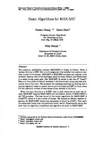
Three graphs. On the left, a tree with treewidth 1. On the right, a clique with treewidth 4. The graph in the middle has treewidth 2.
2.1
2
A sequence of graphs produced by eliminating vertices with the vertex elimination order π = (B,C,E,A,D). Each graph is labeled with the degree of the next vertex to be eliminated. The width of π is the maximum degree of any vertex when it is eliminated, thus, width(π) = max(3, 3, 2, 1, 0) = 3. . . . . . . . . . . . . . . .
2.2
9
A sequence of graphs produced by eliminating vertices from the same original graph as in Figure 2.1. The elimination order used in this case, πopt = (A,B,C,D,E), is optimal. Let G be the leftmost graph, treewidth(G) = width(πopt ) = max(2, 2, 2, 1, 0) = 2. Notice that there is more than one optimal elimination order. . .
9
2.3
A graph we seek to find the treewidth of. . . . . . . . . . . . . . .
13
2.4
The vertex elimination order search space for the graph given in Figure 2.3. Each state is labeled by the unordered set of vertices that have been eliminated from the graph at that point. An edge represents the operation of eliminating a vertex from the remaining graph, and each edge is labeled with the degree of the vertex being eliminated. Notice that the structure of this search space is a subset lattice. . . . . . . . . . . . . . . . . . . . . . . . . . . . . .
viii
13
2.5
The tree expansion of the search space in Figure 2.4. Each node is labeled by the elimination order prefix that led to it. Notice the presence of duplicate nodes that correspond to a single state in Figure 2.4. For example, nodes ABC, ACB, BAC, BCA, CAB, and CBA all correspond to the state {A,B,C}. . . . . . . . . . . .
4.1
14
A graph for which we construct tree decompositions, k-tree embeddings, and triangulations.
. . . . . . . . . . . . . . . . . . . .
22
4.2
Three tree decompositions of the graph in Figure 4.1. . . . . . . .
22
4.3
Two chordal graphs that are triangulations of the graph in Figure 4.1. Both have maximum clique sizes equal to 4. The graph on the left is also a 3-tree. . . . . . . . . . . . . . . . . . . . . . .
6.1
22
The graph on the right is a subgraph of the graph on the left, derived by removing vertex A. Notice that the degree of the graph on the left is 2, whereas the degree of its subgraph is 3. . . . . . .
6.2
38
The graph on the right is a minor of the graph on the left, derived by contracting the edge between vertices A and B. Notice that the degree of the graph on the left is 2, whereas the degree of its minor is 4. . . . . . . . . . . . . . . . . . . . . . . . . . . . . . . . . . .
6.3
A counter-example that demonstrates that MMD+(min-d) and MMD+(least-c) are not consistent heuristics. . . . . . . . . . . . .
6.4
39
43
During a search for optimal elimination orders on this graph, it is possible that GRDC and AVDC would prune all optimal solutions. 48
ix
6.5
The first level of the elimination order search space for the graph in Figure 6.4. Each edge is labeled with the eliminated vertex and its degree. The nodes labeled ‘X’ cannot lead to optimal solutions. The remaining nodes do lead to optimal solutions, though GRDC and AVDC may prune all of their children. . . . . . . . . . . . . .
6.6
Graph that results from eliminating vertex A from the graph in Figure 6.4. Notice that vertices D and G are simplicial. . . . . . .
7.1
63
Sample graphs for which NaiveMaxBF reopens many nodes. Nodes are labeled with their heuristic values. . . . . . . . . . . . . . . .
7.6
56
Two paths in a search space that demonstrate when a closed node may be reopened. . . . . . . . . . . . . . . . . . . . . . . . . . . .
7.5
52
The nodes and paths referred to in the definition of order preservation. . . . . . . . . . . . . . . . . . . . . . . . . . . . . . . . . .
7.4
51
The graph structure of the elimination order search space for a finding the treewidth of a graph with 4 vertices. . . . . . . . . . .
7.3
48
The search space for finding the treewidth of a graph with four vertices when no duplicates are eliminated. . . . . . . . . . . . . .
7.2
48
70
A decision tree used to store an open list in Zhou and Hansen’s method for deriving intermediate graphs. The open list shown here corresponds to a run of the BFHT algorithm, and it includes all nodes at depth two of a search for the treewidth of a graph with four vertices. . . . . . . . . . . . . . . . . . . . . . . . . . . . . . .
7.7
85
Partial decision trees that generate subtrees on the fly. These two trees show what the decision tree in Figure 7.6 looks like at various points during traversal. . . . . . . . . . . . . . . . . . . . . . . . .
x
89
7.8
A sorted open list at depth two in a BFHT search for a graph with four vertices. The list includes all nodes at depth two in Figure 7.2. Nodes are sorted in reverse lexicographic order so that they are expanded in the same order as in previous examples. . .
7.9
91
Nodes expanded by each algorithm, averaged over sets of samesized random graphs. . . . . . . . . . . . . . . . . . . . . . . . . .
95
7.10 Running time of each algorithm, averaged over sets of same-sized random graphs. . . . . . . . . . . . . . . . . . . . . . . . . . . . .
96
7.11 Memory usage of each algorithm, averaged over sets of same-sized random graphs. . . . . . . . . . . . . . . . . . . . . . . . . . . . .
97
7.12 Running time of BestTW and BFHT with neighbor-based graph derivation on all random graphs that both algorithms solved. Each point corresponds to a graph. Contour lines show where algorithms are equivalent, labeled “1x,” and where BestTW is three-times faster than BFHT, labeled “3x.” . . . . . . . . . . . . . . . . . . .
99
7.13 Running time of BestTW and QuickBB on all random graphs that both algorithms solved. Each point corresponds to a graph. Contour lines show where algorithms are equivalent, and where BestTW is fifteen-times faster than BFHT. . . . . . . . . . . . . . 100 7.14 Running time of both versions of BFHT on each random graph that both algorithms solved. The solid line shows where the neighborbased graph derivation technique is 1.425-times faster.
. . . . . . 101
7.15 Memory usage of BestTW and BFHT on each random graph that both algorithms solved. Contour lines show where BFHT uses from 0.25- to 0.6-times the amount of memory that BestTW does. 102
xi
8.1
Part of a graph with at least five vertices: v, w, x, y, and z. The circle in the middle indicates the rest of the graph. The only edges between the shown vertices are (v, z) and (w, y). Each of the shown vertices may be adjacent to zero, one, or many other vertices in the graph. . . . . . . . . . . . . . . . . . . . . . . . . . . . . . . . 125
8.2
An example of how the nogood (ng) data is updated and used to implement IVPR for the graph shown in Figure 8.1. Assume the nodes are generated left-to-right. Also, among vertices v, w, x, y, and z, the only edges are (w, y) and (v, z), as shown in Figure 8.1. 125
8.3
Two different orders of eliminating vertices A, B, and C from the graph on the left. . . . . . . . . . . . . . . . . . . . . . . . . . . . 127
8.4
Part of a IDTW search tree, where the first child of n was generated by eliminating vertex A. The search below that node completed without finding a solution with cost ≤ cutoff. The search then continues by eliminating vertices B, then C, then A from n. The question is: Is the resulting node m a duplicate of a node expanded previously? . . . . . . . . . . . . . . . . . . . . . . . . . . . . . . 127
8.5
A dependent vertex sequence s = (v1 , . . . , vr ) partitions the graph into three components: S, the set of vertices in s; S-ADJ, the set of vertices not in s but adjacent to some vertex in s; and REST, the set of vertices not in s and not adjacent to any vertices in s. . 131
8.6
Graphs resulting from vertex eliminations p = (A,G,B,C). When vertex C is eliminated and the node associated with graph G4 is generated, we will run FIND-VDVS on each of the preceding graphs to find any valid dependent vertex sequences.
xii
. . . . . . . . . . . 134
8.7
The subgraphs induced by vertices A, B, C, and G on the graphs in Figure 8.6. . . . . . . . . . . . . . . . . . . . . . . . . . . . . . 134
8.8
Partial depiction of the search paths discussed in the proof of Theorem 8.7. Edges are labeled with the eliminated vertex, and dashed edges indicate a series of eliminations not depicted. . . . . . . . . 143
8.9
Average nodes expanded by each algorithm on sets of random graphs. Only includes sets where all three algorithms were able to solve every graph without expanding any duplicate nodes. . . . 150
8.10 Average running time of each algorithm on sets of random graphs. Only includes sets where all three algorithms were able to solve every graph without expanding any duplicate nodes. . . . . . . . . 150 8.11 Nodes expanded by each algorithm, averaged over sets of samesized random graphs. . . . . . . . . . . . . . . . . . . . . . . . . . 153 8.12 Running time of each algorithm, averaged over sets of same-sized random graphs. . . . . . . . . . . . . . . . . . . . . . . . . . . . . 153 8.13 Memory usage of each algorithm, averaged over sets of same-sized random graphs. . . . . . . . . . . . . . . . . . . . . . . . . . . . . 154 8.14 Running time of IDTW+IVPR+DVPR and IDTW+TT+IVPR on all of the random graphs included in our experiments. Each point corresponds to a graph. The solid line shows where both algorithms have the same running time. . . . . . . . . . . . . . . . 155 8.15 Running time of IDTW+TT+IVPR on the most difficult instance from the 44-vertex set with various limitations on memory usage.
xiii
156
8.16 Running time, on all random graphs, of IDTW+IVPR+DVPR and DFBNB+IVPR+DVPR. The contour lines show where DFBNB is 1.5- and 3.5-times faster than IDTW. . . . . . . . . . . . . . . . . 158 8.17 Running time of DFBNB+IVPR+DVPR and BestTW on all random graphs that BestTW was able to solve. The contour lines show where DFBNB+IVPR+DVPR is 1.5 and three times faster than BestTW. . . . . . . . . . . . . . . . . . . . . . . . . . . . . . 160 8.18 Running time of DFBNB+IVPR+DVPR and BFHT on all random graphs that BFHT was able to solve. The contour lines show where DFBNB+IVPR+DVPR is two and eight times faster. . . . 160
xiv
List of Tables
7.1
Comparison of node expansions by NaiveMaxBF and MaxBF on pathological graphs. . . . . . . . . . . . . . . . . . . . . . . . . . .
7.2
71
Running time on benchmark graphs. ‘mem’ denotes algorithm required > 1800MB of memory and did not complete. . . . . . . . 103
8.1
Number of random graphs solved by BestTW and BFHT from the 50 in each parameter set. . . . . . . . . . . . . . . . . . . . . . . . 159
8.2
Running time on select benchmark graphs. The column labeled V gives the number of vertices in a graph, and VR gives the number of vertices in the a graph after an initial application of the graph reduction rules. DFBNB refers to DFBNB+IVPR+DVPR, and IDTW refers to IDTW+IVPR+DVPR. ‘mem’ denotes the algorithm required > 1800MB of memory and did not complete. ‘*’ denotes that a graph was made up of multiple connected components, and the reported data corresponds to the component with the greatest treewidth. . . . . . . . . . . . . . . . . . . . . . . . . 162
xv
List of Algorithms 7.1
BF*(Start node s): returns an optimal solution path, or nothing if no solution exists. . . . . . . . . . . . . . . . . . . . . . . . . . . .
7.2
MaxBF(Start node s): returns an optimal solution path, or nothing if no solution exists. . . . . . . . . . . . . . . . . . . . . . . . . . .
7.3
80
BFHT AUX(Graph G, cutoff ): returns an elimination order for G with width ≤ cutoff is one exists, otherwise returns (). . . . . . .
8.1
73
BFHT(Graph G): returns a tuple horder, widthi, where order is an optimal elimination order of G and width is the treewidth. . . . .
7.5
69
BestTW(Graph G): returns a tuple horder , widthi, where order is an optimal elimination order for G and width is the treewidth. . .
7.4
54
80
IDTW(Graph G): returns a tuple horder, widthi, where order is an optimal elimination order of G and width is the treewidth. . . . . 109
8.2
IDTW AUX(Graph G, cutoff ): returns an elimination order for G with width ≤ cutoff if one exists, otherwise returns (). . . . . . . . 109
8.3
DFBNB(Graph G, lb, ub): returns a tuple horder, widthi; if the treewidth of G is ≥ lb and < ub, then order = an optimal elimination order and width = the treewidth of G; if the treewidth is < lb then order = some elimination order with width ≤ lb and width = lb; if the treewidth is ≥ ub then order = () and width = ub. 110
8.4
FIND-VDVS(Graph G, Order p = (v1 , . . . , vr ) of vertices in G): returns a valid dependent vertex sequence in G made up of vertices in p, beginning with v1 and ending in vr , if such a sequence exists. Otherwise return (). . . . . . . . . . . . . . . . . . . . . . . . . . 133
xvi
Acknowledgments Thank you to Rich Korf, without whom this dissertation and the research it represents would not have been possible. Rich’s clear and engaging teaching style originally attracted me to the area of heuristic search algorithms. He showed me that solving the most important problems can be as fun as some of the most trivial, and that what we learn while tinkering with toys can lead to insights that push the limits of what is possible. As an advisor, Rich taught me that hard work, individual initiative, rational thinking, and high standards are the keys to successful research. He has served as a role model in how to do highquality research, write clear papers, and give engaging presentations. He has made himself exceedingly available to read rough drafts, listen to practice talks, and help out when I have thought myself into a corner. For all of his time and dedication I am eternally grateful. Thank you also to Adnan Darwiche. It was in his course on Reasoning with Partial Beliefs that I first encountered the concept of treewidth and elimination orders. He convinced me of the importance of this problem and provided motivation for much of the research presented in this dissertation. Also, thanks to Adam Meyerson and Lei He for devoting time and thought to serving on my committee, evaluating my work, and giving me feedback. Thanks to Vibhav Gogate and Rong Zhou for helpful discussions related to their respective work on treewidth. Also, thanks to Vibhav for providing me with the source code for his QuickBB algorithm, which helped kick-start my research. I am indebted to Alex Fukunaga. As my senpai, he has frequently served as a second advisor. Alex has taught me much about finding interesting research problems and how to be tenacious in making progress on them. He has shown
xvii
me how to put both my successes and failures in a wider context. I also owe thanks to many of my fellow students. Especially Arthur Choi, for providing me with endless breaks that were often more productive than the work I was breaking from. To my fellow students working on search and the like: Teresa Breyer, Eric Huang, Jim Clune, Seph Barker, Ethan Schreiber, and Cesar Romero. Thanks for many helpful discussions and welcome distractions. Thanks to Verra Morgan for invaluable help navigating the bureaucracy of graduate school, and more so for making the department feel like a family. Thanks to Deepak Khosla for showing me another side of research at HRL. This dissertation is the culmination of a long education.
So, thanks to
some of the best teachers I had along the way: Dave Mathews, Ron Palmer, Sheila Fitzgerald, Rob St. Clair, Bill Germann, Tom Halloran, Marty Teigen, Carmichael Peters, Gerald Alexanderson, Ed Schaefer, and the rest of the Santa Clara University Math/CS Department. Thanks to my friends and family, without whom none of this would matter anyway. My parents Paul and Deb Dow. My brothers Bryan and Scott Dow. My grandparents Angelo and Eda Grassi. Your encouragement and support have been invaluable. Any pride I feel for this accomplishment is a reflection of what I hope to inspire in you. Also, thank you to my in-laws. Haripal and Harwinder Arora. Amar Arora and Danielle Aretz. A good amount of the work reflected in this dissertation was done in the office in your home, where I was sustained by homemade food and regular deliveries of hot tea. Finally, thank you to my wife Anjuli for the emotional, financial, and sometimes physical support you have lent me throughout this process. I cannot imagine having completed this task without your love and devotion. Thank you.
xviii
Vita
1979
Born, Kansas City, Missouri, USA
2002
B.S. (Computer Science), Santa Clara University
2004–2008
Research Intern, HRL Laboratories, LLC, Malibu, California
2005
M.S. (Computer Science), University of California, Los Angeles
2008
Fellow, National Science Foundation East Asia and Pacific Summer Institutes, Tokyo Institute of Technology, Tokyo, Japan
Publications
P. Alex Dow and Richard E. Korf. Best-first search for treewidth. In Proceedings of the 22nd AAAI Conference on Artificial Intelligence (AAAI-07), pages 1146– 1151, Vancouver, British Columbia, Canada, July 2007. AAAI Press.
P. Alex Dow and Richard E. Korf. Best-first search with a maximum edge cost function. In Proc. of the 10th International Symposium on Artificial Intelligence and Mathematics (ISAIM-08), Fort Lauderdale, Florida, USA, January 2008.
P. Alex Dow and Richard E. Korf. Duplicate avoidance in depth-first search with applications to treewidth. In Proc. of the 21st International Joint Conference on Artificial Intelligence (IJCAI-09), Pasadena, California, USA, July 2009.
xix
Abstract of the Dissertation
Search Algorithms for Exact Treewidth by
P. Alex Dow Doctor of Philosophy in Computer Science University of California, Los Angeles, 2010 Professor Richard E. Korf , Chair
Treewidth is a fundamental property of a graph that has implications for many hard graph theoretic problems. NP-hard problems such as graph coloring and Hamiltonian circuit can be solved in polynomial time if the treewidth of the input graph is bounded by a constant. Given a graph, we can find its treewidth, or an approximation of its treewidth, by examining one of a number of compilations of the graph including vertex elimination orders, tree decompositions, and graph triangulations. Each of these compilations has a parameter referred to as its width, and they are optimal if their width is minimal. This minimal width is what we call the treewidth of a graph. Areas of artificial intelligence research, including Bayesian networks, constraint programming, and knowledge representation and reasoning, are based on queries and operations that are frequently infeasible without optimal or near-optimal vertex elimination orders, tree-decompositions, or other similar compilations. This dissertation deals with techniques for constructing these compilations optimally and finding the exact treewidth of a graph. Finding exact treewidth and optimal elimination orders are NP-complete problems. This dissertation describes techniques that use a heuristic search approach to prune large parts of the treewidth solution space and find exact
xx
treewidth quickly on hard benchmark instances. The final result is a state-of-theart algorithm for finding optimal elimination orders and exact treewidth. The algorithm uses a depth-first search with a variety of pruning techniques. The performance of previous depth-first algorithms suffered due to a large number of duplicate node expansions. Common methods for detecting and eliminating duplicate nodes rely on a large amount of memory. The techniques introduced here eliminate all duplicate nodes while only requiring a small amount of memory in practice. Furthermore, the search space used to find exact treewidth is unusual in that the cost of a solution path is the maximum edge cost on the path. There has been little previous research on problems such as this in the heuristic search literature. This dissertation includes several novel results related to heuristic search with a maximum edge cost function.
xxi
CHAPTER 1 Introduction Graphs are simple structures that permeate our lives. From roads between cities to the networks of relationships that fill our social lives, much of the world can be represented by graphs. At its most primitive, a graph is a collection of vertices connected by edges. We can take some information about the world, say a road map, and represent it as a graph. The cities, points of interest, and intersections become vertices, and the roads between them become edges. Figure 1.1 shows three examples of graphs. Once we have a graph, we can measure it and ask questions about it. How many vertices does it have? How long is the shortest path between two specific vertices? What is the smallest number of edges incident to any vertex? Can we traverse the graph, visiting every vertex exactly once, and return to where we started? The answers to these questions and many more represent properties that can be used to compare and categorize graphs. This dissertation is focused on one property in particular. While this property is not as intuitive as some of those just mentioned, it reveals an underlying structure in a graph that can be used to answer much more complicated questions.
1.1
Treewidth
The graph property that this dissertation is focused on is known as the treewidth of a graph. Informally, we can think of treewidth as a number that gauges how
1
Figure 1.1: Three graphs. On the left, a tree with treewidth 1. On the right, a clique with treewidth 4. The graph in the middle has treewidth 2. close a graph is to being a tree. A tree is a special kind of graph where there are no cycles, therefore, in a tree, there is exactly one path between any two vertices. The left-most graph in Figure 1.1 is an example of a tree. Most graphs are not trees; for example, see the other two graphs in Figure 1.1. We can think of treewidth as characterizing a spectrum of graphs, where we have the most tree-like graphs at one end and the least tree-like graphs at the other end. The most tree-like graphs are trees themselves and, therefore, have a treewidth of one. On the other end of the spectrum are complete graphs or cliques. A clique is a graph where every vertex is adjacent to every other vertex; for example, see the right-most graph in Figure 1.1. A clique with n vertices is the least tree-like type of graph, and it has a treewidth of n − 1. Every other graph lies somewhere between these extremes. Treewidth as a measure of “tree-likeness” is based on several specific ways of representing a graph. These include so-called k-tree embeddings, graph triangulations, tree decompositions, and vertex elimination orders, among others. Later in the dissertation (Chapters 2 and 4) we describe these structures in detail and formally define treewidth in the process. For now, it suffices to say that these data structures represent the underlying tree structure of a graph, and the treewidth is a measure of the size of that structure.
2
Understanding the tree structure underlying a graph can play a pivotal role in answering complicated questions about a graph. For example, consider the Hamiltonian Circuit problem (GT37 in Garey and Johnson [1979]). Given a graph, this problem asks whether it is possible to traverse the graph, visiting every vertex exactly once, and ending up back where we started. Hamiltonian Circuit is an NP-complete problem, therefore it is unlikely that we can devise an efficient method for solving it on arbitrary graphs. That being said, if we know that the treewidth of a specific graph or class of graphs is small and we have one of the associated data structures mentioned above, we can use that information to develop a fast and efficient algorithm. In addition to Hamiltonian Circuit, there are a large number of graph problems that are easy to solve for graphs with small, bounded treewidth. We go into this more in Chapter 3. In addition to well-known graph properties, such as Hamiltonian Circuit, treewidth also plays a role in a large and growing subfield of artificial intelligence research known as graphical models (see Pearl [1988], Dechter [2003], and Darwiche [2009]). The basic idea of graphical models research is to take some information about the world and represent it as a graph. Then a series of queries and operations are executed on the graph in order to answer fundamental questions about the represented data. An example of graphical models research is Bayesian networks, where the graph represents correlations among random variables. Applications of Bayesian networks include computational biology, medical diagnosis, information retrieval, and many other areas that involve probabilistic reasoning. Fundamental queries include finding the probability of some particular set of occurrences, or computing the most likely explanation for some outcome. Many of the most prevalent algorithms for answering these queries utilize an estimate of the graph’s underlying tree structure (i.e., the data structures mentioned earlier), and their complexity is closely related to the graph’s treewidth.
3
1.2
Solving Hard Problems with Heuristic Search
While the treewidth of some classes of highly structured graphs can be found easily [Bodlaender, 2005], determining the treewidth of an arbitrary graph is NP-complete [Arnborg et al., 1987]. A problem being NP-complete means that it is very likely that the only way to find exact solutions to arbitrary instances of this problem is an algorithm that runs in time exponential in the size of the instance. That means that small increases in the size of the problem will result in very large increases in the amount of time required to solve it. Therefore, even if you build a computer that is fast enough to solve a problem of size n, you will still be unlikely to solve problems of size n + 1 or n + 2. Many of the most interesting combinatorial problems that arise in the real world are NP-complete, therefore, though they may be technically “intractable,” people strive to solve them every day. When faced with NP-complete optimization problems, there are several dominant approaches that computer scientists take to dealing with them. While NPcompleteness implies that any algorithm likely requires exponential time in the worst case, it may be that some problem instances can be solved much faster. By restricting the input to problem instances with a specific structure, a polynomialtime algorithm may be possible. This research track has been thoroughly explored for the treewidth problem, and we review it in Chapter 4. Unfortunately, the graphs that occur in real-world instances of the treewidth problem rarely adhere to any structure sufficiently restrictive to make fast, polynomial-time algorithms widely applicable. Since the treewidth instances that arise in practice tend to be difficult to solve, another approach to dealing with them is called for. Perhaps the most prevalent approach to dealing with NP-completeness is approximation algorithms. While
4
it may take exponential time to find exact solutions to NP-complete problems, it may be possible that in polynomial time we can find solutions that are almost optimal. The field of approximation algorithms is focused on finding tractable algorithms that give solutions that are provably within some factor of an optimal solution. Approximation algorithms are used for a wide variety of real-world problems. They provide algorithms that scale well, while giving some guarantee on the quality of the solutions they return. Nevertheless, there are some problems where approximate solutions are not sufficient. Perhaps the available approximations are of poor quality, or it may be that suboptimal solutions of any degree are not acceptable. There has been a significant amount of research into approximation algorithms for treewidth, which we review in Chapter 4. While many of these algorithms are theoretically very interesting, they are less useful in practice. The solutions found by these algorithms tend to be of an unacceptably poor quality, and it is still unknown if it is possible to approximate treewidth within a constant factor in polynomial time. For a problem where approximation algorithms give poor solutions, or where problem instances are sufficiently diverse as to elude restrictive, exact, polynomialtime algorithms, a third approach is required. NP-completeness likely mandates that exact solutions to arbitrary problem instances will require exponential algorithms that essentially iterate through almost all possible solutions. Faced with this reality, the field of heuristic search research embraces this challenge head-on. For optimization problems, like treewidth, heuristic search reduces the problem to one of an agent searching for optimal paths in an abstract problem space. As the agent traverses the exponentially large space, it constructs partial solutions to the problem. Since the problem space includes all possible solutions to the prob-
5
lem, in the worst case the agent faces the task of an exponentially large search. In practice however, the agent can use a variety of tools and problem-specific knowledge to rule out large portions of this space.
1.3
Overview
The goal of my research and the focus of this dissertation is to apply heuristic search techniques to the problem of finding the exact treewidth of graphs of realworld interest. In the next chapter, we formally define treewidth and the concept of optimal vertex elimination orders. Additionally, we describe the problem space that is the focus of our search algorithms. In Chapter 3 we discuss in more detail the applications of treewidth and vertex elimination orders, and the role they play in making hard problems easier. In Chapter 4 we go into more detail on the mathematical foundations of treewidth, and we discuss previous efforts to deal with the intractability of treewidth. Chapter 5 details prior art on which my research builds. This includes various approaches to developing exact algorithms for arbitrary instances of treewidth. Chapter 6 describes a set of tools that we utilize in our searches, but which were developed by previous researchers. The primary contributions of this dissertation are detailed in Chapters 7 and 8. Chapter 7 discusses my work applying best-first search techniques to the treewidth problem. The efforts described in this chapter result in a significant advance in the state of the art. They are based on an observation about the topology of the underlying search space that allows for a much more efficient search than previous methods. Chapter 8 deals with my research on applying depth-first search techniques to the treewidth problem. As we will see, my work was not the first to use depth-
6
first search in this problem space, but by utilizing what was learned in the course of developing best-first search algorithms, I was able to develop what is currently the state-of-the-art algorithm for finding exact treewidth. The techniques that go into this algorithm make up what are likely the most significant contributions of this dissertation. With a technique I refer to as duplicate avoidance, I am able to turn depth-first search for treewidth from a tree search algorithm that does a large amount of duplicate search into a graph search algorithm that does no duplicate search. This results in a smaller and therefore faster search compared to previous algorithms. Furthermore, this is accomplished with a very small memory requirement in practice. While previous search algorithms for treewidth suffered due to a large amount of duplicate search or large memory requirements, the techniques described in Chapter 8 avoid both of these issues. Nevertheless, various computational bottlenecks and room for improvement remain, and we discuss these as well. In addition to describing various algorithms and tools that allow for fast exact treewidth solutions, throughout the dissertation we discuss novel issues that arise related to the field of heuristic search in general. As we will see shortly, the problem space that our algorithms search to find treewidth is unusual in that it uses a maximum edge cost function. While the existence of such a cost function has been mentioned in various places in the literature, to my knowledge no real problems that utilize it have been previously proposed. In the course of developing my treewidth algorithms, I have shown several novel results related to the behavior of common search algorithms on problems with such a cost function.
7
CHAPTER 2 Treewidth Definition and Search Space As mentioned in the previous chapter, the treewidth of a graph is a scalar value that indicates how close the graph is to being a tree. Associated with the treewidth is a variety of data structures that represent a graph’s underlying tree structure. These include k-tree embeddings, graph triangulations, and tree decompositions; all of which we will discuss in more detail in Chapter 4. In the mean time we will focus on vertex elimination orders, which are closely related to these other structures. Using vertex elimination orders we provide a formal definition of treewidth and describe a problem space that is the foundation of our search algorithms.
2.1
Treewidth and Optimal Vertex Elimination Orders
We formally define treewidth in terms of vertex elimination orders. The notion of finding optimal vertex elimination orders is based on Bertel`e and Brioschi’s [1972] work on nonserial dynamic programming, and plays a role in a variety of algorithms in graphical models. This includes, among others, the bucket elimination [Dechter, 1996] approach to constraint programming and inference in Bayesian networks. We begin with a series of definitions. First of all, we define the operation of eliminating a vertex from a graph as the process of adding an edge between
8
A
A
B
C
D
E
Deg(B) = 3
D
A
C
C
E
D
Deg(C) = 3
A
C
E
Deg(E) = 2
D
D
Deg(A) = 1 Deg(D) = 0
Figure 2.1: A sequence of graphs produced by eliminating vertices with the vertex elimination order π = (B,C,E,A,D). Each graph is labeled with the degree of the next vertex to be eliminated. The width of π is the maximum degree of any vertex when it is eliminated, thus, width(π) = max(3, 3, 2, 1, 0) = 3.
A
B
C
B
D
E
D
Deg(A) = 2
A
C
E
Deg(B) = 2
A
D
C
E
Deg(C) = 2
D
A
E
Deg(D) = 1
E Deg(E) = 0
Figure 2.2: A sequence of graphs produced by eliminating vertices from the same original graph as in Figure 2.1. The elimination order used in this case, πopt = (A,B,C,D,E), is optimal. Let G be the left-most graph, treewidth(G) = width(πopt ) = max(2, 2, 2, 1, 0) = 2. Notice that there is more than one optimal elimination order.
9
every pair of a vertex’s neighbors that are not already adjacent, then removing the vertex and all edges incident to it. In Figure 2.1, the second graph from the left is the result of eliminating vertex B from the first graph. Clearly, eliminating a vertex is different from merely removing the vertex and its incident edges, namely because its former neighborhood now induces a clique. A vertex elimination order is a total order over the vertices in a graph, which tells us what order to eliminate the vertices in. By eliminating the vertices in a given order, we produce a sequence of graphs. For example, Figure 2.1 shows the sequence of graphs that result from applying the elimination order π = (B,C,E,A,D) to the left-most graph in the figure. We can measure an elimination order by its width. The width of an elimination order is defined as the maximum degree of any vertex when it is eliminated from the graph. In Figure 2.1, each graph is labeled by the degree of the vertex that is next to be eliminated in order π. The width of π is the maximum of these values, i.e. width(π) = max(3, 3, 2, 1, 0) = 3. Finally, the treewidth of a graph is the minimum width over all possible elimination orders, and any order whose width is the treewidth is an optimal vertex elimination order. Figure 2.2 shows the sequence of graphs that results from an optimal elimination order on the same original graph as Figure 2.1. The treewidth of this graph is 2.
2.2
Heuristic Search for Treewidth
In order to apply heuristic search methods to finding exact treewidth, we cast the problem as one of single-agent pathfinding. In this abstraction, we seek a path from a start state to a goal state through some search space. Such a path
10
corresponds to a solution to our problem, and, therefore, we seek a path that gives us an optimal solution. To make treewidth into a pathfinding problem, we must first define the search space. Vertex elimination orders suggest a natural search space. At the start state, our search begins with an empty elimination order. We can then transition from one state to another by adding a vertex to the elimination order. A goal state is reached once every vertex in the graph has been eliminated. Since one vertex is added to the elimination order on each edge transition in the search space, the path taken from the start to the goal corresponds to an elimination order. Notice that, as the search progresses, the original problem is divided into subproblems that we seek solutions to. Initially, we seek an optimal vertex elimination order for the original graph. Then, when we add a vertex to the elimination order, we eliminate that vertex from the graph. At the new state in the search space, we now seek an elimination order for the new graph that results from the last elimination. In this way, every state in our search space corresponds to a graph that is derived from the original graph by following the sequence of eliminations on the path taken from the start state. Our goal is to find a vertex elimination order with minimal width. Once we find a complete solution path from the start to the goal, we can evaluate it to determine the width of the corresponding elimination order. Recall that the width of an elimination order is the maximum degree of any vertex when it is eliminated from the graph. Since an edge transition in our search space corresponds to eliminating a vertex from the graph, we can label each edge with the degree of the eliminated vertex. That is the cost of an edge. Once a complete solution path is found, we evaluate it with a cost function, where the cost of a path is the maximum edge cost on the path. Clearly, this is equal to the width
11
of the elimination order. In terms of our search, the treewidth problem is now to find a minimal-cost solution path in the vertex elimination order search space. We should point out that this maximum edge cost function is unusual. Most problems in the search literature use an additive cost function, where the cost of a path is the sum of the edge costs. Examples of additive-cost problems include sliding tile puzzles and road navigation. The fact that our search space uses a maximum edge cost function will have a variety of implications for the search algorithms we employ. A final important detail about the elimination order search space has to do with multiple paths to the same state. In what they called the Invariance Theorem, Bertel`e and Brioschi [1972] showed the following: eliminating a given set of vertices from a graph in any order produces the same graph. This means that every permutation of some set of vertex eliminations produces a path that leads to the same state in the elimination order search space. For an example of what this search space looks like for the graph in Figure 2.3, see Figure 2.4. Notice that we label each state with the unordered set of vertices eliminated in order to reach it. Each path to a state corresponds to a different permutation of those eliminated vertices. For example, notice that eliminating B then C leads to the same state, {B,C}, as eliminating C then B. Although they lead to the same state, these two paths do not incur the same cost. BC has cost max(2, 2) = 2, and CB has cost max(3, 2) = 3. Nevertheless, regardless of the path taken to a state, the rest of the search space below it is the same. In our discussion of searching for treewidth and optimal elimination orders, we refer to two different graphs. One is the graph instance for which we seek the treewidth and an optimal elimination order. The other is the search graph. Figure 2.3 is an example of the first, and Figure 2.4 is an example of the second.
12
A
B
C
D
Figure 2.3: A graph we seek to find the treewidth of.
{} 2 {A}
1 2
{A,B}
1 1
1
1
{A,C} 1
{A,B,C} 0
1
2 {B}
2
1
2
{A,D} 1 1
3
1
{C}
2
2
2
1
{B,C} 1
{A,B,D}
{A,C,D}
0
0
{D}
2 2
1
{B,D}
1 1
{C,D}
1
{B,C,D} 0
{A,B,C,D} Figure 2.4: The vertex elimination order search space for the graph given in Figure 2.3. Each state is labeled by the unordered set of vertices that have been eliminated from the graph at that point. An edge represents the operation of eliminating a vertex from the remaining graph, and each edge is labeled with the degree of the vertex being eliminated. Notice that the structure of this search space is a subset lattice.
13
2
2
A
1
1
1
AC
1
AD
1 1
1 1
1
B
2
AB
3
2
BA
1 1
C
1
BC
1 1
2
BD
1 1
2
CA
1 1
DBC
DCA
DCB
0
0
0
0
0
0
0
DBCA
DCAB
DCBA
BDCA
0
DBAC
BDAC
DBA
BCDA
0
DACB
BCAD
DAC
BADC
0
DABC
BACD
DAB
ADCB
0
CDBA
ADBC
CDB
ACDB
0
CDAB
ACBD
CDA
BDA 0
ABDC
0
CBDA
BCD 0
1
CBD
BCA 0
1 1
CBAD
BAD 0
1 1
DC
CBA
BAC 0
1 1
DB
CADB
ADC 0
1 1
DA
2
CAD
ADB 0
1 1
CD
2
CABD
ACD 0
CB
2
CAB
ACB 0
2
BDC
ABD 0
ABCD
ABC 0
D
Figure 2.5: The tree expansion of the search space in Figure 2.4. Each node is labeled by the elimination order prefix that led to it. Notice the presence of duplicate nodes that correspond to a single state in Figure 2.4. For example, nodes ABC, ACB, BAC, BCA, CAB, and CBA all correspond to the state {A,B,C}.
14
To differentiate between them we use the following terminology. The points in a graph instance we seek the treewidth of will be referred to as vertices, while the points in the search graph will be referred to as states or nodes. When using the word “graph,” the context will make it clear which is being referred to. Notice that a graph instance is always undirected, while the search graph is directed. Also, only the search graph has values associated with its edges. A fundamental concept in heuristic search is a search node. A search node is characterized by a particular path from the root to a state. If a search graph is a tree, then there is exactly one node for each state in the problem space. If a search space does not have a tree structure, then there is more than one path to at least some states in the problem space. Thus, each unique path to the same state results in a different node. Two nodes that represent distinct paths to the same state are referred to as duplicate nodes. A tree expansion of a search graph is the tree that results from representing each node as a distinct vertex. The tree expansion of the search space in Figure 2.4 is shown in Figure 2.5. Notice that, for a graph with n vertices, the elimination order search graph has 2n states, whereas the tree expansion has O(n!) nodes. The distinction between these representations of the search space will have a significant impact on the algorithms we employ to search it.
15
CHAPTER 3 Applications of Treewidth 3.1
Parametrized Complexity
Treewidth is well-known and well-studied primarily because of the role it plays in parameterized complexity. Parameterized complexity involves analyzing the complexity of problems in terms of multiple input parameters. While a problem may require exponential time when only the size of the input is considered, it may have an algorithm that is actually polynomial in the input size and exponential in some other parameter. For example, graph coloring is an NP-hard problem, therefore, assuming P 6= NP, solving it generally requires time exponential in the size of the input. In fact, there exists an algorithm for graph coloring that is linear in the size of the graph and exponential in the treewidth of the graph [Arnborg and Proskurowski, 1989]. In general, treewidth is only bounded by the size of the graph, therefore that algorithm still requires exponential time on arbitrary graphs. If analysis is restricted to graphs with treewidth bounded by a constant, then graph coloring can be solved in time linear in the size of the graph. One of the primary uses of parameterized complexity is to show that some hard problems become tractable when some parameter of the input is bounded by a constant. Treewidth is a particularly interesting graph parameter, because bounding it makes many hard problems tractable. Courcelle [1990a, 1990b] demonstrated that determining if a graph satisfies
16
any property that can be written in monadic second-order logic is tractable if the input graph has constant bounded treewidth. Courcelle [1990a] described monadic second-order logic (MSOL) as an extension of first-order logic and a restriction of second-order logic. A formula of MSOL can include variables that correspond to vertices, edges, sets of vertices, and sets of edges. It can include set membership relations and quantification over the variables. There are many NP-complete problems that are expressible in MSOL, including k-Colorability and Hamiltonian Circuit. Thus, on graphs of constant bounded treewidth, these problems become tractable.
3.2
Graphical Models
A significant amount of recent artificial intelligence research relates to so-called graphical models, including probabilistic reasoning, constraint satisfaction, and knowledge representation and reasoning. This research typically uses a graph to represent some information about the world. Various queries and operations are then carried out on the graph. Many of these queries are generally intractable, but become tractable if the graph has constant bounded treewidth. For example, the predominant algorithms for exact inference on Bayesian networks, including bucket elimination [Dechter, 1996], jointree [Lauritzen and Spiegelhalter, 1988], and recursive conditioning [Darwiche, 2001], have polynomial time complexity if the network’s treewidth is bounded by a constant. Other examples include techniques for constraint satisfaction, including backtracking with tree decompositions [J´egou and Terrioux, 2003, de Givry et al., 2006, J´egou et al., 2007] and jointree clustering [Dechter and Pearl, 1989]. In the area of knowledge representation and reasoning, several intractable reasoning methods such as abduction, closed world reasoning, circumspection, and disjunctive logic programming be-
17
come tractable on a graph with constant bounded treewidth [Gottlob et al., 2006, Gottlob et al., 2007]. While a constant bound on the treewidth of the graph makes the above mentioned problems tractable, in order for the corresponding algorithms to run in polynomial time, more information is required. These algorithms take, as additional input, a structured compilation of the graph that is characterized by its width. The compilation is used by the algorithms to direct their operations, and it is the width of the compilation that determines an effective bound on the treewidth of the input graph. For example, take the bucket elimination algorithm for inference on a Bayesian network. The algorithm requires as input, not only the network and a query, but also an elimination order over the variables in the network. The time complexity of bucket elimination is exponential in the width of the provided order. If the order is optimal, then its width is the treewidth of the network, and the algorithm will run as efficiently as possible. Since the width of the order is the exponent of the algorithm’s time complexity, even a slightly suboptimal order can significantly increase the running time of the algorithm. Some of the algorithms listed above require other compilations of the input graph besides an elimination order. These other compilations, including graph triangulations, tree decompositions or jointrees, dtrees, and k-tree embeddings, can also be measured in terms of their width. We discuss these compilations in more detail in the next chapter. Algorithms that require these other compilations have running times that, like the bucket elimination algorithm, are primarily determined by the width of the input compilation. Thus, although bounding the treewidth of the input graph by compiling it into one of these structures theoretically makes the problem tractable, if that bound is too large it may still be infeasible to solve real problem instances.
18
On a final note, our discussion of exact treewidth centers on finding optimal vertex elimination orders. Since some algorithms require other graph compilations, optimal elimination orders are only useful if they can be easily converted into jointrees, dtrees, etc. Fortunately there are polynomial-time conversions from elimination orders to various other graph compilations with the same or lesser width [Darwiche and Hopkins, 2001, Darwiche, 2009].
19
CHAPTER 4 Background In this chapter we discuss some of the background material related to treewidth. This includes alternate definitions of treewidth, other than the one we gave previously in terms of vertex elimination orders. All of these definitions of treewidth are equivalent, but the definitions that follow rely on different data structures for representing the underlying tree structure of a graph. We also discuss previous efforts to cope with the inherent intractability of the treewidth problem. In the introduction to this dissertation we described three common approaches to dealing with NP-completeness. One of these was exact exponential algorithms, which include the heuristic search techniques on which this dissertation is focused. In this chapter we discuss prior work on the other two approaches. These include polynomial-time algorithms for finding the exact treewidth of specific types of graphs, and approximation algorithms for arbitrary graphs.
4.1
Alternate Definitions of Treewidth
The term treewidth was coined by Robertson and Seymour [1986] in the second of their twenty-paper series on graph minors. Their definition of treewidth is in terms of a tree decomposition of a graph. As we mentioned earlier, treewidth can be defined in terms of several distinct concepts in graph theory. We discussed
20
vertex elimination orders, but early work on treewidth involved a variety of concepts that, at first glance, may not seem related. Here, we describe some of the most common ways of defining and understanding treewidth. Since Robertson and Seymour coined the term, we begin with their definition in terms of tree decompositions. We construct a tree decomposition for a specific graph with a set of procedures that turn the graph into a tree. The vertices of the graph are grouped into overlapping subsets, and each of these subsets are used to label a node in the tree. The subsets and the tree structure must be carefully constructed to adhere to a number of conditions. We will give the exact conditions shortly. For most graphs, there are many possible tree decompositions. Different tree decompositions for the same graph will often differ in the size of the vertex subsets. We refer to the size of the largest subset minus one as the width of a particular tree decomposition. The treewidth of a graph G is the minimum width among all possible tree decompositions of G. For an example of tree decompositions, Figure 4.2 shows three possible tree decompositions of the graph in Figure 4.1. The tree decomposition furthest to the left has minimal subset size, thus the treewidth of the graph is 3. The tree decomposition furthest to the right is the trivial decomposition, made up of a single subset containing all vertices in the graph. Now we give a formal definition of tree decomposition that includes the conditions on the subsets and tree structure. Definition 4.1. A tree decomposition of a graph G = (V, E) is a pair (X, T ), where X is set of subsets of V and T is a tree. Each node i in the tree T corresponds to exactly one of the subsets in X, denoted Xi ∈ X. The decomposition (X, T ) has the following properties:
21
A
B
C
E
D
F
G
Figure 4.1: A graph for which we construct tree decompositions, k-tree embeddings, and triangulations.
ABCD
ABCDF ABCDEFG
BCE
BDF
CDG
BCE
width = 3
CDG
width = 4
width = 6
Figure 4.2: Three tree decompositions of the graph in Figure 4.1.
A
E
B
A
D
G
E
B
D
C
C
F
F
G
Figure 4.3: Two chordal graphs that are triangulations of the graph in Figure 4.1. Both have maximum clique sizes equal to 4. The graph on the left is also a 3-tree.
22
•
S
i∈T
Xi = V ; every vertex in G is in at least one subset.
• If vertices v and w are adjacent in G, then there is at least one subset Xi that contains both v and w. • Given three nodes i, j, k in tree T , if j is on the path between i and k, then Xi ∩ Xk ⊆ Xj , i.e., every vertex in the subsets corresponding to both i and k must also be in the subset corresponding to j. Definition 4.2. The width of a tree decomposition D = (X, T ) is the size of the largest subset minus one, i.e., width(D) = maxXi ∈X |Xi | − 1 Arnborg, Corneil, and Proskurowski [1987], independent of Robertson and Seymour’s work, showed that finding the treewidth of a graph is NP-complete. While they did not use the term treewidth, their problem of finding minimal k-tree embeddings is equivalent. A k-tree can be defined recursively, as follows. Definition 4.3. A clique with k vertices is a k-tree. Also, a k-tree with n + 1 vertices can be constructed from a k-tree with n vertices by adding a new vertex that is adjacent to all vertices in some clique of size k. Definition 4.4. A partial k-tree is a subgraph of a k-tree. Clearly, every graph is a partial k-tree for a large enough k. The treewidth of a graph is equal to the smallest k such that the graph is a partial k-tree. This is the problem that Arnborg, Corneil, and Proskurowski demonstrated was NPcomplete (by reduction from the Minimum Cut Linear Arrangement problem, GT44 in Garey and Johnson [1979]). As mentioned previously, the treewidth of the graph in Figure 4.1 is 3, thus it is a partial 3-tree. On the left in Figure 4.3 we give a 3-tree for which that graph is a subgraph. We refer to the process of
23
showing the a graph is a subgraph of another graph as embedding one graph into another. Thus, a partial k-tree is a graph that can be embedded in a k-tree. A more general concept than k-trees is chordal graphs. Given a cycle in a graph, a chord is an edge between any two vertices that are not adjacent in the cycle. A graph is chordal, or triangulated, if every cycle of length greater than three has a chord. A k-tree is a type of chordal graph. Chordal graphs can be measured by the size of their largest clique. A k-tree is a chordal graph with maximum clique size k + 1. Given a graph that is not chordal, the process of adding edges to make it chordal is referred to as triangulating the graph. The treewidth of a graph is equal to the minimal maximum clique size minus one among all tringulations of the graph. The 3-tree on the left of Figure 4.3 is a minimal triangulation of the graph in Figure 4.1, with a maximum clique size of four. The graph on the right of Figure 4.3 is not a k-tree, but it is a minimal triangulation of the graph in Figure 4.1 with a maximum clique size of four. In addition to elimination orders, tree decompositions, k-tree embeddings, and graph triangulations, treewidth can be defined in terms of seperators, intersection graphs, and even “cops and robbers” games. This section is meant to introduce some of the commonly encountered data structures that define treewidth. The reader is not expected to achieve a deep understanding for these concepts or why they all define treewidth equivalently. For a more in-depth survey of the many equivalent definitions of treewidth see Bodlaender [1998]. While all of these notions give an equivalent definition of treewidth, the associated data structures are clearly very different. The applications discussed in Chapter 3 typically rely on one of these data structures. While the methods discussed in this dissertation are focused on finding optimal elimination orders, they are only useful to the various application areas if we can convert these orders
24
into these other data structures. Luckily, given an elimination order of width w, we can convert it into a tree decomposition with width no greater than w in polynomial-time. Likewise, using an elimination order, we can triangulate the graph into a chordal graph with maximum clique size no greater than w + 1, and we can embed the graph in a w-tree. The latter two processes are as simple as tracking all the edges added in the elimination process and adding them to the original graph (with a few more edges in the case of a k-tree). Converting an elimination order into a tree decomposition is slightly more complicated, though it can be done very quickly. Darwiche [2009], Chapter 9, describes the procedure in the context of inference algorithms for Bayesian networks. In the Bayesian network literature, a tree decomposition is referred to as a jointree. Likewise, Darwiche discusses another data structure called a dtree. Dtree’s are similar to another notion we did not discuss here, known as a branch decomposition of a graph. Dtree’s are also measured by their width, and an optimal dtree has width equal to a graph’s treewidth. As with jointrees, Darwiche shows how to build a dtree from an elimination order in polynomial time while preserving the width.
4.2
Graphs with Treewidth Computable in Polynomial Time
There has been much research on identifying specific types of graphs for which treewidth can be computed easily. Clearly, the graphs for which treewidth is easiest to compute are those with a known constant treewidth. For example, trees are known to have a treewidth of one. Other graphs, known as seriesparallel graphs, have a treewidth of two. Also, based on our discussion in the previous section, we know that k-trees have a treewidth of k. For more on graphs with bounded treewidth, see Bodlaender’s survey [1998].
25
There are other types of graphs that do not have constant treewidth, but for which the treewidth can be found in polynomial time. One example is a chordal or triangulated graph. To find the treewidth of a triangulated graph, we merely need to construct an elimination order where a vertex is added to the order only if its neighborhood induces a clique. There will always be at least one such vertex. Other graphs for which treewidth can be found in polynomial time include so-called permutation graphs, interval graphs, and circle graphs. For more on the complexity of treewidth on particular classes of graphs, including those just mentioned, see another of Bodlaender’s surveys [1993]. While there seems to be an extensive literature on these sorts of graphs, the graph classes on which treewidth can be found in polynomial time are rather restrictive. It is unrealistic to think that the graphs interesting to the application areas discussed in Chapter 3 would regularly fit into these classes. Thus, in order to develop a widely useful tool for finding treewidth, we cannot so restrict the sorts of graphs we are willing to consider.
4.3
Approximation Algorithms
As we saw in the last section, the classes of graphs for which treewidth can be found in polynomial time is rather restrictive. Therefore, in an effort to develop tractable algorithms for finding treewidth, there has been a significant amount of research into approximation algorithms. Some of the earliest polynomial-time approximation algorithms for treewidth were developed by Kloks [1994] and Bodlaender et al. [1995]. These algorithms gave a O(log n) approximation ratio, for a graph with n vertices. These algorithms return a tree decomposition of a graph, where the width of the returned decomposition is at most O(k log n) if the treewidth is k.
26
Amir [2001, 2008] and Bouchitt´e et al. [2004] developed polynomial-time algorithms with a O(log k) approximation ratio, where k is the graph’s treewidth. √ Feige, Hajiaghayi, and Lee [2005] improved upon this with a O( log k) approximation ratio. To the best of my knowledge, this is the state-of-the-art polynomialtime approximation algorithm for treewidth. It is currently unknown whether it is even possible to have an algorithm that runs in polynomial time and gives a constant-factor approximation for treewidth (see Amir [2008]). In light of this, there are a number of exponential-time algorithms that give constant-factor approximations. Amir [2001, 2008] reviews some of these algorithms and gives three new ones with approximation ratios of 4.5, 4.0 and 3.66. Each of these algorithms that gives a better approximation also has a larger exponential time complexity. Amir [2001, 2008] conducted a series of experiments to evaluate the effectiveness of these approximation algorithms. He compared the exponential-time algorithms with a simple heuristic method. The heuristic returns a solution very quickly, though it has no performance guarantee. The experiments showed that the solutions returned by the approximation algorithms were consistently much worse that the solution found by the heuristic method. While theoretically interesting, current approximation algorithms are unable to provide good enough solutions to result in a useful tool for finding treewidth. This is punctuated by the fact that even exponential-time algorithms could not compete with a simple heuristic. Therefore, we cannot expect acceptable performance from the polynomial-time approximation algorithms. In many of the application areas discussed in Chapter 3, even a small improvement in the width of an elimination order or tree decomposition can have a big impact. With that in mind, the remainder of this dissertation is focused on finding exact treewidth.
27
CHAPTER 5 Prior Art: Exact Algorithms Prior research on exact algorithms for computing treewidth can be grouped into three approaches. The first represents early work on finding treewidth where the focus was on the decision problem, i.e. for some k, is the treewidth ≤ k? By fixing k as a constant, these algorithms are able to claim polynomial time complexity. Unfortunately, in practice treewidth frequently grows with the size of the graph, therefore it is not realistic to consider k a constant. With this in mind, some recent research has focused on improving the asymptotic worst-case complexity of algorithms for finding exact treewidth. As we will see, these algorithms tend to work by iterating through sets of vertices that make up minimal separators or what is referred to as potential maximal cliques. While these algorithms strive to achieve the best asymptotic complexity bounds, there has been no work on evaluating them empirically. The third approach to finding exact treewidth focuses on empirical evaluation. These algorithms, including the search algorithms which are the subject of this dissertation, are meant to perform well in practice. They will employ short-cuts that do not affect the asymptotic worst-case analysis and yet, in practice, significantly improve performance. We now discuss these three approaches in order.
28
5.1
Fixed Parameter Algorithms
Early algorithms for finding exact treewidth were focused on achieving time complexity that is polynomial if the treewidth is bounded by a constant. Typically, these algorithms can find the treewidth, along with accompanying data structures such as k-tree embeddings or tree decompositions, very quickly for graphs with small treewidth. The first algorithm was proposed by Arnborg, Corneil, and Proskurowski [1987] in the same paper where they established that the problem is NP-complete. Their algorithm answers the treewidth decision problem by attempting to embed the graph in a k-tree, for some k. The algorithm has exponential time complexity in k, but if k is bounded by a constant, the complexity becomes polynomial. Arnborg, Corneil, and Proskurowski’s algorithm is based on finding separators of the graph. A separator is a set of vertices whose removal disconnects the graph into multiple connected components. The algorithm works by iterating through all sets of k vertices in order to find the separators of size k. The algorithm basically stores the components created by each separator, sorts them by size, and steps through the list, building a k-tree embedding in the process. The complexity is dominated by finding the separators. If there are n vertices in the � graph, then there are nk ∈ O(nk ) vertex sets of size k. Checking if each of these is a separator takes O(n2 ) time. Thus, the time complexity of this algorithm is O(nk+2 ), which, if k is a constant, is polynomial in n. Robertson and Seymour [1986] showed that the treewidth problem is fixed parameter tractable (FPT). A problem is FPT if there exists an algorithm with time complexity O(f (k) nc ), given problem size n, a constant c, a parameter k, and an arbitrary function f that depends only on k. Clearly, this differs from
29
Arnborg, Corneil, and Proskurowski’s algorithm which had time complexity of the form O(ng(k) ), for a polynomial function g. The reason for the distinction is that problems that are FPT can be considered tractable on instances where the parameter k is small, even if the problem size n is very large. Clearly, even with a moderately small k, if n is very large, then Arnborg, Corneil, and Proskurowski’s algorithm will be infeasible. For more on fixed parameter tractability, see Flum and Grohe’s textbook [2006]. While Robertson and Seymour showed that treewidth has a FPT algorithm, their proof was non-constructive. Based on several of their papers on graph minors, Bodlaender [1996] claims that they have proved the existence of a O(n2 ) algorithm, assuming treewidth is fixed, though they do not actually provide the algorithm. Since Robertson and Seymour [1986], a variety of fixed-parameter tractable algorithms for treewidth have been developed. Unfortunately, in practice, their performance is dominated by f (k), the typically large “constant” factor. The ultimate example of this is Bodlaender’s [1996] fixed-parameter linear algorithm, i.e., O(f (k) n). While theoretically interesting, the constant factor of this algorithm is so large that Bodlaender himself claims that it is “probably not practical, even for k = 4.”
5.2
Improving Worst-Case Performance
The algorithms from the previous section perform well, as long as the treewidth is small. In reality, many graphs have a treewidth that grows linearly with the number of vertices. More recent research has taken this into account and seeks algorithms where the worst-case asymptotic running time is as small as possi-
30
ble. Naturally, since treewidth is an NP-complete problem, these algorithms will almost certainly have an exponential running time. Generally, exponential running time is considered intractable, and little concern is given to how intractable. But, as I have tried to show in this dissertation, just because we cannot solve a problem easily, does not mean that we do not need to solve it anyway. If we must solve these hard problems, then we had best come up with the “least” intractable algorithms possible. Recent research has focused on these sort of exponential algorithms. As is frequently the case in algorithms research, the effectiveness of an algorithm is measured by it’s asymptotic worst-case complexity, i.e. big-oh notation. Naturally, big-oh notation suppresses constant factors, because they are irrelevant to a performance comparison of algorithms with different non-constant factors as the input size grows sufficiently. In the case of exponential algorithms, any sub-exponential factors in the complexity will be irrelevant if the input is large enough. Thus, exponential algorithms use a modified notation in order to express asymptotic behavior. Just as O suppresses constant factors, O∗ suppresses all sub-exponential factors. For example, cn2 2n ∈ O(n2 2n ) ∈ O∗ (2n ). For background on exponential algorithms research, see Woeginger’s survey [2003]. Research into algorithms with superior exponential asymptotic behavior for treewidth have predominantly involved finding all minimal separators and potential maximal cliques of a graph. The formal definitions of these concepts are not critical to our explanations here, therefore I will only give an intuitive explanation. Fomin and Villanger [2008] give formal definitions and a variety of results. A separator is a set of vertices that, if removed from the graph, will cause some pair of vertices to become disconnected. A minimal separator is a separator that separates some pair of vertices such that no proper subset of it also separates
31
those vertices. The best way to understand potential maximal cliques is in terms of chordal graphs or graph triangulations. Recall that treewidth can be defined in terms of graph triangulations, and that any particular triangulation is measured by the size of its largest clique. A potential maximum clique is any set of vertices such that that set of vertices induces a maximal clique in some minimal triangulation. There is a series of papers that utilize minimal separators and potential maximal cliques to find treewidth. Fomin, Kratsch, and Todinca [2004] developed an algorithm that finds treewidth and an optimal tree decomposition in time O(n3 (|ΠG | + |∆G |)), where ΠG is the set of potential maximal cliques and ∆G is the set of minimal separators. Naturally, there are an exponential number of minimal separators and potential maximal cliques in a graph, therefore this algorithm requires exponential time. Fomin and Villanger [2008] showed that the minimal separators of a graph could be listed in time O∗ (1.6181n ), and the potential maximal cliques could be listed in time O∗ (1.7549n ). Thus, using the mentioned algorithm the time required to list the potential maximal cliques dominates the time complexity, resulting in an algorithm for computing treewidth that runs in O∗ (1.7549n ) time. This algorithm requires that all of the separators and potential maximal cliques be stored, therefore the space requirement is also exponential. Bodlaender et al. [2006a] gave an algorithm that only requires a polynomial amount of space with running time O∗ (2.9512n ). Fomin and Villanger [2008] improved upon this to O∗ (2.6151n ) time.
32
5.3
Empirically Evaluated Algorithms
The algorithms described in the previous section represent the state-of-the-art techniques for finding exact treewidth in terms of asymptotic worst-case complexity. That being said, there has been no published effort to empirically evaluate these algorithms. Asymptotic analysis typically gives a good measure of how an algorithm will perform, assuming there are no large constant factors. With exponential algorithms, this may not be the case. Because the algorithms have an exponential time complexity, it may be infeasible for any algorithm to solve large enough problems to overcome any hidden polynomial factors. If we have little chance of solving a problem for large values of n, then the asymptotic behavior may not be relevant. For this reason, and because a worst-case analysis may not reflect performance in practice, empirical evaluation of treewidth algorithms is necessary in order to establish the state-of-the-art technique in terms of a useful tool for finding treewidth. A predecessor of the algorithms discussed in the previous section is Shoikhet and Geiger’s QuickTree algorithm [1997], which constructed optimal triangulations by iterating through the minimal separators of the graph. A significant difference between this and the previously discussed algorithms is that Shoikhet and Geiger utilized heuristics that allowed the algorithm to not consider certain separators. This did not affect the worst-case complexity of the algorithm, but it did produce an algorithm that was faster in practice than it would have been otherwise. Shoikhet and Geiger developed their algorithm with the goal of providing a useful tool for computing treewidth, and, therefore, they evaluated the algorithm empirically on various randomly generated graphs. The goal of my research, presented in this dissertation, is the same as that of Shoikhet and Geiger. The techniques developed here are meant to provide a
33
state-of-the-art tool for finding treewidth in practice. Typically the algorithms discussed in the previous section will have superior asymptotic worst-case complexity, but it is unlikely that these algorithms will be competitive on real problem instances. In heuristic search, we believe that a thoughtful search of a problem space, with enhancements that include lower-bound and dominance pruning, can have performance that is much better than the worst-case analysis suggests. Prior to my work, this was also the approach of Gogate and Dechter [2004] with their QuickBB algorithm. Theirs was the first to apply heuristic search to the elimination order search space in order to find treewidth. QuickBB conducts a depth-first branch-and-bound search of the elimination order search space. We described this search space previously in Chapter 2. Recall the example where, for the graph in Figure 2.3, the corresponding search space is given in Figure 2.4. Depth-first branch-and-bound (DFBNB) is a standard algorithm that has wide applicability. At any point in the search, the algorithm has an upper bound that corresponds to the cost of the best solution found so far. As it’s name suggests, DFBNB consists of a depth-first search, except that, at each node, an evaluation function is used to determine if it is possible to find a solution from that node that is better than the current upper bound. If it is not possible, then the node can be safely pruned. With a good evaluation function, it may be possible for DFBNB to prune the vast majority of the search space. In Chapter 8 we will give a more formal description of DFBNB. As discussed in Chapter 2, the cost of a path in the elimination order search space is the maximum edge cost on the path. The evaluation function used by QuickBB takes the following form: f (n) = max(g(n), h(n))
34
where g(n) is the cost of the path from the start node to the current node n, and h(n) is a lower-bound on the cost of the least-cost path from n to a goal node. This is standard notation in heuristic search, except that the evaluation function usually adds g(n) and h(n) because most problems use an additive cost function. In the elimination order search space, the value of g(n) is the maximum edge cost on the current path, and h(n) is a lower-bound on the maximum edge cost on any path from n to a goal node. In the next chapter we will discuss some candidate h-functions, including the function used in QuickBB. In addition to pruning nodes with the evaluation function, QuickBB also employed several dominance criteria. These pruning rules identify when certain nodes can be safely pruned without preventing the search from finding an optimal solution. The next chapter will also describe some of these dominance criteria. Gogate and Dechter evaluated the performance of QuickBB on a variety of graph instances. These included graphs generated by adding edges uniformly at random, and partial k-trees obtained by randomly removing edges from randomly constructed k-trees. Significantly, in addition to random graphs, they also evaluated QuickBB on graphs derived from real datasets. Recall that treewidth has applications to problems like graph coloring, as well as artificial intelligence research areas such as inference on Bayesian networks. Thus, Gogate and Dechter included actual graphs that have been used to evaluate graph coloring algorithms as well as real Bayesian networks. As a point of comparison, Gogate and Dechter also ran Shoikhet and Geiger’s QuickTree algorithm on the same graphs. Across all of the graph types, QuickBB consistently and significantly outperformed QuickTree. Thus, Gogate and Dechter contended that QuickBB was the state-of-the-art tool for finding exact treewidth. It is from this point that my research takes off. To build on the work of Gogate
35
and Dechter, I have applied a variety of search algorithms and I have developed new techniques that have significantly surpassed the performance of QuickBB. The evolution of my research is chronicled in Chapters 7 and 8, which establish that my techniques result in what is currently the state-of-the-art tool for finding exact treewidth. The starting point for my improvements on QuickBB, which will be described in more detail in Chapter 7, was based on the fact that DFBNB, and thus QuickBB, is a linear-space tree-search algorithm. Instead of searching the elimination order search graph with 2n nodes, as depicted in Figure 2.4, QuickBB searches the tree expansion of that graph, which has O(n!) nodes and is depicted in Figure 2.5. We should note, though, that QuickBB does employ a pruning rule that prunes some duplicates in the search space. This rule, which we refer to as the Independent Vertex Pruning Rule, is described in detail in Chapter 8. In spite of this pruning rule, there are a large number of duplicate nodes not pruned by QuickBB. By avoiding all of the duplicate nodes that occur in the elimination order search space, my techniques have been able to significantly outperform QuickBB.
36
CHAPTER 6 Prior Art: Tools for Search The power of a heuristic search approach to problem solving comes from the ability to avoid large parts of the search space. Since our interest is frequently in NP-hard problems, assuming P 6= N P , the best algorithms will be no better asymptotically than just iterating through all possible solutions. In heuristic search, while no better in the asymptotic worst case, we employ a series of tools that allow us to avoid examining large numbers of possible solutions in practice. These tools include lower bounds, which allow us to rule out solutions that cost too much. Another type of tool is dominance pruning. These rules allow us to observe that one partial solution is no better than some other partial solution and, therefore, rule it out. In this chapter we describe tools that enable a heuristic search algorithm to prune large parts of the elimination order search space. These techniques have been developed by a variety of researchers, and most of them were brought together in the QuickBB algorithm of Gogate and Dechter [2004].
6.1
Lower-Bound Heuristics
The are several naive lower bounds on treewidth. First of all, the size of a graph’s maximum clique minus one provides a lower bound on treewidth. Unfortunately, this bound is usually rather weak, and finding the maximum clique in a graph
37
A
A
B
C
B
C
D
E
D
E
F
F
Figure 6.1: The graph on the right is a subgraph of the graph on the left, derived by removing vertex A. Notice that the degree of the graph on the left is 2, whereas the degree of its subgraph is 3. is NP-hard [Karp, 1972]. The degree of the minimum-degree vertex in a graph, also referred to as the degree of the graph, is a lower bound on treewidth. It is much easier to compute, though it is also typically very weak. A better lower bound is found by looking at subgraphs of a graph. A subgraph is derived from a graph by removing any vertices or edges. The treewidth of a subgraph is no larger than the treewidth of the original graph. We can see this by considering k-tree embeddings, discussed in Section 4.1. Recall that a partial k-tree is a subgraph of a k-tree, and it has treewidth less than or equal to k. Thus, if a graph is a partial k-tree, then any subgraph is also a partial k-tree. Furthermore, any lower bound on a subgraph is also a lower bound on the original graph. While the degree of a minimum-degree vertex typically gives a poor lower bound on treewidth, it is possible that a subgraph may have a greater minimum degree vertex than the original graph. Figure 6.1 shows a graph and one of its subgraphs that has a greater minimum degree. We can compute a better lower bound by finding the maximum degree of any subgraph. This value is defined as the degeneracy of a graph, and the resulting lower bound is referred to as the MMD, for maximum minimum degree [Koster et al., 2001].
38
A
A
B
C
AB
C
D
E
D
E
F
F
Figure 6.2: The graph on the right is a minor of the graph on the left, derived by contracting the edge between vertices A and B. Notice that the degree of the graph on the left is 2, whereas the degree of its minor is 4. Fortunately, the MMD lower bound can be computed without generating every subgraph of a graph. In fact, all that is necessary is to generate a sequence of graphs that result from iteratively removing a minimum-degree vertex from the graph. The MMD lower bound is then the maximum degree among those subgraphs. For example, consider the graph on the left of Figure 6.1. To compute the MMD lower bound, we would produce a sequence of six non-empty graphs, including the original graph, by removing the vertices in the order A, B, C, D, E, F. The degree of the minimum-degree vertex in each of these graphs is 2, 3, 3, 2, 1, 0, respectively. Thus, the MMD bound for this graph is 3. While MMD is based on the fact that vertices and edges can be removed from a graph without raising its treewidth, an even better lower bound can be constructed by observing that a graph’s edges can be contracted without raising the treewidth. Edge contraction refers to the process of replacing two adjacent vertices with a new vertex that is adjacent to the union of their neighbors. Figure 6.2 shows the result of contracting an edge. The edge between vertices A and B is contracted to form a new vertex AB that is adjacent to the union of their neighbors. Whereas a subgraph is derived by removing vertices and edges from a graph, a graph minor is derived by removing vertices and edges, and contracting edges. Citing the extensive body of work on graph minors by Robertson and
39
Seymour, Bodlaender [1998] showed that the treewidth of a graph minor is no greater than the treewidth of the original graph. In the example shown in Figure 6.2, we see a graph minor that has a greater minimum-degree vertex than the original graph. Since, as with subgraphs, we know that the minor’s treewidth is no more than the original graph’s treewidth, the lower bound of 4 given by the minimum-degree vertex is also a lower bound on the original graph. This suggests a better lower bound on treewidth that is similar to MMD. This bound, referred to as the contraction degeneracy or MMD+, is the maximum degree of any of a graph’s minors. Unfortunately, unlike MMD, we cannot compute this value by only looking at a small sequence of graph minors. In fact, computing MMD+ is NP-complete [Bodlaender et al., 2006b]. As a result of this fact, Bodlaender, Wolle, and Koster [2006b] proposed several heuristics for MMD+ that give good lower bounds relatively quickly. The idea for these heuristics is to only examine a small number of the possible minors, and attempt to choose those that are likely to have a larger minimum-degree vertex. Similar to the MMD lower bound, they proposed generating a sequence of graph minors by iteratively contracting edges. Beginning with the original graph, they generate the next graph in the sequence by contracting an edge incident to a minimum-degree vertex. The reasoning behind this is that contracting one of these edges is likely to raise the degree of the graph. Once a minimum-degree vertex is chosen, they proposed several different heuristics for deciding which incident edge to contract. One is referred to as the minimum-degree heuristic, which contracts an edge between a minimum-degree vertex and one of its minimum-degree neighbors. The resulting lower bound is denoted MMD+(min-d). Another option is the leastcommon-neighbor heuristic, which contracts an edge between a minimum-degree
40
vertex and a neighbor with which it has the least number of neighbors in common. The lower bound resulting from this heuristic is denoted MMD+(least-c). Bodlaender, Wolle, and Koster [2006b] give a thorough empirical evaluation of these lower bounds. There is a trade-off between the two where MMD+(min-d) is faster to compute and MMD+(least-c) gives better bounds. Both of these give a lower bound of 4 on the example graph in Figure 6.2, which is clearly better than the bound of 3 given by MMD. In my experience, these two heuristic MMD+ lower bounds lead to search algorithms that find treewidth much faster than other, simpler lower bounds. While they require significantly more time to compute than other bounds, they prune enough nodes to make up for the extra overhead. The comparison between MMD+(min-d) and MMD+(least-c) is more of a wash. MMD+(least-c) prunes more nodes, though not always enough to make up for the extra computational overhead. Nevertheless, since they both seem to perform comparably, we usually use MMD+(least-c) in our implementations, because it leads to fewer nodes being expanded. Gogate and Dechter [2004] invented a lower bound, independent of Bodlaender, Wolle, and Koster [2006b], that is equivalent to MMD+(min-d). They used this lower bound with their QuickBB algorithm, and they referred to it as minormin-width. The purpose of investigating lower bounds here is so that they can be used as heuristic functions in search algorithms. The purpose of a heuristic is to determine when a partial solution cannot lead to an optimal solution. In the case of treewidth, as our search constructs partial elimination orders, we derive the graph that follows from eliminating those vertices from the original graph. We can then use a lower bound on the treewidth of the resulting graph to determine
41
if this partial elimination order cannot lead to an optimal complete elimination order. There are two key properties that we often look for in a heuristic function. First of all, it should be admissible, that is, it should be guaranteed to return lower bounds. Clearly this holds for the heuristics discussed here. Another important property of a heuristic function is consistency. In terms of treewidth, consider a graph G and another graph G′ that results from eliminating some vertex v from G. We consider a heuristic for treewidth consistent if and only if h(G) ≤ max(h(G′ ), degree G (v)), where degree G (v) is the degree of v in G. We will discuss the role that consistency plays in our search algorithms in later chapters and provide a more general definition in Section 7.2.3. First of all, most of the heuristic lower bounds discussed in this section are consistent. These include the maximal clique size minus one, the degree of the graph, MMD, and MMD+. Unfortunately, the heuristics that prove to be the most useful, MMD+(min-d) and MMD+(least-c), are not necessarily consistent. This is due to the fact that these heuristics look at a small number of the minors that make up the MMD+ heuristic. They use simple rules to decide which edges to contract, and there tends to be a lot of tie breaking. This is essential to making them fast and effective heuristic functions. It is not difficult to construct a graph that, depending on how ties are broken, will reveal the MMD+(min-d) and MMD+(least-c) heuristics to be inconsistent. Unfortunately, it is not easy to come up with a small counterexample with an intuitive structure. Instead, I used a computer program to generate small graphs and test them for inconsistency. The graph in the upper-left of Figure 6.3 is such a graph. Down the left column of the figure, we show a series of graphs that result from edge contractions. These edge contractions could be chosen by
42
B
C
B
A
D
H
E G
Eliminate E
C
A
D
H
F
G
F Contract (A,D)
Contract (E,F) B
C
A
D
AD
H
EF
H
G
B
C
G
F
Contract (C,F)
Contract (A,G) B B
CF
C AD
AG
D H
H
EF Contract (C,EF) B
AG
G
CEF D
H Figure 6.3: A counter-example that demonstrates that MMD+(min-d) and MMD+(least-c) are not consistent heuristics.
43
either MMD+(min-d) or MMD+(least-c) assuming ties are broken arbitrarily. Either heuristic would return a lower bound of 4 on this graph. The graph on the upper-right of the figure results from eliminating vertex E from the original graph, which had a degree of 3. Down the right column is a series of graphs produced by contracting edges that could be chosen by either heuristic. On this graph, the heuristics would return a lower bound of 3. For this example, in terms of the definition of consistency given above, h(G) = 4, h(G′ ) = 3, and degree G (v) = 3. Therefore, h(G) > max(h(G′ ), degree G (v)), which contradicts the definition of consistency. In conclusion, the most effective heuristics for treewidth are inconsistent. This result was first presented at AAAI [Dow and Korf, 2007].
6.2
Graph Reduction Rules
In addition to lower bounds, there are several dominance criteria that can be used to prune large parts of the search space. A particularly effective set of such conditions result from graph reduction rules. The idea behind a graph reduction rule is to identify vertices that can be immediately eliminated from a graph without raising the treewidth beyond the treewidth of the original graph. In terms of vertex elimination orders, when a reduction rule identifies some vertex for elimination, we know that there is an optimal vertex elimination order that eliminates that vertex first. Bodlaender, Koster, and Eijkhof [2005] developed several of these reduction rules. We first describe these rules, then explain how they can be utilized by a search algorithm. The first reduction rule is the simplicial rule. A vertex is simplicial if all of its neighbors are adjacent to each other, i.e., its neighborhood induces a clique. The
44
simplicial rule states that, for any graph, there is an optimal vertex elimination order that begins with any simplicial vertex. The second reduction rule is the almost simplicial rule. A vertex is almost simplicial if all but one of its neighbors induce a clique, i.e., it would be simplicial if we removed exactly one of its neighbors. The almost simplicial rule states that, if a graph has an almost simplicial vertex with degree d, then there is an elimination order that begins with that vertex and has width equal to the maximum of d and the treewidth of the original graph. More formally, for a graph G with almost simplicial vertex v of degree d, there exists an elimination order π that begins with v, and width(π) = max(d, tw(G)), where tw(G) denotes the treewidth of G. Thus, if d is not greater than tw(G), then there is an optimal elimination order that begins with v. A dominance criterion is based on identifying a search node, or a set of search nodes, that dominate some other node. This occurs when we know there is a solution that follows from a dominating node that is no worse than any solution following from the dominated node. This allows us to prune the dominated node. Part of the power of dominance criteria comes from the fact that they allow us to prune nodes that may lead to optimal solutions, because we only need to find one optimal solution. Using the simplicial and almost simplicial rules, we can construct a dominance criterion for our elimination order search. We refer to the rule as the Graph Reduction Dominance Criterion (GRDC), and it works as follows. Consider some search node and its corresponding graph, and assume we have some value lb that is a lower bound on the width of the elimination order we seek. The value lb could be a lower bound on the treewidth of the current graph, or it could be the g-value of the node. We are considering the node’s g-value a lower bound,
45
because no elimination order that includes the node will have a width less than its g-value. If the graph has a simplicial vertex, or an almost simplicial vertex with degree no greater than lb, then the node that results from eliminating that vertex dominates all other children of the node. Thus, we continue our search by eliminating that vertex, and we prune all other children. GRDC has a significant effect on our search algorithms, because, when applicable, it reduces a node’s branching factor to one. We should note that Gogate and Dechter [2004] used the simplicial and almost simplicial rules as a part of their QuickBB algorithm in the same way.
6.3
Adjacent Vertex Dominance Criterion
Gogate and Dechter [2004], as a part of their QuickBB algorithm, utilized another dominance criterion as well. This criterion is based on the following result. Theorem 6.1 (Dirac [1961]). Any chordal graph that is not a clique has at least two simplicial vertices that are not adjacent. In terms of our search for vertex elimination orders, this means that there is an optimal elimination order where, until the graph becomes a clique, no two adjacent vertices are eliminated consecutively. This results in what we refer to as the Adjacent Vertex Dominance Criterion (AVDC), which states that we can safely prune any node that results from eliminating adjacent vertices consecutively, as long as the corresponding graph is not a clique.
46
6.4
Combining Dominance Criteria
In order to utilize both GRDC and AVDC in our search algorithms, we must be careful to avoid a conflict that may arise when they are combined. It is possible that, if both GRDC and AVDC are used, then all optimal elimination orders may be pruned. Consider the set of elimination orders not pruned by GRDC. In these orders, if at any point there is at least one simplicial or almost simplicial vertex, then one of these vertices will be next in the elimination order. Naturally, this set of elimination orders not pruned by GRDC is not empty. Nevertheless, it is possible that all of these elimination orders include two adjacent vertices being eliminated consecutively. If this is the case, then each of these elimination orders would be pruned by AVDC, and the search algorithm would not return an optimal solution. For a concrete example of this conflict, consider the graph in Figure 6.4. First of all, notice that the treewidth of this graph is 3, and an optimal elimination order is AGDBCEFH. Now, let’s look at what happens when we search for an optimal elimination order. The particular search algorithm doesn’t matter. Figure 6.5 illustrates the first level of the search space. Vertices B, D, E, and F have degrees greater than 3, therefore the children that result from eliminating them cannot lead to optimal elimination orders; those nodes are labeled with an ‘X’. Clearly, eliminating A first leads to at least one optimal solution. When A is eliminated vertices D and G become simplicial and vertices C and H become almost simplicial; see Figure 6.6. Now GRDC could choose any of D, G, C, or H to be reduced. Let’s say it chooses D and prunes the children associated with eliminating any other vertex. But, D was adjacent to A. Therefore, AVDC would prune the child associated with D, the only remaining child node. The same thing occurs at the nodes in Figure 6.5 associated with eliminating C, G, and H. In
47
A
B
C
D
E
F
G
H
All children pruned by AVDC or GRDC
D,4
B, 5
X
X
X
H, 3
3 G,
All children pruned by AVDC or GRDC
F,4 E,5
3 A,
C,3
Figure 6.4: During a search for optimal elimination orders on this graph, it is possible that GRDC and AVDC would prune all optimal solutions.
X
All children pruned by AVDC or GRDC
All children pruned by AVDC or GRDC
Figure 6.5: The first level of the elimination order search space for the graph in Figure 6.4. Each edge is labeled with the eliminated vertex and its degree. The nodes labeled ‘X’ cannot lead to optimal solutions. The remaining nodes do lead to optimal solutions, though GRDC and AVDC may prune all of their children.
D
B
C
E
F
G
H
Figure 6.6: Graph that results from eliminating vertex A from the graph in Figure 6.4. Notice that vertices D and G are simplicial.
48
the end, all elimination orders with width 3 would be pruned, and the algorithm would not return an optimal solution. Fortunately, this conflict is easily avoided. As in the example, apply GRDC before AVDC. If GRDC chooses a vertex to eliminate, generating a node that dominates the other children, then do not check to see if AVDC prunes that node. In our algorithms, to signify that GRDC and AVDC are being combined in this way, we denote the resulting dominance criterion as (AVDC+GRDC)’.
49
CHAPTER 7 Best-First Search for Treewidth 7.1
Treewidth as Graph Search
In Chapter 2 we described the elimination order search space for finding treewidth. Then, in Chapter 5, we described QuickBB [Gogate and Dechter, 2004], the first algorithm to find treewidth by searching through this space. As we mentioned, QuickBB is based on a depth-first branch-and-bound search. It only requires a linear amount of storage space, but it also is unable to detect many duplicate nodes. QuickBB can be thought of as directly searching a space consisting of all elimination order prefixes. For example, to find the treewidth of a graph with four vertices A, B, C, and D, it would search the tree in Figure 7.1. QuickBB would certainly prune many of these nodes with a lower bound and the dominance criteria discussed in Chapter 6. QuickBB also prunes many duplicate nodes with an additional pruning rule that we discuss in detail in Section 8.5.1. Nevertheless, the tree searched by QuickBB, for a graph with n vertices, has O(n!) nodes, and we can expect QuickBB to encounter many of them during its search. While the tree searched by QuickBB has O(n!) nodes, we saw in Chapter 2 that the elimination order search space can be represented as a graph with 2n nodes, e.g., Figure 7.2. In fact, the QuickBB search tree is the tree expansion of the underlying search graph. Recall, that the graph structure arises from a result by Bertel`e and Brioschi [1972] that states the following: the graph that results
50
ABC
ABD
ACB
ACD
ADB
ADC
BAC
BAD
BCA
BCD
BDA
BDC
CAB
CAD
CBA
CBD
CDA
CDB
DAB
DAC
DBA
DBC
DCA
DCB
ABCD
ABDC
ACBD
ACDB
ADBC
ADCB
BACD
BADC
BCAD
BCDA
BDAC
BDCA
CABD
CADB
CBAD
CBDA
CDAB
CDBA
DABC
DACB
DBAC
DBCA
DCAB
DCBA
51
DC DB DA CD CB CA BD BC BA AD AC AB
D C B A
Figure 7.1: The search space for finding the treewidth of a graph with four vertices when no duplicates are eliminated.
{}
{A}
{A,B}
{A,C}
{A,B,C}
{B}
{C}
{A,D}
{B,C}
{A,B,D}
{A,C,D}
{D}
{B,D}
{C,D}
{B,C,D}
{A,B,C,D} Figure 7.2: The graph structure of the elimination order search space for a finding the treewidth of a graph with 4 vertices. from eliminating a set of vertices from a graph is the same regardless of the order in which the vertices are eliminated. Thus, a state in our search corresponds to an unordered set of vertices that have been eliminated from the graph. As is clear from the search graph in Figure 7.2, there can be many paths to the same state resulting from different permutations of some set of vertex eliminations. While each path may incur a different cost, the search space below that state is the same, regardless of the path taken to get to it. Each time a search algorithm generates a node that corresponds to a new path to a state that was already encountered, that node is a duplicate node. As we will see in this chapter and the next, it is sometimes necessary for an algorithm to expand duplicate nodes in order to guarantee that it finds optimal solutions. Nevertheless, an algorithm
52
that prevents duplicate expansions will frequently outperform one that does not. The rest of this chapter is concerned with employing search algorithms that take the underlying graph structure of the elimination order search space into account. These algorithms will never expand a duplicate node, and therefore, as opposed to searching the O(n!)-node search space that QuickBB does, they will search the 2n -node search graph.
7.2
Best-First Search
In the previous section we demonstrated the need for a search algorithm that directly searches the 2n -node elimination order search graph. A natural choice is best-first search. A defining characteristic of a best-first search is the evaluation function, f (n): a function that, given a search node n, returns a numeric value that is meant to convey the “quality” of the node. Generally, it is not obvious what the most appropriate definition of node quality is, especially in terms of a search where we cannot know in advance which nodes are on optimal solution paths and which are not. Therefore, different best-first search algorithms arise from different choices of evaluation function. As a best-first search algorithm generates nodes, it places them into an open list. Then, when deciding which open node to expand next, it consults the evaluation function to determine which is the “best” candidate for expansion. After a node is expanded, and its children have been generated and inserted into the open list, the expanded node is inserted into a closed list. When the search begins, only the start node is in the open list. The search progresses by choosing the “best” node in the open list, expanding it and generating its children. Each of the children are then checked against the open and closed lists to determine if they are duplicates, i.e., is there another node that has already been generated or expanded that represents a different
53
Algorithm 7.1 BF*(Start node s): returns an optimal solution path, or nothing if no solution exists. 1: Insert s in OPEN 2: while OPEN is not empty do 3: Remove a node n with minimal f (n) from OPEN and insert in CLOSED 4: if n is a goal node then 5: Exit successfully, solution obtained by tracing pointers from n to s 6: end if 7: Expand n, generating children with pointers to n 8: for all children m of n do 9: Calculate f (m) 10: if m 6∈ OPEN and m 6∈ CLOSED then 11: Insert m in OPEN 12: else if m ∈ OPEN and f (m) < f -value of duplicate in OPEN then 13: Remove duplicate and insert m in OPEN 14: else if m ∈ CLOSED and f (m) < f -value of duplicate in CLOSED then 15: Remove duplicate from CLOSED and insert m in OPEN 16: else 17: Discard m 18: end if 19: end for 20: end while 21: Exit with failure, no solution exists path to the same state? If any child is a duplicate and it does not represent a better, i.e., lower-cost, path, then it is discarded. It is this process of duplicate detection that makes best-first search a graph search algorithm. This is why we consider it a natural candidate to search the 2n -node elimination order search graph.
7.2.1
Generalized Best-First Search
The general best-first search procedure just described is equivalent to the algorithm BF*, given by Dechter and Pearl [1985] (see also Pearl [1984]). BF* is a generalized best-first search algorithm because it does not specify what evaluation
54
function is used. Algorithm 7.1 gives pseudocode for BF*; any of the well-known best-first search algorithms that we will discuss in a moment are derived from BF* by plugging in the appropriate evaluation function for f (·). An evaluation function is frequently constructed from several component functions. One is the function g(n), which returns the cost of the path taken from the start node to n. Since most problems use an additive cost function, g(n) usually gives the sum of the edge costs on the path from the start node. Another commonly used component is the function h(n), which returns an optimistic estimate of the cost of the shortest path from n to a goal node. Since most problems are minimization problems, h(n) typically gives a lower bound on the cost of getting from n to a goal node. One other component sometimes used as part of a bestfirst search evaluation function is depth(n), which returns the number of edges on the path taken from the start node to n. For problems with an additive cost function and unit edge costs, g(n) = depth(n) for all n. Using these components we can describe several well-known best-first search algorithms by plugging the following evaluation functions into BF*. Algorithm
Evaluation Function
Breadth-first search
f (n) = depth(n)
Dijkstra’s algorithm [1959]
f (n) = g(n)
A* [Hart et al., 1968]
f (n) = g(n) + h(n)
Pure heuristic search [Doran and Michie, 1966] f (n) = h(n) There are two important criteria to consider when evaluating a search algorithm: completeness and admissibility. An algorithm is complete if it is guaranteed to return a solution in a finite amount of time, assuming one exists. An algorithm is admissible if it is guaranteed that the solution it returns is optimal. Dechter and Pearl [1985] established the completeness and admissibility of
55
s Pa · · ·
· · · Pb n Pc · · · m
Figure 7.3: The nodes and paths referred to in the definition of order preservation. their generalized best-first search procedure, BF*, when certain conditions are met by the evaluation function, f (·). First of all, the evaluation function must be optimistic (also called admissible) and order-preserving. Let C(·) denote the problem’s cost function, defined on complete solution paths. Definition 7.1. Let n be any node in the search graph, and Pn be a least-cost solution path from the start node to a goal node among those that include the path to n. An evaluation function f (·) is called optimistic if f (n) ≤ C(Pn ). An optimistic evaluation function allows BF* to terminate the first time a goal node is chosen for expansion. Definition 7.2. Let n and m be any two nodes in the search graph; and let Pa , Pb , and Pc , be any paths such that Pa and Pb are two paths from s to n, and Pc is a path from n to m. See Figure 7.3. An evaluation function f (·) is called order preserving if the following holds: f (Pa ) ≥ f (Pb ) ⇒ f (Pa Pc ) ≥ f (Pb Pc ) where Pi Pj is the concatenation of Pi and Pj .
56
An order preserving evaluation function ensures that when BF* finds a leastcost path from the start to a node, that path can be extended into a least-cost path from the start to other nodes. This allows BF* to save only a single best path found to a node, since no other path can lead to a better solution. Dechter and Pearl [1985] showed that a best-first search algorithm is complete if the evaluation function, in addition to being optimistic and order-preserving, is unbounded on infinite paths. In other words, the f -value of any node that is infinitely far from the start node is greater than the f -value of any node a finite distance from the start node. They also showed that a best-first search algorithm is admissible if the evaluation function, in addition to being optimistic and order-preserving, is equivalent to the cost function on goal nodes, i.e., if n is a goal node, then f (n) = C(n).
7.2.2
Generalized Heuristic Best-First Search
While BF* is a general best-first search algorithm, Edelkamp, Jabbar, and Lluch Lafuente [2005] describe what can be seen as a general heuristic best-first search algorithm. BF* can be implemented with any evaluation function, but that generality prevents it from specifying how to make use of a heuristic function. Their algorithm specifies a heuristic best-first search that is restricted to problems defined on a so-called cost algebra. At a high level, a cost algebra defines the set of possible edge costs, the cost function for evaluating a path, and the summary operator that determines which path-cost is optimal. For a formal definition of cost algebras, see Edelkamp, Jabbar, and Lluch Lafuente [2005]. One way of interpreting this framework is as a method for constructing a specific evaluation function f (·), which can then be used with BF*. This method can be applied to any search problem specified in terms of a cost algebra. In the
57
case of a typical additive shortest-path problem, this results in a heuristic search algorithm equivalent to BF* with the evaluation function f (n) = g(n) + h(n), which is the algorithm A*. The elimination order search space, which is the focus of this dissertation, uses a maximum edge cost function. We will discuss cost functions in more depth later, but for now know that when cost-algebraic heuristic search is applied to the elimination order search space, the result is BF* with the evaluation function f (n) = max(g(n), h(n)). The general term for these algorithms is cost-algebraic heuristic search. Edelkamp, Jabbar, and Lluch Lafuente [2005] demonstrate that cost-algebraic heuristic search is admissible, i.e., guaranteed to return optimal solutions, if certain conditions on the heuristic function are met. First, a consistent heuristic is sufficient for the algorithm to be admissible. We will discuss what it means for a heuristic to be consistent in the next section. Furthermore, they show that if the heuristic is consistent, then it is unnecessary for the algorithm to reopen closed nodes. We will also define what it means to reopen closed nodes shortly. Finally, if the heuristic is admissible but not consistent, then cost-algebraic heuristic search is still admissible as long as closed nodes can be reopened.
7.2.3
Admissible and Consistent Heuristics
In general, a heuristic function is said to be admissible if it returns a lower bound on the cost of a path from a node to any goal node. To be more specific, we can call a heuristic sum-admissible if it gives a lower bound on the sum of the edge costs from a node to any goal. Similarly, we call a heuristic max-admissible if it gives a lower bound on the maximum edge cost on a path from a node to any goal. For simplicity, we will just call a heuristic admissible if it is clear from the context whether we are talking about an additive or maximum cost function. To
58
clear up a possible point of confusion, notice that a heuristic is admissible if it gives optimistic estimates, while an algorithm is admissible if it is guaranteed to return optimal solutions. Consistency is another general notion that we can specify for both additive and maximum cost functions. In the additive case, we can call a heuristic sumconsistent if the following holds for all nodes n and m: h(n) ≤ h(m) + k(n, m), where k(n, m) is the cost of a shortest path from n to m. Also, we call a heuristic max-consistent if the following holds for all nodes n and m: h(n) ≤ max(h(m), k(n, m)), where k(n, m) is the minimum among the maximum edge costs on all paths from n to m. Again, we will just call a heuristic consistent if it is clear from the context which cost function we are referring to.
7.2.4
Reopening Closed Nodes
When best-first search generates a node that is a duplicate of a node in the closed list, it is possible that the new node represents a better partial solution path than the old node. This is detected when the new node’s f -value is less than the old node’s f -value. Since it is possible that the new node will lead to better solutions than the old node, it is necessary to remove the old node from the closed list and insert the new node in the open list. This process is referred to as reopening a closed node, and it is seen in lines 14–15 of Algorithm 7.1. Since the node now sits in the open list, it is possible that the node, as well as its descendants, will be re-expanded. Generally this can lead to a significant amount of extra work, where entire subtrees in the search space must be expanded multiple times [Martelli, 1977]. We can now recap Edelkamp, Jabbar, and Lluch Lafuente’s [2005] conditions for the admissibility of cost-algebraic heuristic search. First of all, the algorithm
59
is admissible if the heuristic is consistent. Secondly, the algorithm is admissible if the heuristic is admissible, though it may be necessary to reopen closed nodes. Since Martelli [1977] demonstrated that reopening closed nodes can lead to a significant amount of extra work, it is commonly considered good practice to only use consistent heuristics. In the next section we will apply the generalized best-first search techniques of this section to maximum edge cost problems like the elimination order search space. We will see that these techniques are easily applied, though some of the common wisdom about the effects of admissible and consistent heuristics does not apply.
7.3
Maximum Edge Cost Best-First Search
When applying search algorithms to an optimization problem, it is important to consider what cost function to use. The cost function takes a complete solution path, i.e., a path from the start node to a goal node, and returns the cost of the solution. Typically, the goal of the search is to find a solution with minimal cost, though maximizing the cost is not uncommon. To be completely general, the cost function can be an arbitrary function on a solution path. In most cases there is an edge-cost associated with each edge in the search, and the cost function is some function on those edge-costs. In fact, the vast majority of the optimization problems to which heuristic search algorithms are applied use an additive cost function, where the cost of a solution path is the sum of the edge-costs on the path. More formally, an additive cost function has the following form: C(P ) = c(s, n1 ) + c(n1 , n2 ) + . . . + c(nk , γ)
60
where P = (s, n1 , . . . , nk , γ) is a solution path, s is the start node, γ is a goal node, and c(n, m) is the cost of an edge between adjacent nodes n and m. Clearly, additive-cost problems include problems with a unit edge-cost, where we seek a solution path with a minimal number of edges. As we mentioned earlier, the elimination order search space has a maximum edge cost function. In this space the cost of a solution path is the maximum edge cost on the path. More formally: C(P ) = max(c(s, n1 ), c(n1 , n2 ), . . . , c(nk , γ))
Given the prevalence of additive-cost problems, it is not surprising that many of the well-known search algorithms assume an additive cost function. While it is not difficult to come up with an analogous algorithm to work with a maximum edge cost function, these algorithms may behave differently from their additive analogues. In fact, we must show that these algorithms are admissible, i.e. guaranteed to return optimal solutions.
7.3.1
NaiveMaxBF
Here we describe a version of heuristic best-first search for solving problems with a maximum edge cost function. In terms of the general best-first search algorithm BF* (Algorithm 7.1), this algorithm uses the evaluation function f (n) = max(g(n), h(n)).
(7.1)
We call this version of the algorithm NaiveMaxBF. The significance of the word “naive” in the algorithm’s name reflects the fact that it merely adds an evaluation function to BF*, whereas, later we show how a minor modification to the
61
algorithm can improve its efficiency. As mentioned earlier, when the cost-algebraic heuristic search of Edelkamp, Jabbar, and Lluch Lafuente [2005] is applied to a problem with a maximum edge cost function, the algorithm that results is BF* with (7.1) as an evaluation function; this is equivalent to NaiveMaxBF. When the heuristic function h(·) is max-consistent, NaiveMaxBF is guaranteed to return optimal solutions [Edelkamp et al., 2005]. This holds even if the algorithm does not include provisions for reopening closed nodes, because a consistent heuristic guarantees that we will never find a lower-cost path to a previously expanded node. Unfortunately, not all admissible heuristics are consistent. Edelkamp, Jabbar, and Lluch Lafuente [2005] show that cost-algebraic heuristic search is admissible with an inconsistent admissible heuristic if the algorithm includes provisions for reopening closed nodes. As we have specified NaiveMaxBF, it can reopen closed nodes, therefore their proof holds for NaiveMaxBF with an inconsistent admissible heuristic. Recall that reopening closed nodes can result in expanding many nodes multiple times. Fortunately, we can show that it is not, in fact, necessary for NaiveMaxBF to reopen closed nodes in order to guarantee optimal solutions. First we will give an intuition for why it is not necessary for NaiveMaxBF to reopen closed nodes, then we will prove it formally. In a search with an additive cost function, e.g., A*, any optimal solution must must be made up of shortest subpaths to every node on the path. Thus, with an additive problem, if we ever find a shorter path to a node that was previously expanded, then we have also found a shorter path to any solution reached from that node. For max-edgecost problems, only a single edge cost (the maximum) determines the cost of the entire solution path. Thus, the subpaths from the start to each node on the solution path do not need to be least-cost, as long as they cost no more than
62
s
m
m
n γ Figure 7.4: Two paths in a search space that demonstrate when a closed node may be reopened. the maximum. In a max-edge-cost problem, when we find a lower-cost path to a node, it will only lead to lower-cost solution paths if the path from the node to a goal is less than the cost of the path from the start to the node. Consider the situation that necessitates reopening closed nodes. Figure 7.4 shows two paths from the start, s, to a goal, γ. Suppose that with an additive cost function, the right path to node n costs less than the left path, and that nodes n and m are on the open list at the same time. It is possible that, with an admissible but inconsistent heuristic function, h(n) is small enough and h(m) is large enough that n will be expanded before m, i.e., f (n) < f (m). Eventually m will be expanded and we will find a shorter path to node n and, therefore, a shorter path to γ. Notice how the situation is different with a maximum edge cost function. It is still possible that h(n) is small enough and h(m) is large enough that n will be expanded before m. But, since the heuristic is admissible, the path on the right must have at least one edge after m with cost at least h(m). That edge could be either between m and n, or between n and γ. If it is between m and n, then the path on the left must cost less than the path on the right. If it is between n and
63
γ then both paths have the same cost. As a result, we know that if NaiveMaxBF ever finds a shorter path to a node that was already expanded, then it must be that the maximum edge cost on any path through that node will come after the node. Thus the solutions that follow the original path to n and the new shorter path to n will have the same cost. Before we show this formally, we must introduce some terminology. When a best-first search generates a node, the new node saves a pointer back to its parent. At any point in the search, the path from the start to a node that is found by following the successive pointers is referred to as that node’s current path. Theorem 7.1. The first time a node n is chosen for expansion by NaiveMaxBF, let P be a least-cost solution path among those that include the current path to n. If the heuristic function is admissible, then there is no solution path P ′ that includes n such that C(P ′ ) < C(P ). Proof. First of all, notice that if such a P ′ exists, then there exists a node m on the open list when n is chosen for expansion, such that m precedes n on P ′ . Also, the current path to m is a prefix of P ′ . Since P ′ is an extension of m’s current path to n and then a goal node, the following holds C(P ′ ) ≥ max(g(m), k(m, n), k(n, γ))
(7.2)
where k(a, b) is the cost of a least-cost path from node a to node b, and γ is a goal node that minimizes k(n, γ). Also, since P is a least-cost path among those that include the current path
64
to n, the following holds C(P ) = max(g(n), k(n, γ)).
(7.3)
Furthermore, since m is on the open list when n is chosen for expansion, the following holds f (m) ≥ f (n), and max(g(m), h(m)) ≥ max(g(n), h(n)).
(7.4)
Consider two exhaustive cases. Case 1: g(m) ≥ h(m) In this case it follows from (7.4) that g(m) ≥ max(g(n), h(n)).
(7.5)
Furthermore, C(P ′ ) ≥ max(g(m), k(m, n), k(n, γ)) by (7.2), C(P ′ ) ≥ max(g(n), h(n), k(m, n), k(n, γ)) by (7.5), C(P ′ ) ≥ max(g(n), k(n, γ)) = C(P ) by (7.3). Case 2: g(m) < h(m) In this case it follows from (7.4) that h(m) ≥ max(g(n), h(n)).
65
(7.6)
Since h(·) is admissible, we see that max(k(m, n), k(n, γ)) ≥ h(m), and max(k(m, n), k(n, γ)) ≥ max(g(n), h(n)) by (7.6), max(k(m, n), k(n, γ)) ≥ g(n). With this we get max(k(m, n), k(n, γ)) ≥ max(g(n), k(n, γ))
(7.7)
Therefore C(P ′ ) ≥ max(k(m, n), k(n, γ)) by (7.2), and C(P ′ ) ≥ max(g(n), k(n, γ)) = C(P ) by (7.7).
The reason BF* allows a closed node to be reopened is that a new path has been found to a node that may lead to a better solution than the duplicate on the closed list. Theorem 7.1 shows that this isn’t possible for NaiveMaxBF, therefore, once expanded, a node never needs to be reopened. In the case of consistent heuristics, it doesn’t matter whether or not the algorithm includes provisions for reopening closed nodes, because the condition for doing so will never be met. We now show that this is not the case with admissible but inconsistent heuristics. Thus, even though it is never beneficial for NaiveMaxBF to reopen closed nodes, it still may do so. Recall that a closed node is reopened when a new path is found to a node on the closed list, such that the new duplicate node has a lesser f -value than the
66
closed node. This is tested for on line 14 of Algorithm 7.1. Now we show that this can occur during a NaiveMaxBF search. Theorem 7.2. NaiveMaxBF with an admissible heuristic may find a new path to a node on the closed list that has a lesser f -value than a previous path. Proof. We demonstrate that this is possible by giving an example where it occurs. Consider the following search graph and corresponding heuristic function. This example uses a directed graph, but an undirected graph would lead to the same result. s 1 n1
3
node n1 n2 γ
1 n2
h(·) 4 2 0
5 γ One can easily verify that the given h(·) is an admissible heuristic. We now trace several steps of NaiveMaxBF. • OPEN = {s}, CLOSED = {} Initially s is chosen for expansion, removed from OPEN, and inserted in CLOSED. Nodes n1 and n2 are generated and inserted in OPEN with the following f -values g(n1 ) = 1, f (n1 ) = max(1, 4) = 4 g(n2 ) = 3, f (n2 ) = max(3, 2) = 3
67
• OPEN = {n1 , n2 }, CLOSED = {s} Node n2 is chosen for expansion, removed from OPEN, and inserted in CLOSED. Node γ is generated and inserted in OPEN with the following f -value g(γ) = max(3, 5) = 5, f (γ) = max(5, 0) = 5 • OPEN = {n1 , γ}, CLOSED = {s, n2 } Node n1 is chosen for expansion, removed from OPEN, and inserted in CLOSED. A duplicate of node n2 is generated, which we will call n′2 , with the following f -value g(n′2 ) = max(1, 1) = 1, f (n′2 ) = max(1, 2) = 2 Notice that f (n′2 ) < f (n2 ), thus NaiveMaxBF has found a path to node n2 that has a lesser f -value than the current path of n2 when it was expanded. If we continue the example in the proof, n2 will be reopened, and, in the next step, it will be re-expanded. In the next section we will show how a minor modification to the algorithm can make it avoid this sort of redundant search.
7.3.2
MaxBF
Theorems 7.1 and 7.2 say that, although it is never necessary for NaiveMaxBF with an admissible heuristic to reopen closed nodes, it may still do so. Reopening a closed node could potentially lead to re-expanding that node as well as many of its descendants. Since this is unnecessary for NaiveMaxBF, all re-expansions are wasted work. We can eliminate this inefficiency simply by removing the provisions for reopening closed nodes. This is done by removing lines 14 and
68
Algorithm 7.2 MaxBF(Start node s): returns an optimal solution path, or nothing if no solution exists. 1: Insert s in OPEN 2: while OPEN is not empty do 3: Remove a node n with minimal f (n) from OPEN and insert in CLOSED 4: if n is a goal node then 5: Exit successfully, solution obtained by tracing pointers from n to s 6: end if 7: Expand n, generating children with pointers to n 8: for all children m of n do 9: Calculate f (m) ← max (g(m), h(m)) 10: if m 6∈ OPEN and m 6∈ CLOSED then 11: Insert m in OPEN 12: else if m ∈ OPEN and f (m) < f -value of duplicate in OPEN then 13: Remove duplicate from OPEN and insert m 14: else 15: Discard m 16: end if 17: end for 18: end while 19: Exit with failure, no solution exists 15 from Algorithm 7.1. We refer to this algorithm as MaxBF and include the pseudocode in Algorithm 7.2. Whereas NaiveMaxBF simply added a specific evaluation function to BF*, as does A*, MaxBF accounts for the fact that, with (7.1) as an evaluation function and an admissible heuristic, allowing closed nodes to be reopened can only lead to unnecessary work. This observation was first presented at the International Symposium on AI and Mathematics [Dow and Korf, 2008].
7.3.3
Savings from Not Reopening Closed Nodes
The number of node re-expansions we can avoid by noticing that MaxBF never needs to reopen a closed node will be problem dependent. To demonstrate the
69
0 2
0 1
1 0
0
2
3
3
4 2
0
1 0 1
4
2
5 1
0
0 1
0 5
6 0
0 0
7 0
Figure 7.5: Sample graphs for which NaiveMaxBF reopens many nodes. Nodes are labeled with their heuristic values. potential savings of MaxBF over NaiveMaxBF we have constructed a set of pathological graphs that cause NaiveMaxBF to reopen and re-expand a particularly large number of nodes. Figure 7.5 shows two of these graphs. In general, they have a start node, a goal node, a center column of core nodes and a set of predecessor nodes that provide two-edge paths from the start to each core node. The graph on the left of Figure 7.5 has two core nodes and two predecessor nodes, while the graph on the right has three of each. Each node is labeled with its heuristic value. We will refer to the number of core and predecessor nodes as the size of the graph instance. By labeling the nodes and edges carefully, we can make NaiveMaxBF expand each core node multiple times. In fact, as labeled in the figure, a core node at depth d will be expanded d + 1 times. Thus, given an instance of size s,
70
Size
NaiveMaxBF
MaxBF
Ratio
2 3 4 5 10 20 50 100 200 500
9 14 20 27 77 252 1377 5252 20502 126252
6 8 10 12 22 42 102 202 402 1002
1.50 1.75 2.00 2.25 3.50 6.00 13.50 26.00 51.00 126.00
Table 7.1: Comparison of node expansions by NaiveMaxBF and MaxBF on pathological graphs.
NaiveMaxBF will make s(s + 5)/2 + 2 = O(s2 ) expansions compared to MaxBF’s 2s + 2 = O(s) expansions. Table 7.1 shows the number of nodes expanded by NaiveMaxBF and MaxBF on graphs of various sizes. Notice that the first two rows correspond to the graphs in Figure 7.5.
7.3.4
Inconsistent Heuristics
One nice feature of the MaxBF algorithm is that we do not have to consider the consistency of a chosen heuristic function. When using A* to solve a problem with an additive cost function and choosing a heuristic function, one must take careful notice of whether the heuristic is consistent or not. If it is not consistent, the algorithm must be able to reopen closed nodes, which could lead to situations where nodes are reopened an exponential number of times [Martelli, 1977]. Since MaxBF will never reopen closed nodes, choosing a heuristic should be much easier. This is particularly relevant to our search for treewidth through the elimination order search space, because, as we saw in Section 6.1, the best heuristics for this problem are inconsistent.
71
Recent research has shown that there are common cases where inconsistent heuristics are easily created and result in significantly better estimates than consistent heuristics [Zahavi et al., 2007]. While inconsistent heuristics can cause A* to re-expand many nodes, Zahavi et al. [2007] argue that for some algorithms this is not the case and inconsistent heuristics should be embraced. We have shown that MaxBF is one of these algorithms.
7.3.5
Impact on Cost-Algebraic Heuristic Search
As discussed earlier, Edelkamp, Jabbar, and Lluch Lafuente [2005] showed that cost-algebraic heuristic search is admissible with an admissible inconsistent heuristic if reopening is included. For a maximum edge cost function, this results in the NaiveMaxBF algorithm. We have shown that reopening actually isn’t necessary for NaiveMaxBF to be admissible, and we have specified an algorithm, MaxBF, that omits it. Our results are easily generalized to cost-algebraic heuristic search with cost algebras other than the one that specifies a maximum edge cost function. Two parts of a cost algebra are the set of possible edge costs and the binary operator used to combine the edge costs on a path into the cost of that path. In the additive case, that operator is sum. In the maximum edge cost case, that operator is max. In both cases the edge costs are drawn from the set of positive real numbers. Our result stating that node reopening is unnecessary with inconsistent, admissible heuristics applies to any cost algebra that is multiplicatively-extremal, i.e., when the following holds for binary cost operator (generally denoted ×): a × b ∈ {a, b}. This terminology is borrowed from the literature on semirings; see Golan [2003]. In additional to the min/max cost algebra that describes the maximum edge cost function, other cost algebras discussed by Edelkamp, Jabbar, and Lluch La-
72
Algorithm 7.3 BestTW(Graph G): returns a tuple horder , widthi, where order is an optimal elimination order for G and width is the treewidth. NOTE: A node is a tuple hgraph, g-value, h-value, parent nodei. 1: Insert s = hG, 0, 0, NULLi in OPEN 2: while OPEN is not empty do 3: Remove n = hGn , gn , hn , pn i from OPEN, s.t. max(gn , hn ) is minimal 4: Insert n in CLOSED 5: if Gn is the empty graph then 6: Follow parent nodes to get πn , the elimination order that led to n 7: return hπn , gn i 8: end if 9: for all vertices v in Gn do 10: Gm ← eliminate v from Gn 11: gm ← max(gn , degree of v in Gn ) 12: hm ← h(Gm ) ′ 13: if OPEN contains some m′ = hGm , gm , h′m , p′m i then ′ 14: if max(gm , hm ) < max(gm , h′m ) then 15: Replace m′ with m = hGm , gm , hm , ni in OPEN 16: end if ′ 17: else if CLOSED does not contain any m′ = hGm , gm , h′m , p′m i then 18: Insert m = hGm , gm , hm , ni in OPEN 19: end if 20: end for 21: end while fuente [2005] that are multiplicatively-extremal include the Boolean and the fuzzy cost algebras. In the Boolean cost algebra the cost of a path is the disjunction (logical OR) of edges labeled with true and false. In the fuzzy cost algebra we seek the path with the maximum minimum edge cost between 0 and 1. Of the five cost algebras defined by Edelkamp, Jabbar, and Lluch Lafuente [2005], three of them do not need to reopen closed nodes.
7.4
Best-First Search for Treewidth
Now that we have established a framework for best-first search with a maxi-
73
mum edge cost function, we can apply it to the treewidth problem. We will call the algorithm that results from applying MaxBF to the elimination order search space BestTW, for best-first treewidth Pseudocode is given in Algorithm 7.3. The algorithm given in the pseudocode is a straight-forward best-first search with the evaluation function f (n) = max(g(n), h(n)), though it also includes some of the details of node generating and goal checking in the elimination order search space. There are a few implementation details that may assist in understanding the algorithm. First of all, a search node in this algorithm includes the corresponding graph, the g-value, the h-value, and a pointer to the parent node. To generate a child node from a parent node, we eliminate some vertex from the parent’s graph. The resulting graph is the graph corresponding to the child node. The child’s g-value is the maximum of the parent’s g-value and the the degree of the eliminated vertex. The child’s h-value is computed using an admissible heuristic function. In our experiments, we use the MMD+(least-c) heuristic, described in Chapter 6. When a node is chosen for expansion, we first check if it is a goal node. As is shown in Algorithm 7.3, the most straight-forward way of doing this is to check whether the node’s graph has no vertices. In fact, there is a shortcut that allows us to terminate the search earlier. Say a node n is chosen for expansion, and the corresponding graph has |V | vertices. If f (n) ≥ |V | − 1, then any order of the remaining vertices will lead to a complete elimination order with width f (n). Thus, if that condition is met, we can construct the elimination order by following the parent pointers, and then appending an arbitrary ordering of the remaining vertices to the end. Constructing an elimination order by following the parent pointers is a straight-forward procedure. In the pseudocode we do not store which vertex is eliminated to generate a node, but this can be found by
74
comparing the parent and child graphs. Whatever vertex is in the parent graph but not the child graph is the eliminated vertex. The closed and open lists (denoted CLOSED and OPEN, respectively, in Algorithm 7.3) are used to quickly look up which nodes have been previously expanded and generated. The closed list is a hash table, where the look-up key is the state of a node. As mentioned previously, a state in the elimination order search space is the node’s corresponding graph. Thus, the look up key to the hash table is some unique representation of the graph. As was also mentioned previously, each graph that can be reached by a series of eliminations can be uniquely identified by the set of eliminated vertices. We will discuss this more compact state representation in Section 7.6. In addition to a node’s state, the closed list hash table also stores the parent pointer, so that the final solution path can be reconstructed. The closed list does not need to store the g-value or h-value associated with a node, because, as shown in the previous section, closed nodes never need to be reopened. The open list is a bit more complicated than the closed list. As with the closed list we want to be able to look up nodes by their state, though we also need to quickly access the node with the smallest f -value. One way to accomplish this is with a state-based hash table and a separate priority queue, sorted by f -value, both of which store pointers to nodes. Another option is to use a multi-indexed container [Mu˜ noz, 2004] where one index is the state-based hash table, and the second index is sorted by f -value. For each node, the open list stores the state (graph), g-value, h-value, and the parent pointer. The pseudocode in Algorithm 7.3 can also be enhanced with the addition of dominance criteria. In Chapter 6 we discussed two dominance criteria: the graph reduction dominance criterion (GRDC), and the adjacent vertex dominance cri-
75
terion (AVDC). Adding GRDC to BestTW is straight-forward. Before inserting a generated node in the open list, we can try to use the simplicial and almost simplicial rules to eliminate any applicable vertices. We can then eliminate any of those vertices and insert the corresponding node in the open list. To implement AVDC we inspect the parent node’s graph and determine which vertices were adjacent to the eliminated vertex. We can then prune the child nodes associated with eliminating any of those adjacent vertices. When combining GRDC and AVDC we must take into consideration the conflict-resolving modification discussed in Section 6.4. Since MaxBF is guaranteed to expand at most one node corresponding to each state, BestTW directly searches the 2n -node search graph for the treewidth of an n-vertex graph. It accomplishes this by storing every node it encounters, therefore it must store 2n nodes in the worst case. This is in contrast to QuickBB, Gogate and Dechter’s [2004] depth-first branch-and-bound algorithm, that expands O(n!) nodes in the worst case while storing at most n nodes. Clearly, the trade-off represented by BestTW is to search a much smaller space while requiring an exponential amount of memory. BestTW was first presented at AAAI [Dow and Korf, 2007]. The bottleneck for BestTW is the large memory requirement. Our experiments in Section 7.7 show that the amount of available memory is the factor that limits the size and difficulty of the problem instances that we can solve. There are two ways to decrease the amount of memory required by BestTW. First, we can decrease the number of nodes that need to be stored at any given time. Second, we can decrease the size of each node that is stored. As mentioned above, the easiest way to decrease the size of a stored node is a more efficient state representation. Clearly, storing the graph associated with each node will not be
76
feasible. Instead, we can store a bit-string that represents the set of vertices that have been eliminated from the original graph. This uses much less space, though it raises some other issues. We will discuss how best to implement this in more detail in Section 7.6. First, we discuss a technique for reducing the number of nodes that need to be stored. A frontier search [Korf et al., 2005] is a graph search technique that only stores the open list. By exploiting the structure of the elimination order search space, we can use frontier search algorithms to expand the same set of nodes as BestTW while storing many fewer nodes at any point in time. This is the topic of the next section.
7.5
Breadth-First Heuristic Treewidth
The primary bottleneck in BestTW is the large number of nodes it needs to store. To reduce this number and still eliminate all duplicate nodes, we employ a technique called frontier search [Korf et al., 2005]. The idea behind frontier search is to reduce the amount of memory needed by only saving the open list, and, therefore, discarding the closed list of expanded nodes. In a best-first search, the closed list serves two purposes: preventing the re-generation and re-expansion of previously expanded nodes, and maintaining the parent pointers necessary to reconstruct the solution path. Korf et al. [2005] provide conditions and techniques that address both of these needs without storing the closed list. While there are various techniques for preventing node regeneration that depend on the structure of the search space, Korf et al.’s method of solution reconstruction is generally applicable. They propose a divide-and-conquer approach where a set of nodes in the middle of the search space are saved, and all of their descendants store pointers back to them. Thus, when a goal node is found, we can determine which of these middle nodes is on an optimal solution path. We
77
can then repeat the process with two more searches, one looking for an optimal path from the start node to the middle node, and another search looking for an optimal path from the middle node to the goal node. We continue this divideand-conquer process until a complete solution path has been constructed. While this process sounds tedious, it typically requires very little time relative to the initial search. We employ a variation of frontier search called breadth-first heuristic search [Zhou and Hansen, 2006]. As its name implies, breadth-first heuristic search is based on expanding nodes in a breadth-first order, though it is a frontier search and, thus, only saves a thin frontier of open nodes. The algorithm is considered “heuristic” because, like best-first search, it employs an evaluation function, f (·), that can include an admissible heuristic function, h(·). Unlike a best-first search, breadth-first heuristic search does not use the evaluation function to determine what order to expand nodes in. Instead, more like a heuristic depth-first search, it uses the evaluation function to prune nodes that will not lead to optimal solutions. While breadth-first heuristic search is designed to avoid duplicate nodes by carefully searching a graph with unit edge costs, Zhou and Hansen [2003] describe a variant that searches so-called partially ordered graphs with arbitrary edge costs. A partially ordered graph is a directed graph with nodes divided up into ordered layers, where each node in a given layer has descendants only in the same or later layers. This guarantees that once all of the nodes in a layer have been expanded they can be discarded because none of their descendants can lead back to them. Depending on the structure of the graph, only a small number of layers need to be stored at any given time. Their algorithm is called Sweep A* ; the “A*” signifies that the nodes in a single layer must be expanded in a best-first order among the nodes in that layer. Thayer [2003] proposed an algorithm, bounded
78
diagonal search, that works for the special case of partially ordered graphs where none of the descendants of the nodes in a single layer are in that same layer. For these graphs the nodes in a single layer can be expanded in an arbitrary order. The most significant advantage of this is a simplified and more efficient implementation. As can be seen in Figure 7.2, the elimination order search space is a partially ordered graph with layers that correspond to depth in the search space. Since all the descendants of a node lie in deeper layers, we can use the bounded diagonal search approach; i.e. we can expand nodes within a single layer in any order and � n , is an discard each node after it is expanded. The size of the largest layer, n/2 upper bound on the number of nodes that need to be stored in memory at any given time. Breadth-first heuristic search algorithms can take several different forms. The only purpose that the evaluation function serves is to prune nodes that exceed some cutoff. Variations of breadth-first heuristic search arise from different ways of determining the cutoff. The most basic implementation uses an upper bound, computed at the beginning of the search. The purpose of the search is then to find a least-cost solution with cost less than that bound. Thus, any node with an f -value that is greater than or equal to the bound can be pruned. One issue that arises with this technique is that performance is impacted by the quality of the initial upper bound. If that bound is not tight, this technique may expand many more nodes than a best-first search would. An alternate breadth-first heuristic search technique is based on iterative deepening. Iterative deepening is a general heuristic search technique that was originally applied to depth-first search [Korf, 1985]. The idea is to conduct a series of searches with increasing cutoffs, until a solution is found. While it may
79
Algorithm 7.4 BFHT(Graph G): returns a tuple horder, widthi, where order is an optimal elimination order of G and width is the treewidth. 1: cutoff ← h(G) 2: loop 3: order ← BFHT AUX(G, cutoff) 4: if order 6= () then 5: return horder, cutoffi 6: end if 7: cutoff ← cutoff + 1 8: end loop
Algorithm 7.5 BFHT AUX(Graph G, cutoff ): returns an elimination order for G with width ≤ cutoff is one exists, otherwise returns (). NOTE: Here we represent a node with its corresponding graph, though in reality it would also store a pointer to its ancestor in the middle layer. 1: Insert G in NEXT OPEN 2: while NEXT OPEN is not empty do 3: Swap CURR OPEN and NEXT OPEN 4: while CURR OPEN is not empty do 5: Remove any node with graph Gn from CURR OPEN 6: if Gn is the empty graph then 7: Use divide-and-conquer to reconstruct solution path πn 8: return πn 9: end if 10: for all vertices v in Gn do 11: if degree of v in Gn ≤ cutoff then 12: Gm ← eliminate v from Gn 13: if h(Gm ) ≤ cutoff then 14: if NEXT OPEN does not already contain Gm then 15: Insert Gm in NEXT OPEN 16: end if 17: end if 18: end if 19: end for 20: end while 21: end while 22: return ()
80
require many iterations to complete, iterative deepening works well on problems where a small increase in the cutoff results in a much larger search. Thus, the bulk of the time is spent on the final iteration. This is frequently the case for our elimination order search space, therefore we utilize an iterative deepening version of breadth-first heuristic search. We call the algorithm BFHT, for breadth-first heuristic treewidth, and Algorithms 7.4 and 7.5 give the pseudocode. BFHT was first presented at AAAI [Dow and Korf, 2007]. A significant detail that is omitted from the pseudocode is the process of recovering the solution path with a divide-and-conquer approach. The nodes stored in an actual search would include a pointer to the node’s ancestor in the middle layer, assuming the node is past the search space’s half way point. Thus, if the graph we seek the treewidth of has n vertices, then the middle layer is at depth ⌊n/2⌋. The nodes at this depth would not be discarded, such that we can utilize them to start the subsequent searches necessary to reconstruct the solution path. A nice quality of BFHT, and the reason we include our discussion of it in a chapter entitled “Best-First Search for Treewidth,” is that, all things being equal, it expands the same nodes that BestTW does, and in a single iteration it expands each unique state at most once. Therefore, like BestTW, BFHT searches the 2n -node search graph, eliminating all duplicate nodes. The only nodes that BFHT will expand that BestTW may not are due to tie-breaking. If a graph has treewidth tw, then both BestTW and BFHT will expand every node with f (n) < tw.1 The number of nodes with f (n) = tw that BestTW expands will depend upon tie breaking. It could be a large number or a small number. On 1
Actually, they will expand almost every node with f (n) < tw. Because our heuristic is inconsistent, there may be some nodes with f (n) < tw but where every path to those nodes includes a node m with f (m) > tw. This would prevent those nodes from being generated.
81
the other hand, during the last iteration of BFHT, where cutoff = tw + 1, it will expand every node with f (n) = tw. These extra expansions will account for any significant time difference between BestTW and BFHT. The time BFHT spends on divide-and-conquer solution reconstruction and earlier iterations is less significant. BFHT requires less memory than BestTW, because the maximum number of nodes it needs to store at any given time is fewer. As mentioned earlier, the most nodes that BFHT needs to store at any given time is roughly equal to the size of the largest layer in the search graph in the worst case. For a problem � n nodes. instance with n vertices, the largest layer appears at depth n/2 with n/2 For example, see the layer of nodes at depth 2 of the search graph in Figure 7.2. While this is significantly smaller than the 2n nodes that BestTW must store in the worst case, it still grows exponentially in n. Therefore, BFHT is able to solve larger and harder problem instances than BestTW without exhausting memory. Nevertheless, memory is still the algorithm’s limiting resource. Because of this, we now turn in more detail to the issue of reducing the amount of memory required to store each node. We have said that a node’s state is represented by the corresponding graph, but storing a graph at each node wastes valuable memory. In the next section we discuss techniques that enable a more compact state representation.
7.6
A Compact State Representation
A state in the vertex elimination order search space corresponds to a graph that results from eliminating some set of vertices. Bertele and Brioschi [1972] showed that, given some set of vertices, the same graph results regardless of the order the vertices are eliminated in. Therefore, we can represent the state in the vertex
82
elimination order search space by just the set of eliminated vertices. In the algorithms discussed in this chapter, BestTW and BFHT, the memory requirement is usually the limiting resource that prevents them from solving larger and harder problems instances. These algorithms have a large memory requirement because they must store a large number of nodes, and the most significant component of those nodes is a representation of the state in the search space. Assuming the original graph has n vertices, storing the graph associated with each node will require O(n2 ) bits of memory. On the other hand, to represent the set of vertices eliminated from the original graph only requires n bits. Clearly, this will be much more efficient in terms of space. That being said, there are various tasks during the generation and expansion of a node for which the algorithms will need access to the node’s graph. It is not clear how one could compute the lower bound heuristic value on the bitset representation of the state. While it can be done, it is not trivial to compute the degree of an eliminated vertex without access to the actual graph from which the vertex is being eliminated. Because of this, when a node is expanded and its children are generated, our algorithms require that they have access to the node’s actual graph. We refer to a graph that corresponds to some node as its intermediate graph, as opposed to the original graph with which the search began. In this section we will explore several different strategies for deriving intermediate graphs during the search.
7.6.1
Deriving the Intermediate Graph from the Original Graph
The most straight-forward way of deriving a node’s intermediate graph is from the original graph. We know that the node corresponds to a graph that resulted from eliminating some set of vertices, and we have the set of eliminated vertices stored with the node. Furthermore, we can eliminate those vertices in any order
83
and still arrive at the same intermediate graph. This requires that each node stores its set of eliminated vertices, and we must also store the original graph. This method is easy to implement and very space efficient. Unfortunately, it can also be very slow. This still won’t change the fact that our algorithms are memory-limited, therefore the memory savings are worth the computational overhead this places on node expansion. Nevertheless, there are faster methods of deriving the intermediate graph, and we will discuss these next.
7.6.2
Zhou and Hansen’s Method of Deriving the Intermediate Graph from a Neighbor Graph
Zhou and Hansen [2008, 2009] recognized that, instead of deriving every intermediate graph from the original graph, it may be faster to derive intermediate graphs from other intermediate graphs. In BFHT, the order in which nodes are expanded is based on their depth in the search space, therefore the graphs corresponding to consecutively expanded nodes will almost always have the same number of vertices. In many cases these graphs will be very similar to each other, differing by only a few vertices that have been eliminated in one but not the other. Zhou and Hansen’s idea is to use the intermediate graph corresponding to the last expanded node to derive the next node’s intermediate graph. Depending on how similar the two graphs are, this could be much faster than deriving the graph from the original graph. Zhou and Hansen’s method is based on using a binary decision tree to store the open list, with the intention that nodes with similar intermediate graphs will be near each other in the tree. Then they traverse the tree, deriving intermediate graphs and expanding nodes along the way. The first step is to fix an order over the vertices, and construct the decision
84
A
B
A
B
C
C
C
C
C
D
D {C,D}
{A,C}
D
B
{B,D}
{A,B}
D
{B,C}
D
C
{A,D}
D
B
Figure 7.6: A decision tree used to store an open list in Zhou and Hansen’s method for deriving intermediate graphs. The open list shown here corresponds to a run of the BFHT algorithm, and it includes all nodes at depth two of a search for the treewidth of a graph with four vertices. tree based on that order. Each depth in the tree corresponds to a vertex, and each node in the decision tree branches into two children: one where the vertex is eliminated, and one where the vertex is not eliminated. The leaves in the decision tree store the search nodes in the open list. Figure 7.6 shows an example decision tree that stores an open list in BFHT that includes all nodes at depth 2 of Figure 7.2. Notice that, in this example, the fixed vertex order used to construct the decision tree is A, B, C, D. Each internal node in the decision tree has two children, one that includes nodes that eliminate the next vertex in the order, and another that includes nodes that do not eliminate the vertex. In the figure we only include the paths in the decision tree that lead to leaf nodes with actual search nodes from the open list. Finally, notice that, in the figure, we use a solid edge to indicate that the vertex is eliminated, and we label the edge with the eliminated vertex. We use a dashed edge to indicate that the vertex is not
85
eliminated, and we put a bar over the vertex label on the edge. Recall that, in BFHT, we can expand the nodes in an open list in any order. To begin expanding an open list in BFHT, i.e. after line 3 of Algorithm 7.5, we choose the first node to expand and derive its intermediate graph by traversing the decision tree depth-first. Say we have the original graph to begin with. When we traverse an edge in the decision tree that corresponds to eliminating some vertex v we eliminate it from the original graph, and we keep track of what edges are added to and removed from the graph as a result of that vertex elimination. When we traverse an edge that corresponds to not eliminating a vertex, we do nothing to the graph. When we reach a leaf node, the graph has become the node’s intermediate graph. We can then expand the node. For the example in Figure 7.6, supposing we begin our traversal down the left side of the tree, we would eliminate vertex A, then vertex B. Then we would continue the traversal, not eliminating vertices C or D. Finally we will have the intermediate graph for search node {A,B}, and we can expand it. After expanding the first node in the open list, we continue our depth-first traversal of the decision tree. As we backtrack through the tree, if we traverse an edge that corresponds to eliminating a vertex, we use the stored sets of added and removed edges to “uneliminate” the vertex from the graph. Clearly, when we backtrack over an edge that corresponds to not eliminating a vertex, we do nothing to the graph. To reach the second open node in Figure 7.6, we first backtrack over the edges labeled D and C without doing anything to the graph. Then we backtrack over the edge labeled B, and we “uneliminate” vertex B. Continuing the traversal over B, we do nothing. Then we eliminate C, and do nothing to vertex D, and we have arrived at node {A,C}. For an intuition of the effectiveness of this technique, first consider what is
86
required to derive an intermediate graph using the original graph as described in the last section. There are two options for how to do this. The most obvious requires storing two graphs: the original graph, and the current graph. To get a node’s intermediate graph, first we copy the original graph to the current graph. Then we eliminate the appropriate vertices. An alternate approach requires only a single graph. Assuming we just expanded some node, and the graph is currently equal to that node’s intermediate graph, we can “uneliminate” the eliminated vertices to re-derive the original graph. Then, once again, we can eliminate the appropriate vertices to derive the new intermediate graph. Zhou and Hansen’s method can be seen as a shortcut of the second technique for deriving an intermediate graph from the original graph. Instead of “uneliminating” all of the eliminated vertices, their method identifies some longest common prefix of vertices that do not need to be eliminated. Clearly, their technique will be at least as fast as this method of deriving from the original graph. Comparing Zhou and Hansen’s method to the first technique for deriving from the original, where the original graph is first copied, is less obvious. That being said, it seems likely that Zhou and Hansen’s method will be better in most cases, and their empirical evaluation supports this. Using the copy-based method of deriving from the original graph to expand an open list at depth d in BFHT that contains n nodes requires the original graph to be copied n times, and n × d vertex eliminations. The number of eliminations and uneliminations required to derive from neighbor graphs will depend upon how many and which nodes are in the open list. Assuming eliminations and unelimination take the same amount of time, then, as long as the average length of the common prefix among consecutive nodes is greater than d/2, then this method will be faster. That analysis doesn’t take into account all of the times the former method has to copy
87
the original graph. Also, it is likely that uneliminating vertices is faster than eliminating them. We can safely conclude that Zhou and Hansen’s method of deriving intermediate graphs from other intermediate graphs will be faster than doing it from the original graph. A drawback of Zhou and Hansen’s technique, as described here and in their initial publication [Zhou and Hansen, 2008], is the large amount of memory overhead required to store the decision tree. Recall that BFHT is inherently memorylimited, because of the large number of nodes in the open lists. If the decision tree were a balanced binary tree, then we can expect it to roughly double the amount of memory required to store the open list on its own. To see this, notice that a balanced binary tree has 2d nodes at depth d. If there are n nodes in the open list, then the tree would have depth log2 n. Thus, the tree would have n P 2 n−1 i leaf nodes for the open list, and log 2 = n − 1 internal nodes. i=0 In reality, the decision tree is not a balanced binary tree, as can be seen in Figure 7.6. Zhou and Hansen [2008] report that storing the decision tree, in practice, increased the memory requirement “up to ten times.” Clearly this is problematic, considering memory is the limiting resource on BFHT in the first place. Zhou and Hansen addressed the large memory requirement for the decision tree in a later paper [Zhou and Hansen, 2009]. The idea is, instead of storing the entire decision tree, generate the decision tree on the fly. Thus, instead of having each search node in the open list stored at a unique leaf in the decision tree, they proposed storing groups of open nodes in buckets at higher points in the decision tree. The bucket at some interior node holds all the open search nodes that corresponds to leaf nodes in its subtree. Figure 7.7 shows two examples of partial decision trees where certain subtrees have not yet been generated. The tree is
88
A
A
{B,C},{B,D},{C,D} B
A
A
{B,C},{B,D},{C,D}
B
B
{A,C},{A,D} C
C
C {A,D}
D
D
{A,C}
{A,B}
Figure 7.7: Partial decision trees that generate subtrees on the fly. These two trees show what the decision tree in Figure 7.6 looks like at various points during traversal. used the same as it was before, except that, while traversing the decision tree, if a bucket is encountered, we generate each of its child buckets and distribute the open nodes accordingly. Furthermore, when our traversal backtracks, we can discard the previously traversed parts of the decision tree. The tree on the right of Figure 7.7 shows what happens to the tree on the left when our traversal has reached the second open node. The use of partial decision trees reduces the memory overhead of neighborbased intermediate graph derivation to an insignificant amount. Furthermore, Zhou and Hansen [2009] demonstrated empirically on a variety of real-world and artificial graphs that this resulted in a much faster version of BFHT over using the original graph. The next section discusses a simpler way of eliminating the space overhead that is as fast as the partial-decision-tree method.
89
7.6.3
Sorting-Based Method of Deriving the Intermediate Graph from a Neighbor Graph
In the original specification of BFHT [Dow and Korf, 2007], the process of deriving the intermediate graph from the original graph was a significant computational bottleneck in terms of the time required to solve a treewidth instance. As we mentioned earlier, running time was not the primary bottleneck for BFHT, because, in practice, it tended to exhaust memory in a matter of hours. Therefore, while Zhou and Hansen’s [2008, 2009] neighbor-based intermediate graph generation method did not enable BFHT to solve any instances it was unable to solve previously, it did enable it to solve the instances it could already solve much faster. However, as the technique was originally described, it significantly increased the algorithm’s memory requirement, thereby making it unable to solve some instances that could be solved previously. Zhou and Hansen [2009] proposed a way of eliminating this memory overhead by generating the decision tree on the fly. Here we describe an alternative method of neighbor-based intermediate graph derivation, that forgoes the decision tree altogether. The result is a method that is simpler to implement, functionally equivalent to their method, just as fast, and has with no significant memory overhead. Recall that the state representation that is actually being stored in the open list is a bitset. If the graph we’re searching for the treewidth of has n vertices, then the state is represented by n bits, where a bit i is set if vertex i has been eliminated. We can thus sort the nodes in the open list by their state representations. Notice that, once sorted, any two consecutive states have a maximal common prefix. Consider Figure 7.8, which shows the sorted list of all nodes at depth two in a search for the treewidth of a four-vertex graph. In this example we’ve sorted the nodes in reverse lexicographic order so that they are expanded
90
ABDC 1100 1010 1001 0110 0101 0011 Figure 7.8: A sorted open list at depth two in a BFHT search for a graph with four vertices. The list includes all nodes at depth two in Figure 7.2. Nodes are sorted in reverse lexicographic order so that they are expanded in the same order as in previous examples.
in the same order as in our previous examples. In practice, lexicographic order can be used. We can now step through this list of nodes, deriving each node’s intermediate graph from the intermediate graph of the last node that was expanded. For example, say that we have the intermediate graph associated with the first node in the list: 1100, i.e., {A,B}. To determine which vertices to “uneliminate” in order to get the next intermediate graph, we find the longest common prefix between the nodes. These vertices are eliminated (or not eliminated) in both nodes, therefore nothing needs to happen to them. Any vertices eliminated in the mismatched suffixes will need to be “uneliminated” and eliminated. In the example, the second node to expand is 1010, i.e. {A,C}. The longest common prefix is 1 − −−, and the mismatched suffix of the first node is −100. Therefore, stepping right-to-left we consider D, C, and B. Since D and C are 0s, they have not been eliminated, so we do nothing to them. B was eliminated, so we use the stored added and removed edges to “uneliminate” it. Now that we have finished the first node’s suffix, we consider the second node’s mismatched suffix: −010. Stepping through this suffix, left-to-right, we do nothing to B, we eliminate C, and we do nothing to D. When we eliminate C we store the added and removed edges so
91
that it can be “uneliminated” later. Now we have the second node’s intermediate graph. Clearly, this is the same process as traversing Zhou and Hansen’s decision tree, except that we do not need the decision tree. This technique was first presented at IJCAI [Dow and Korf, 2009]. Recall that the decision tree used a fixed order over the vertices to determine the structure of the tree. Zhou and Hansen showed that the order that is chosen can have a significant impact on how effective the technique is. They found that is was best to order the vertices by their degree in ascending order. Our sortingbased technique can mimic the performance of their decision tree with any fixed vertex order, simply by mapping the bits in the state representation to the desired order. Our technique is functionally equivalent to Zhou and Hansen’s and it requires no memory overhead. The time required to traverse their decision tree and derive an intermediate graph is the same as the time required to step through the mismatched suffixes of the state representations in our technique. The time required to construct the decision tree is roughly O(mn), where m is the number of nodes in the open list, and n is the number of vertices in the graph we’re searching for the treewidth of. This is based on the fact that to insert each open node in the decision tree, we must descend through all n decision points to get to the leaf. The time required to sort the open list is O(m log m). At � n < 2n , therefore O(m log m) ∼ O(mn) and sorting the its largest, m = n/2 open list shouldn’t be slower than constructing the decision tree. In fact, the only overhead added to the sorting technique that isn’t balanced by something in the decision tree technique is the process of finding the maximal common prefix between two consecutive nodes. While this isn’t trivial, we can expect it to be accomplished fairly quickly with binary arithmetic. In fact, much of the
92
process of deriving the intermediate graph can be accomplished with fast binary arithmetic operations. This should be much faster than traversing the pointers that make up a decision tree. Finally, Zhou and Hansen’s method of dynamically generating the decision tree in order to avoid the large memory requirement is likely to add some additional computational overhead. This would be due to constantly moving nodes between buckets as the tree is expanded. This sorting technique for neighbor-based intermediate graph derivation can be expected to be as fast as the decision-tree technique, but it is unlikely to be much faster. Also, as mentioned previously, even when we were deriving intermediate graphs from the original graph, memory was the limiting computational resource. Nevertheless, neighbor-based graph derivation is a clear win, because it enables BFHT to solve instances faster than it could without it. Meanwhile, it does not add any significant memory overhead. I argue that the sorting technique is preferable to the decision tree, because it is significantly easier to implement. Given an implementation of BFHT, either method must add provisions for saving the “uneliminate” information, and using “unelimination” and elimination to turn one intermediate graph into another. But the decision tree method must also implement a complicated data structure that must be traversed as a part of the algorithm. Furthermore, in order to utilize the memory efficient partial decision tree, an even more complicated implementation is required. The only thing that our implementation adds is the need to sort an open list before expanding the nodes in it. With modern programming languages and commonly available standard libraries this can frequently be done with a single line of code.
93
7.7
Empirical Results
In this section we report the results of several experiments to measure the performance of the algorithms discussed in this chapter. Many of these experiments involve finding the treewidth of randomly generated graphs, though we also include data on some real-world benchmark graphs. We evaluate four algorithms. The first algorithm is QuickBB, Gogate and Dechter’s [2004] depth-first branch-and-bound algorithm. QuickBB was the stateof-the-art technique for finding exact treewidth before my work on the problem began. The second algorithm is BestTW. We also include two variations of the iterative deepening-based BFHT discussed in this chapter. The first is the original implementation where intermediate graphs are derived from the original graph. The second variation of BFHT uses the open list sorting method for neighbor-based intermediate graph derivation. All algorithms were implemented in C++ and data was gathered on a Macbook with a 2 GHz Intel Core 2 Duo processor running Ubuntu Linux. Although the processor has two cores, the algorithm implementations are single-threaded. The system has 2 GB of memory, but to prevent paging we limited all algorithms to at most 1800 MB.
7.7.1
Random Graphs
Randomly generated graphs are ideal for demonstrating the performance of our algorithms, because we can easily produce a large number of instances with slightly varying difficulty. We use the following parametric model to generate our random graphs: given V , the number of vertices, and E, the number of edges, generate a graph by choosing E edges uniformly at random from the set of all possible edges.
94
Nodes Expanded (Millions)
1000 100 10 1 QuickBB BFHT-Original BFHT-Neighbor BestTW
0.1 0.01 28
30
32 34 36 Number of Vertices
38
40
Figure 7.9: Nodes expanded by each algorithm, averaged over sets of same-sized random graphs. All of the random graphs used in these experiments have an edge density of 0.2, i.e., they have 0.1 × V × (V − 1) edges. By fixing the edge density, we are able reduce our model to a single parameter: the number of vertices. I chose a density of 0.2 after experiments with a variety of densities showed that this resulted in the most difficult instances. The experiments shown here and in the next chapter demonstrate that, as the number of vertices in our fixed-density random graphs increase, finding the treewidth gets more difficult at a consistent rate. In the first set of plots, we show the average performance of each algorithm over sets of 50 graphs with the same number of vertices. This allows us to see how the performance of each algorithm changes as the problem instances generally get harder. Note that there is a significant amount of variance due to the fact that for any parameter set, there are easier and harder random graphs. Here we only show a data point for an algorithm if it was able to solve every graph in that set
95
Running Time (seconds)
1e+05 10000 1000 100 10
QuickBB BFHT-Original BFHT-Neighbor BestTW
1 0.1 28
30
32 34 36 Number of Vertices
38
40
Figure 7.10: Running time of each algorithm, averaged over sets of same-sized random graphs. of graphs. Figure 7.9 shows the number of nodes expanded (in millions) by each algorithm, averaged over each dataset of random graphs with the same number of vertices. Figure 7.10 shows the running times. Note the logarithmic scale on the y-axes. We can make several observations about the data in these figures. First of all, BestTW is the fastest, followed by BFHT with neighbor-based intermediate graph derivation, then BFHT with original graph derivation, and then QuickBB. We also see that this is primarily due to differences in the number of nodes expanded. By eliminating all duplicate nodes, BestTW and BFHT run much faster than QuickBB. Upon close inspection, we see that the difference between QuickBB and the other algorithms is larger in terms of nodes expanded than it is in terms of time. This can be attributed to the fact that node expansion and generation is simpler in a depth-first search, thus QuickBB spends less time on
96
Memory Usage (MB)
1000
QuickBB BFHT-Original BFHT-Neighbor BestTW
100
10
1 28
30
32 34 36 Number of Vertices
38
40
Figure 7.11: Memory usage of each algorithm, averaged over sets of same-sized random graphs. each individual node expansion and generation. A significant problem with BestTW and BFHT becomes immediately apparent when looking at Figures 7.9 and 7.10: BestTW only solved up to the 36vertex set and BFHT only solved up to the 38-vertex set, while QuickBB solved all graphs in the 40-vertex set. These shortcomings of BestTW and BFHT are due to their inherent memory limitations. Figure 7.11 shows the average memory usage of each algorithm, with a logarithmic scale, on each set of vertices. BestTW’s memory usage grows the fastest, with BFHT not far behind. At 38 vertices, there were some graphs where BestTW exhausted the available 1800 megabytes of memory and quit. The same with BFHT at 40 vertices. Meanwhile, the only limitation to QuickBB is the amount of time we are willing to wait for a solution. At 40 vertices, QuickBB ran for 12 hours on average, and up to 40 hours, while never using more than 3 megabytes of memory. This rela-
97
tively trivial amount of memory is used to store the graph and various other data structures that aid execution of the algorithm. We should also point out that, as expected, BFHT expands the same number of nodes with either intermediate graph derivation method. Also, the neighborbased derivation method is consistently faster than the original method. One may notice that BFHT with neighbor-based graph derivation seems to consistently use more memory than the original method. This contradicts our earlier explanation that concluded that there is no significant memory overhead associated with the faster derivation technique. A more careful implementation could achieve this. Nevertheless, the extra memory usage is small enough that I preferred to use a simpler implementation that requires a little more memory. Since averaging performance over many graphs is a somewhat crude tool for evaluating these algorithms, we will now present much of the same data in another format. Here we show scatter plots that compare the performance of various pairs of algorithms for every graph instance that both algorithms could solve. In these figures, every point corresponds to a single random graph. In Figure 7.12 we compare BestTW and BFHT with neighbor-based graph derivation. As we saw above, these are the two fastest algorithms. The figure suggests that there are two types of graphs, and, relative to BestTW, BFHT is consistently slower on one type than the other. The reason for this has to do with the role of a precomputed upper bound in the performance of BFHT. Before the search begins, BFHT uses a simple heuristic to compute an upper bound on the treewidth. If that upper bound happens to optimal, then BFHT can prune any node with an f -value greater than or equal to the treewidth. In the iterative deepening version of BFHT, if the upper bound is not optimal, then BFHT will expand every node with an f -value less than or equal to the treewidth.
98
BFHT-Neighbor Time (sec)
3000
3x
2500 2000 1500 1x
1000 500 0 0
200
400 600 800 1000 BestTW Time (sec)
1200
1400
Figure 7.12: Running time of BestTW and BFHT with neighbor-based graph derivation on all random graphs that both algorithms solved. Each point corresponds to a graph. Contour lines show where algorithms are equivalent, labeled “1x,” and where BestTW is three-times faster than BFHT, labeled “3x.”
99
16000
15x
QuickBB Time (sec)
14000 12000 10000 8000 6000 4000 2000
1x
0 0
200
400
600
800
1000
1200
1400
BestTW Time (sec)
Figure 7.13: Running time of BestTW and QuickBB on all random graphs that both algorithms solved. Each point corresponds to a graph. Contour lines show where algorithms are equivalent, and where BestTW is fifteen-times faster than BFHT. Compare this to BestTW, which is only guaranteed to expand every node with f -value less than the treewidth. It will expand some nodes with f -value equal to the treewidth, but, in practice, only very few. Thus, in Figure 7.12, for about half of the graphs, BFHT is almost as fast as BestTW. These are the graphs where the initial upper bound was optimal. The slight difference in performance between BestTW and BFHT for these graphs can be attributed to the iterations preceding the last and the divide-and-conquer solution reconstruction process. The other half of the graphs in Figure 7.12 required two-to-three times as much time for BFHT. These are the graphs where the upper bound was suboptimal and, therefore, BFHT expanded every node with f -value equal to the treewidth. For these graphs, BFHT expanded about twice as many nodes as BestTW. The next scatter plot, Figure 7.13, compares the running time of BestTW
100
BFHT-Original Time (sec)
7000 6000
1.425x
5000 4000 3000 2000 1000 0 0
500 1000 1500 2000 2500 3000 3500 4000 4500 BFHT-Neighbor Time (sec)
Figure 7.14: Running time of both versions of BFHT on each random graph that both algorithms solved. The solid line shows where the neighbor-based graph derivation technique is 1.425-times faster. and QuickBB for each graph that both algorithms were able to solve. There is clearly much more variation in this figure than in the previous. This is due to the fact that the number of nodes that QuickBB expands over BestTW will differ based on the number of duplicate paths to a node. Nevertheless, when memory is sufficient, BestTW consistently outperforms QuickBB, frequently finding the treewidth an order of magnitude faster. In Figure 7.14 we compare both versions of BFHT. As expected, neighborbased graph derivation is faster than the original method. Also, since both versions expand the same set of nodes, the speedup for the neighbor-based version is fairly consistent. We see that the neighbor-based version is consistently about 1.5-times faster than the original method. Our final scatter plot, Figure 7.15, compares memory usage of BestTW and BFHT. For most of these graphs, BFHT uses less than half and as little as a
101
BFHT-Neighbor Memory (MB)
800
0.45x
700 600 500 400
0.25x
300 200 100 0 0
200
400
600
800 1000 1200 1400 1600 1800
BestTW Memory (MB)
Figure 7.15: Memory usage of BestTW and BFHT on each random graph that both algorithms solved. Contour lines show where BFHT uses from 0.25- to 0.6-times the amount of memory that BestTW does. quarter of the memory that BestTW does. As we saw in the figures displaying averaged data, this difference in memory requirement enabled BFHT to solve every graph with 38 vertices, whereas BestTW exhausted memory for some of those graphs.
7.7.2
Benchmark Graphs
Here we evaluate each algorithm on benchmark graphs, many of which have been used in previous studies to evaluate exact algorithms for treewidth [Gogate and Dechter, 2004,
Dow and Korf, 2007,
Dow and Korf, 2009, Zhou and Hansen, 2009].
Zhou and Hansen, 2008,
Since a significant motivation
for research into exact algorithms for treewidth is rooted in graphical models research, many of these graphs are based on these models.
These include
Bayesian networks and constraint satisfaction problems. Other graphs are graph
102
Graph queen6-6 queen7-7 queen8-8 myciel5 B diagnose bwt3ac depot01ac driverlog01ac
Time (sec) QBB
BFHT-O
BFHT-N
BestTW
1 617 74498 94 582 2 1061 461
3 449 24875 422 23 1 228 186
3 319 mem 320 17 1 183 107
0 117 mem 169 13 1 46 98
treewidth 25 35 45 19 13 16 14 9
Table 7.2: Running time on benchmark graphs. ‘mem’ denotes algorithm required > 1800MB of memory and did not complete.
coloring instances. Table 7.2 shows the running time of each algorithm on various benchmark graphs. Notice that BFHT-N refers to BFHT with neighbor-based graph derivation, and BFHT-O refers to the original method. The first four graphs2 are graph coloring instances and Bayesian networks used to evaluate previous treewidth search algorithms. The last four graphs3 are graphical models from the Probabilistic Inference Evaluation held at UAI’08. The graphs included here were chosen because they had less than 100 vertices, they were not trivial to solve, and at least one algorithm successfully found the treewidth. Unfortunately, there are not a large number of existing benchmark graphs that are not too easy or too hard. Some graphical models, including Bayesian networks, use directed graphs. Thus far in the dissertation we have only defined treewidth in terms of undirected graphs. In order to find the treewidth of a directed graph we derived a so-called moralized undirected graph. To moralize a directed graph we add an undirected 2 3
Graphs available at the TreewidthLib http://www.cs.uu.nl/~hansb/treewidthlib. Available at http://graphmod.ics.uci.edu/uai08.
103
edge between any two non-adjacent vertices that have directed edges to some common third vertex. After all of these edges have been added, we replace any directed edge with an undirected edge. The result is an undirected graph that is the moralization of the original directed graph. For more on this process, see Darwiche’s textbook [2009]. The results in Table 7.2 are generally consistent with the previous results on randomly generated graphs. But for a few exceptions, BestTW is the fastest and QuickBB is the slowest. Notable exceptions are myciel5 and queen6-6. In the case of queen6-6, it is a relatively easy instance, and QuickBB outperforms BFHT because of the overhead associated with multiple iterations of iterative deepening. In the case of myciel5, the situation is more complicated. For this graph, QuickBB actually expanded fewer nodes than the other algorithms. This is due to an interaction between the dominance criteria discussed in Chapter 6 and a pruning rule that we discuss in detail in Section 8.5.1. We explain this interaction in detail in Section 8.6, and we explore it experimentally in Section 8.7.1. One final observation about the results in Table 7.2 is that BFHT with the original graph derivation method was able to solve queen8-8, while BFHT with the neighbor-based derivation method was not. This is due to the extra memory overhead introduced by my simple implementation of the sorting method. Generally this memory overhead is not significant. It just so happens that this graph was right on the borderline in terms of memory usage. As mentioned earlier, a more careful implementation could avoid this overhead.
104
7.8
Analysis and Remaining Bottlenecks
The primary assumption upon which the methods developed in this chapter are based on is that, since the elimination order search space has a graph structure with many small cycles, it is vital to eliminate duplicate nodes. To deal with this we turned to algorithms that are guaranteed to eliminate all duplicate nodes by storing a large number of nodes. Our first algorithm, BestTW, eliminated all duplicates but used too much memory. We were able to decrease this memory requirement by utilizing breadth-first heuristic search, though the memory requirement is still exponential. We will now identify some of the bottlenecks in running time and memory usage that we addressed in this chapter. We will also discuss some remaining bottlenecks. The large amount of space used by BestTW and BFHT is due to the large number of nodes stored. BFHT alleviated this somewhat by decreasing the number of nodes that need to be stored at any given time. That being said, BFHT still needs to store too many nodes to significantly scale up the size of instances that can be solved. This is the biggest obstacle to solving larger instances, and it must be addressed in order advance the state of the art. While BFHT stored many nodes, we were able to decrease the memory requirement somewhat by decreasing the space used to store each node. A naive implementation would store the graph associated with a node, though this would be very large. We showed how to decrease this to one bit per vertex in the original graph. As a result, when a node is chosen for expansion, we must derive its intermediate graph. Our original implementation did this by copying the original graph and eliminating the appropriate vertices. This process resulted in a bottleneck in the time required to expand a node. Zhou and Hansen [2008, 2009] proposed using the intermediate graph of the last node that was expanded in
105
order to derive the intermediate graph of the current node. This made it such that this process was no longer a significant computational bottleneck, though their method significantly added to the memory requirement. Both they and I proposed two different methods for eliminating this memory overhead. At this point, intermediate graph generation is not a running time or memory bottleneck for BFHT. The majority of the time required to generate a node is the heuristic computation. While BestTW and BFHT could certainly be sped up by decreasing the time required to expand a node, doing this will not allow them to solve larger graph instances. Therefore, the pivotal issue that must be addressed is the large memory requirement of these algorithms. In the next chapter we shift our focus back to depth-first algorithms, like QuickBB. This time we will approach depth-first search with full knowledge of the importance of eliminating duplicate nodes. Furthermore, with a depth-first search we will explore methods for eliminating duplicates without having to quit when memory is exhausted.
106
CHAPTER 8 Depth-First Search for Treewidth In previous chapters we discussed depth-first, best-first, and breadth-first strategies for searching the elimination order search space. The depth-first algorithm we discussed was QuickBB [Gogate and Dechter, 2004], a straight-forward branchand-bound search that represented a significantly simpler and faster method of finding exact treewidth than the methods that preceded it. Nevertheless, in the previous chapter, we showed that the elimination order search space has a graph structure that is significantly smaller than the tree expansion of it that is searched by a typical depth-first algorithm such as QuickBB. By employing best-first and breadth-first search techniques with exponential memory requirements, we were able to find the treewidth of many graphs much faster than QuickBB. Unfortunately, this gave rise to a number of complications as well as a new bottleneck: memory usage. In this chapter we revisit depth-first search. We begin by discussing several advantages of a depth-first search over the methods of the previous chapter. Then we discuss techniques for incorporating the benefits of a graph search algorithm into depth-first search, thus avoiding the large amount of duplicate search done by QuickBB. After describing several techniques for eliminating duplicates in a depth-first search, I will present a pair of state-of-the-art algorithms for finding exact treewidth that eliminate all duplicate nodes, are faster than previous methods, and use a small amount of memory in practice.
107
8.1
Depth-First Search in the Elimination Order Search Space
In this section we describe two basic depth-first search algorithms as they are applied to the elimination order search space. The first is iterative deepening (ID) [Korf, 1985]. In ID, a search is conducted as a series of iterations with an increasing cutoff value. Each iteration is made up of a depth-first search for any solution that has a cost no greater than the cutoff value. For the first iteration, an admissible heuristic function is used to determine the cutoff. Any node with a cost that exceeds the cutoff value is pruned. If an iteration completes without finding a solution, then the cutoff is increased to the cost of the least-cost node that was generated but not expanded, and the algorithm continues. When a solution is found whose cost does not exceed the current cutoff we know that it is optimal, and the algorithm terminates. Because ID may have to perform many iterations, it works best on problems where the time required for each iteration grows exponentially with each increase of the cutoff. Common versions of iterative deepening include DFID, where nodes are pruned if their g-value exceeds the cutoff, and IDA*, where nodes are pruned if the evaluation function f (n) = g(n) + h(n) exceeds the cutoff [Korf, 1985]. In this dissertation, since we are dealing with a maximum edge cost problem, we use a version of iterative deepening where nodes are pruned if the evaluation function f (n) = max(g(n), h(n)) exceeds the cutoff. Algorithm 8.1 gives the pseudocode for iterative deepening applied to the elimination order search space. We refer to this algorithm as IDTW, for iterative deepening treewidth. Like other depth-first search algorithms, IDTW does not detect duplicate nodes, therefore it effectively searches the tree expansion of the elimination order search space.
108
Algorithm 8.1 IDTW(Graph G): returns a tuple horder, widthi, where order is an optimal elimination order of G and width is the treewidth. 1: cutoff ← h(G) 2: loop 3: order ← IDTW AUX(G, cutoff) 4: if order 6= () then 5: return horder, cutoffi 6: end if 7: cutoff ← cutoff + 1 8: end loop
Algorithm 8.2 IDTW AUX(Graph G, cutoff ): returns an elimination order for G with width ≤ cutoff if one exists, otherwise returns (). 1: if # vertices in G − 1 ≤ cutoff then 2: return arbitrary ordering of vertices in G 3: end if 4: for all vertices v in G do 5: if degree of v in G ≤ cutoff then 6: G′ ← eliminate v from G 7: if h(G′ ) ≤ cutoff then 8: order ← IDTW AUX(G′ , cutoff) 9: if order 6= () then 10: return (v, order) 11: end if 12: end if 13: end if 14: end for 15: return ()
109
Algorithm 8.3 DFBNB(Graph G, lb, ub): returns a tuple horder, widthi; if the treewidth of G is ≥ lb and < ub, then order = an optimal elimination order and width = the treewidth of G; if the treewidth is < lb then order = some elimination order with width ≤ lb and width = lb; if the treewidth is ≥ ub then order = () and width = ub. 1: if # vertices in G − 1 ≤ lb then 2: return harbitrary ordering of vertices in G, lbi 3: end if 4: bestorder ← () 5: for all vertices v in G do 6: if degree of v in G < ub then 7: G′ ← eliminate v from G 8: if h(G′ ) < ub then 9: horder, widthi ← DFBNB(G′ , max(lb, degree of v in G), ub) 10: if width < ub then 11: bestorder ← (v, order) 12: ub ← max(degree of v in G, width) 13: if ub ≤ lb then 14: return hbestorder, lbi 15: end if 16: end if 17: end if 18: end if 19: end for 20: return hbestorder, ubi The other algorithm we consider is depth-first branch-and-bound (DFBNB). While DFBNB is a widely used and general technique, we limit our description to DFBNB in the elimination order search space. DFBNB, like IDTW, conducts a depth-first search of the tree expansion of the elimination order search graph. Instead of multiple search iterations, DFBNB is made up of a single depth-first search. Throughout the search, DFBNB keeps track of the least-cost solution it has found so far. The cost of that solution is used as an upper bound, where any node with a cost that is no less than the upper bound is pruned. If a solution is found with cost less than the upper bound, then the solution is stored and the
110
upper bound is decreased to the cost of the solution. In order to guarantee that an optimal solution is found, DFBNB continues the search until the entire search space has either been explored or pruned. Algorithm 8.3 gives pseudocode for DFBNB applied to the elimination order search space. One important property of DFBNB is that it is an anytime algorithm. If the search is terminated before it completes, then DFBNB returns the best solution found so far. While this elimination order may not be optimal, depending on the application it may be sufficient. If DFBNB is allowed to run until completion, then the solution it returns is guaranteed to be optimal. ID and DFBNB can be thought of as complementary algorithms. ID begins with a cutoff value equal to some lower bound on the solution cost and increases it with each iteration, until an optimal solution is found. DFBNB, on the other hand, quickly finds an upper bound on the solution cost and decreases it as it finds better solutions, until an optimal solution is found. Each algorithm may perform better or worse than the other on different problems or different instances of the same problem. Both algorithms have the potential to expand nodes that the other does not. ID never expands a node with cost greater than the optimal solution, but it may expand some nodes multiple times across multiple iterations. On the other hand, DFBNB rarely expands a node more than once, but it may expand some nodes with cost greater than the optimum. In Sections 8.7.4 and 8.7.5 we present several experiments that compare the effectiveness of these two different approaches on different instances of the treewidth problem. Both depth-first search algorithms can be enhanced by the addition of the dominance criteria discussed in Chapter 6: AVDC, GRDC, or (AVDC+GRDC)’. For AVDC, prune any node that follows from eliminating a vertex that was adjacent to the vertex eliminated in order to generate its parent. For GRDC,
111
before expanding a node, if the graph can be reduced by eliminating some vertex v, then prune the nodes that correspond to eliminating all other vertices. Finally, (AVDC+GRDC)’ is implemented by incorporating the additions for AVDC and GRDC as just mentioned, except that AVDC does not prune a node for including the consecutive elimination of two adjacent vertices if the second of those vertices was eliminated by GRDC reducing the graph. Recall that the first algorithm to explore the elimination order search space was the DFBNB-based algorithm QuickBB [Gogate and Dechter, 2004]. As with the algorithms just described, QuickBB used AVDC and GRDC for pruning. QuickBB also employed an additional pruning technique that eliminates some duplicate nodes that arise in the elimination order search space. We describe this technique in Section 8.5. First we discuss the advantages of using a depth-first search and consider methods for eliminating duplicate nodes.
8.2
Advantages of a Depth-First Search
In the previous chapter we introduced best-first and breadth-first search as methods for overcoming the large number of duplicates expanded by a depth-first search. We demonstrated that QuickBB, the previous state-of-the-art depth-first search algorithm, expanded a large number of duplicates, and that the best-first and breadth-first methods were much faster as a result. Yet, as we saw, the best-first and breadth-first searches had problems of their own. In this section we review some of the issues that arose with these methods, and we highlight the advantages of the depth-first search approach to this search space. Then, for the remainder of the chapter, we address the biggest disadvantage of depth-first search: the large number of duplicate node expansions.
112
Clearly, the most significant disadvantage of the best-first and breadth-first algorithms of the previous chapter is the large amount of memory required, and if insufficient memory is available the algorithms fail to return solutions. This large memory requirement is due to the open and closed lists that are used for duplicate elimination. A basic depth-first search uses only a small amount of memory, but, as we have discussed, it also expands a large number of duplicates. Later in this chapter we discuss using a transposition table for duplicate elimination in a depth-first search. Like the methods of the previous chapter, a transposition table uses a large amount of memory in order to eliminate duplicate node expansions. As we will see, a major difference between the node lists in best- and breadthfirst searches and the transposition table is that a transposition table can easily deal with insufficient memory by purging some stored entries at the expense of expanding some duplicates. Thus, a depth-first search with a transposition table can run with any amount of memory without having to exit prematurely. A significant computational issue that arises in the implementation of the best-first and breadth-first algorithms is the generation of the intermediate graph. Since memory is already at a premium for these methods and graphs are large data structures relative to the state of a node, it is infeasible to store the graph associated with each stored node. Thus, as discussed in the previous chapter, we must generate the corresponding intermediate graph when we want to expand a node. This can be done from the original graph or from neighbor graphs. While generating the graph from a neighbor graph is computationally more efficient than from the original graph, this process still makes up a significant fraction of the computational overhead associated with node expansion. In contrast, this process is negligible for a depth-first search. Since a node is expanded as soon as it is generated, we only need to eliminate the appropriate vertex from its parent node’s graph in order to get the node’s graph. Using a small amount of memory,
113
we can store with each node on the current path the set of edges added to and removed from the graph in order to generate that node. This information can be used to undo the elimination when the search below the node is completed. This makes expanding a node much faster in a depth-first search than in a best- or breadth-first search. When generating the intermediate graph from a neighbor graph it is difficult to implement AVDC (see Section 6.3). Since this is accomplished by eliminating and “uneliminating” vertices from the graph in a different order than the order that generated the node originally, we cannot immediately tell if two vertices were adjacent. Some extra work must be done in order to make this determination. One final advantage of a depth-first search is the potential for incremental heuristic computation. Heuristic computation takes up a significant amount of the node generation time. It may be possible to simplify this procedure using some information carried over from the computation of the heuristic on a similar graph, e.g., the parent node’s graph. Since depth-first search expands similar nodes sequentially, this may be easier to accomplish. We discuss this more as future work in Section 8.8.
8.3
Eliminating Duplicates in Depth-First Search with a Maximum Edge Cost Function
The best- and breadth-first search techniques of the previous chapter outperform QuickBB because they eliminate every encountered duplicate node. In the previous section we discussed how node generation and expansion are simpler for a depth-first search than for a best- or breadth-first search. This leads to faster node generation and expansion times. Thus, if we can engineer a way for a depth-
114
first search to eliminate all duplicate nodes, then it follows that such a search would outperform the methods of the previous chapter. One desirable property of the best- and breadth-first search techniques discussed earlier is that the first time a node is chosen for expansion we know that no other path to that node will lead to better solutions. Thus, after a node is expanded, if a duplicate of that node is generated then it can be immediately discarded. This is because we know that all solutions following from the duplicate can be no better than a solution following the original node. In the case of a depth-first search this property does not necessarily hold. Thus, eliminating duplicate nodes isn’t as simple as just detecting and discarding them. In fact, determining when a duplicate node can be discarded will differ for ID and DFBNB, and thus we consider them separately.
8.3.1
Eliminating Duplicates in Iterative Deepening
In a single iteration of ID, after a node is expanded, one of two things occurs. In one case, we find a solution with a cost that does not exceed the current cutoff and is descended from the node. In this case we can terminate the search, because an optimal solution has been found. In the other case, no such solution is found, and the search eventually backtracks from the node. In this case the search continues, and we may, at some point, generate a duplicate of the node. In order to determine how to proceed once a duplicate is generated, we must consider what we know about the problem space below the node. As discussed earlier, much of the search literature is focused on problems with an additive cost function. Before looking into the duplicate elimination process for the elimination order search space, which uses a maximum edge cost function, first consider the more common case of iterative deepening with an additive cost
115
function. Say the first time the node was expanded the cost of the path to it was g. After backtracking from the node without finding a solution, we know that there is no path from the node to a goal node with cost less than or equal to cutoff − g. Now, suppose that the second time we generate the node, the cost of the path to it is g ′ < g. The previous search below the node does not tell us whether or not there is a path from the node to a goal node with cost less than or equal to cutoff − g ′ . Thus, the node must be expanded a second time. Now consider a problem space with a maximum edge cost function, such as the elimination order search space. After backtracking from the node without finding a solution, we know that there is no path from the node to a goal node with cost less than or equal to the cutoff. In other words, every path from the node to a goal node includes at least one edge with cost greater than the cutoff. Thus, if a node does not lead to a solution the first time it is expanded, then it will never lead to a solution in that iteration. When the duplicate node is generated we can safely discard it without any redundant search. With this property, ID can prune any node if it can prove that it is a duplicate of another node that has been or will be expanded. However, it may be necessary to expand the same node multiple times across multiple iterations of ID.
8.3.2
Eliminating Duplicates in DFBNB
As in the previous section, we will now examine the process of eliminating duplicates with DFBNB on problems with an additive cost function and problems with a maximum edge cost function. The situation with DFBNB differs from an iteration of ID, because the search does not stop when a solution is found. Instead, in DFBNB, when a solution is found, the upper bound (ub) is updated and the search continues.
116
As was the case with ID, DFBNB with an additive cost function may have to expand multiple duplicate nodes with the same state in order to preserve admissibility. This, as before, is due to the fact that the cost of the path to a node determines which paths below a node are explored. If a lower-cost path to a duplicate of a node is found later, there may be lower-cost solutions following from it. With a maximum edge cost function, DFBNB is somewhat different from ID. In fact, there are some situations in which duplicate nodes must be expanded in order to guarantee that optimal solutions are found. This is due to the fact that the search continues even after a solution is found. Before we describe how this occurs, note that if no solution is found below a node, then, just as with an iteration of ID, we know that there is no path from the node to a goal with cost less than ub. Thus, in this case, no duplicate of that node ever needs to be expanded. If a solution is found below a node, then the situation is different. Since the search continues after the solution is found, at some point the search will backtrack from the node. After that, it is possible that a duplicate of it will be generated. Say the cost of the path from the start to the node, i.e., the maximum edge cost, is g. If a least-cost path from the node to a goal node has cost c > g, then the solution that is found will include one of those least-cost paths. Since the cost of the solution, max(g, c) = c, is determined by an edge cost after the node, the cost of the path to the node is irrelevant. Thus, even if a lower-cost path to the node is found later in the search, the least-cost solution found through the node will still cost c. Therefore, no duplicate of this node will lead to a better solution, and all duplicates of it can be pruned.
117
On the other hand, if there is a path from the node to a goal node with cost c ≤ g, then the solution that is found will include some such path. Notice, that the path need not be a least-cost path from the node to a goal, since the cost of the solution will be g = max(g, c) regardless. Because of this, if a path is later found to a duplicate node with cost g ′ < g, when combined with a path from the node to a goal node with cost c < g, a new lower-cost solution may be found. If this occurs, it would be incorrect to prune the duplicate node. While DFBNB may need to expand some duplicate nodes, the worst-case number of duplicate nodes it expands in the vertex elimination order search space for a graph with n vertices is O(n2 ). A duplicate of a node is only expanded if a solution was found below that node. For a graph with n vertices, 1 ≤ tw < n, therefore DFBNB finds at most n − 1 solution paths. Each solution path has n nodes. Therefore, at most O(n2 ) duplicates must be expanded.
8.4
Duplicate Detection with a Transposition Table
In best- and breadth-first searches, duplicate nodes are detected by generating a node and checking a list for another node with the same state. We can accomplish something similar in depth-first search with what is referred to as a transposition table. Like the closed list in a best-first search, a transposition table stores expanded nodes in a hash table. In the case of our search of the elimination order search space, the key to the table is a bitstring with a bit for every vertex in the original graph, where a bit is set if the corresponding vertex has been eliminated from the graph. Transposition tables were originally developed for use in searches of two-player games [Slate and Atkin, 1977], where the search spaces are very large and have
118
many cycles. Like best- and breadth-first searches, depth-first search with a transposition table uses a large amount of memory in order to avoid unnecessarily expanding duplicate nodes. Nevertheless, one significant difference is that depthfirst search with a transposition table can erase some nodes from the table without sacrificing admissibility. If a node is erased from the table the worst that happens is that some duplicate node is expanded. It will not result in any optimal solutions being pruned. This differs from the case of best- and breadth-first search with open and closed lists. For several reasons, if a node is removed from the open or closed lists, it may make the algorithm inadmissible. The fact that arbitrary nodes can be removed from the transposition table without sacrificing admissibility enables depth-first search with a transposition table to utilize any amount of memory without having to quit if memory is exhausted. If the transposition table ever grows to some limiting size, a replacement scheme can be used to discard certain nodes and keep the table from growing any larger. A simple and effective replacement scheme is least-recently-used (LRU). In LRU, the table keeps track of the order in which the nodes have been “used.” A node is considered “most recently used” immediately after it is inserted into the table or a duplicate of it is generated. Thus, if memory is exhausted, the first nodes to be discarded are those that were encountered the least recently. The presumption here is that these nodes will be less useful for duplicate elimination than others. We can amend the pseudocode for IDTW and DFBNB to include duplicate elimination via a transposition table. Assume that the algorithms have access to a global hash table T T , with functions: insert(T T, G) which inserts the state associated with graph G into the table, and member(T T, G) which returns true if the state associated with graph G is already in the table. The following
119
pseudocode tests for and prunes duplicates, and can be inserted after line 7 in DFBNB (Algorithm 8.3) and after line 6 in IDTW AUX (Algorithm 8.2): if member(T T, G′ ) then continue end if Deciding which nodes to insert in the transposition table differs for IDTW and DFBNB. IDTW can prune any node that is a duplicate of a previously expanded node, therefore, every time a node is expanded, we insert it into the transposition table. When a node is generated, we check the transposition table to see if it includes a duplicate, i.e., another node with the same state. If it does, then the node is pruned. After a node is expanded, insert it into the transposition table in IDTW AUX by adding insert(T T, G) after line 14. Also, the table must be cleared between iterations, therefore add clear(T T ) after line 7 in IDTW (Algorithm 8.1). The only nodes expanded in DFBNB that should not be inserted into the transposition table are those under which a solution is found and the cost of the path from the start to the node is greater than or equal to the cost of the solution. This occurs when line 13 of DFBNB evaluates to true, resulting in a call to return. Therefore, any node that is expanded that does not return at line 14 should be added to the transposition table. Thus, after line 19 in DFBNB add the statement insert(T T, G). From now on, we will denote DFBNB with the addition of a transposition table for duplicate elimination, as just described, as DFBNB+TT. Likewise, we will denote IDTW with a transposition table as IDTW+TT. As with IDTW and DFBNB, we can enhance IDTW+TT and DFBNB+TT with the dominance criteria discussed in Chapter 6, while preserving admissibility.
120
8.5
Duplicate Avoidance
As is the case for the best- and breadth-first search algorithms of the previous chapter, depth-first search with a transposition table is able to eliminate most (all in the case of IDTW) duplicate node expansions as long as there is enough memory to store all the expanded nodes. If memory is exhausted, the depth-first search can continue, though we can expect many duplicate nodes to be expanded. In fact, if the maximum size of the transposition table is very small relative to the number of expanded nodes, then we can expect the asymptotic behavior of IDTW+TT and DFBNB+TT to be similar to IDTW and DFBNB, respectively. That is, the search will resemble the O(n!) tree expansion of the elimination order search space. Transposition tables are well-known and straight-forward to implement, but they behave poorly when memory is a limiting factor. In this section, we investigate a different set of techniques for eliminating duplicate node expansions that do not use large amounts of memory. We refer to these techniques as methods for duplicate avoidance, because, as opposed to generating nodes and then checking for duplicates, they attempt to avoid generating the duplicates in the first place. They accomplish this by taking into account knowledge about the structure of the search space to identify when an operator (i.e., an edge in the search space) will result in a duplicate node. In the elimination order search space, an operation corresponds to eliminating a vertex from the graph. Duplicate avoidance techniques in this space will thus utilize knowledge about the relationship between the elimination of different vertices in a graph in order to determine when certain eliminations will lead to duplicates. While characterizing this approach as “duplicate avoidance” is novel, one of the techniques described here is not. We describe two complementary methods
121
of duplicate avoidance. The first avoids duplicates due to eliminating vertices that are not adjacent to each other in different orders. This technique was originally described by Gogate and Dechter [2004], and it is part of their QuickBB algorithm. The second technique avoids duplicates due to eliminating adjacent vertices in different orders. This technique is novel and, when combined with Gogate and Dechter’s technique, results in all duplicate nodes being eliminated from an IDTW search and most being eliminated from a DFBNB search. The result is depth-first search algorithms that require a small amount of memory and avoid almost all duplicate node expansions.
8.5.1
Avoiding Duplicates Due to Independent Vertices
When a vertex is eliminated from a graph, edges are added between any vertices that are adjacent to the eliminated vertex but not to each other. Also, edges incident to the eliminated vertex are removed. Notice that eliminating a vertex neither adds edges to nor removes edges from any vertex that it is not adjacent to. Thus, we can say that the operation of eliminating a vertex has no effect on the edge set of any vertex that it is not adjacent to. Clearly then, the degree of any vertex it is not adjacent to does not change, and, therefore, neither does the cost of eliminating that vertex. For example, consider a graph with two vertices v and w that are not adjacent. We have previously seen that if we eliminate v then w or w then v the resulting graph is the same. We now see that since one has no effect on the cost of the other, the cost of either order is the same. By allowing our depth-first search to explore both of these orders we will be generating and expanding a duplicate node. Gogate and Dechter [2004] made this observation, and stated the following theorem that enables one to prune duplicate nodes that arise as a result of elim-
122
inating non-adjacent vertices in different orders. Theorem 8.1 (Gogate and Dechter [2004]). Let v be a vertex in graph G, and NG (v) refer to the set of vertices adjacent to v in G. Also, let Gv be the graph associated with eliminating v from G. Now, consider some graph G′ that results from the elimination of some set of vertices, not including v, from G, such that NG (v) = NG′ (v). Let G′v be the graph that results from eliminating v from G′ . If IDTW or DFBNB expands the node corresponding to graph Gv and prunes the node corresponding to graph G′v , they are still admissible algorithms. Put another way, consider expanding a node n that corresponds to a graph G. Say we generate and then expand a node nv , the child that results from eliminating vertex v from G. After our depth-first search completes the search below nv and backtracks, we then generate other children of n. For each of those children, we can prune all of their descendant nodes that correspond to eliminating vertex v as long as no vertex adjacent to v is eliminated in the interim. We refer to this duplicate avoidance technique as the Independent Vertex Pruning Rule (IVPR), because it avoids duplicates due to sets of mutually nonadjacent, or independent, vertices. To implement this pruning rule, we make use of a data structure for the necessary bookkeeping. At any point during the search, there is a node at each depth on the path from the start node to the current node that has been partially or fully expanded. With each of these nodes we store a set of vertices that should not be eliminated. We call these sets of nogood vertices. A nogood vertex should not be eliminated as long as no adjacent vertex is eliminated. As nodes are expanded, their children will inherit all of their nogoods except those that are adjacent to the vertex used to generate the child. Definition 8.1 (Independent Vertex Pruning Rule (IVPR)). Each node on the current path is associated with a set of vertices, referred to as nogoods. When
123
expanding a node n corresponding to a graph G, the following procedures are followed: • Do not generate any children that correspond to eliminating a vertex in n’s nogoods. • For a child that corresponds to eliminating some vertex v, copy each vertex w from n’s nogoods to the child’s, where v and w are not adjacent in G. • Assume we have already generated and expanded a child nv that resulted from eliminating vertex v. Next, we generate a child nw by eliminating vertex w. If v and w are not adjacent in G, then insert v into nw ’s nogoods set. To illustrate how the nogoods are used to implement IVPR, consider the following example, depicted in Figures 8.1 and 8.2. Assume we have a node n with associated empty nogood set ng(n) = {}. Say we expand n and the first child we generate corresponds to eliminating a vertex v, thus generating child nv . At some point after searching below nv we will backtrack and continue expanding node n by eliminating vertex w and generating node nw . Assuming v and w are not adjacent in G, and since nv was previously generated, we add v to nw ’s nogoods: ng(nw ) = {v}. Next we expand node nw . Since v is in nw ’s nogoods, we will prune its child associated with eliminating v next. After backtracking from nw , we continue expanding n. Say we generate nx next, by eliminating vertex x, which is not adjacent to vertex v or vertex w in G. Therefore, when we generate nx , we insert v and w in its nogood set. After backtracking from nx , we continue expanding n and generate ny by eliminating vertex y which is not adjacent to v or x but is adjacent to w in G.
124
v
w
z
y x
Figure 8.1: Part of a graph with at least five vertices: v, w, x, y, and z. The circle in the middle indicates the rest of the graph. The only edges between the shown vertices are (v, z) and (w, y). Each of the shown vertices may be adjacent to zero, one, or many other vertices in the graph.
n ng = {} v nv ng = {}
w
x
nw ng = {v}
y ny ng = {v, x}
nx ng = {v, w}
v
v
w
×
×××
v
w nyw
ng = {v, x}
x
×
z nyz ng = {w, x}
Figure 8.2: An example of how the nogood (ng) data is updated and used to implement IVPR for the graph shown in Figure 8.1. Assume the nodes are generated left-to-right. Also, among vertices v, w, x, y, and z, the only edges are (w, y) and (v, z), as shown in Figure 8.1.
125
Therefore, when we generate ny , we insert v and x, but not w, into its nogood set. Now, when expanding ny , we will prune the children associated with eliminating v and x. We will still eliminate w to generate nyw , and, since w is not adjacent to either v or x, both will be copied to its nogood set. Finally, consider another child of ny that results from eliminating some vertex z that is adjacent to v, but not w or x. Therefore, we will copy only x from ny ’s nogood set. We will also insert w into its nogood set. When adding IVPR to IDTW and DFBNB we will refer to the resulting algorithms as IDTW+IVPR and DFBNB+IVPR, respectively. The admissibility of these algorithms follows directly from Theorem 8.1. IVPR eliminates duplicate nodes that arise due to non-adjacent vertices being eliminated in different orders. But many duplicate nodes remain. These are due to there being multiple orders for eliminating sets of adjacent vertices that are all parts of optimal vertex elimination orders. In the next few sections, we develop a novel technique that prunes these duplicates.
8.5.2
Remaining Duplicates
To illustrate the types of duplicates that are not avoided by IVPR, we will use an example of an iteration of IDTW. Suppose that the graph on the far left of Figure 8.3 corresponds to a node n in our search space. Note that n could be the start node in our search space, but it need not be. Say the first child of n that we generate results from eliminating vertex A from the graph. Suppose that the search continues from there, searching the subtree below that node but not finding a solution. The search would then backtrack to node n and generate another child. Suppose that this time the child that is generated results from eliminating vertex B from the graph. Then the next vertex eliminated is C, and
126
Elim C cost=3
A C
D E
D
F
E
A im 3 El st= co
B im =3 l E st co
A
F
A D E
D
C E
F
F
El co im A st= 3
B
C
E
Elim B cost=4 E
F
C
D
D
E co lim st C = 3
B
F
Figure 8.3: Two different orders of eliminating vertices A, B, and C from the graph on the left. n A
B
C
A m Figure 8.4: Part of a IDTW search tree, where the first child of n was generated by eliminating vertex A. The search below that node completed without finding a solution with cost ≤ cutoff. The search then continues by eliminating vertices B, then C, then A from n. The question is: Is the resulting node m a duplicate of a node expanded previously?
127
then A, resulting in a node m. The search space is represented in Figure 8.4. Now that we have generated node m, the question that arises is: Is m a duplicate of a previously expanded node? Since m resulted from eliminating B, C, and A from n, then it is a duplicate if those same vertices were previously eliminated from n in a different order. More specifically, after eliminating A from n, did we also eliminate B and C, and expand the resulting node? If we did expand the node resulting from eliminating ABC, then clearly node m, resulting from eliminating BCA, is a duplicate. We can see from Figure 8.3 that the cost of eliminating BCA from n is max(3, 3, 3) = 3, while the cost of eliminating ABC is max(3, 4, 3) = 4. So, whether or not m is a duplicate depends on the cutoff. If the cutoff is 3, then ABC would have been pruned, and m is not a duplicate. On the other hand, if the cutoff is 4, then ABC would have been expanded, and m is a duplicate. Unlike the elimination of non-adjacent (independent) vertices in the previous section, since vertices A, B, and C are adjacent (dependent), eliminating them in different orders may have different costs. Because of this, eliminating a duplicate like m requires a more complicated duplicate avoidance technique than IVPR, which we discuss in the next section.
8.5.3
Avoiding Duplicates Due to Dependent Vertices
The duplicate avoidance technique discussed previously referred to independent vertices, because it was concerned with duplicates that arise from eliminating non-adjacent vertices in different orders. While this eliminated many duplicates, many others remain. Here we focus on the remaining duplicates, those that arise from eliminating sets of dependent vertices in different orders. We begin by defining what we mean by “dependent vertices.” Note that in this definition
128
we refer to the subgraph induced by some set of vertices in a graph. This is the subgraph that results from discarding all vertices not included in the set and all edges incident to those vertices. Definition 8.2. Given a graph, a dependent vertex sequence is an ordered subset of the vertices in the graph that induce a connected subgraph. Refer to the set of vertices in some dependent vertex sequence as dependent vertices. Given a graph, there is a dependent vertex sequence for every permutation of the vertices in every connected subgraph. Our purpose here is to find dependent vertex sequences that are potentially parts of optimal vertex elimination orders. We can then use them to avoid the sort of duplicates illustrated in the previous section. During our search, we say that a dependent vertex sequence is executed if the vertices in that sequence are eliminated in that order. In a single iteration of IDTW, we are looking for any elimination order with cost ≤ cutoff. Given a set of n dependent vertices in a graph, we can clearly eliminate them in n! different orders. While each of these permutations will result in the same graph, the costs incurred will not necessarily be the same. This was demonstrated in Figure 8.3, where the dependent vertices A, B, and C were eliminated in two different orders with two different costs. Therefore, some of the n! permutations of n dependent vertices may have a cost that exceeds the cutoff of the current IDTW iteration. These dependent vertex sequences will not be executed, and, therefore, the corresponding nodes will not be generated. The remaining permutations are what we refer to as valid dependent vertex sequences. Definition 8.3. During an iteration of IDTW, a dependent vertex sequence is considered valid on a graph G if, when eliminated from G in order, the cost incurred is ≤ cutoff.
129
The situation is a little different for DFBNB, because, unlike IDTW, a DFBNB search continues after a solution is found but with a different upper bound. In a single iteration of IDTW the cutoff never changes, therefore, if a dependent vertex sequence on some graph is ever valid, then it is valid for the entire iteration. Since the upper bound in DFBNB decreases as the search progresses, a sequence that was once valid may become invalid. Thus, for DFBNB, we use a slightly different definition of validity. Definition 8.4. During a DFBNB search, a dependent vertex sequence is considered valid on a graph G and for some upper bound ub if, when eliminated from G in order, the cost incurred is < ub. The key difference between what makes a dependent vertex sequence valid in DFBNB versus an iteration of IDTW is that, in DFBNB, it is conditioned on the fact that the cost of the sequence is less than ub at any given time. If ub decreases, a valid sequence may become invalid. For a given set of dependent vertices in a graph, if there is more than one valid sequence, then each of those sequences will result in a duplicate node. Our goal is to only generate one of these nodes. The following pruning rule uses knowledge of a valid dependent vertex sequence to avoid generating duplicate nodes that arise from other permutations of the same set of vertices. Definition 8.5 (Dependent Vertex Pruning Rule (DVPR)). Let s = (v1 , . . . , vr ) be a valid dependent vertex sequence on graph G, corresponding to a node n. Consider a node np descended from n that results from a series of eliminations p = (w1 , . . . , wt ) from G. Do not generate the child of np associated with eliminating a vertex x if all the following hold: • No vertex has been eliminated from G that is not in s but is adjacent to a
130
S
S-ADJ
REST
v1 v2 .. . vr
.. .
.. .
Figure 8.5: A dependent vertex sequence s = (v1 , . . . , vr ) partitions the graph into three components: S, the set of vertices in s; S-ADJ, the set of vertices not in s but adjacent to some vertex in s; and REST, the set of vertices not in s and not adjacent to any vertices in s. vertex in s. In other words, for each wi , either there exists vj = wi , or wi is not adjacent to any vertex in s. • Vertex x is in s, i.e., there exists vi = x. • Every other vertex in s has been eliminated, i.e., for each vi 6= x, there exists wj = vi . • The vertices in s were eliminated in a different order in p, i.e., either there exists vi = wj and vi+1 = wk , such that j > k, or x 6= vr . In order to understand DVPR better, we can consider the valid dependent vertex sequence s as partitioning the vertices of graph G into three sets, as illustrated in Figure 8.5. S is the set of vertices in s. S-ADJ is the set of vertices not in s but adjacent to some vertex in s. And, REST is the set of vertices not in s and not adjacent to any vertex in s. The first condition of DVPR states that none of the vertices eliminated from G, i.e., p = (w1 , . . . , wt ), are in S-ADJ. The second condition states the vertex x must be in S. The third
131
condition requires that all of S, except for x, must have been eliminated. Finally, the fourth condition states that the vertices in S must have been eliminated in a different order than they were in s. DVPR tells us how to exploit valid dependent vertex sequences in order to eliminate duplicate nodes. But, in order to implement it, we also must show how to recognize these sequences. Say G is the original graph that we seek the treewidth of, and the path from the start node to the current node is denoted by the sequence of vertex eliminations p = (v1 , . . . , vr ). In order to utilize DVPR, we need to know what the valid dependent vertex sequences are for each graph on the path from the start node. In particular, have we discovered any new sequences by generating the current node and eliminating vertex vr ? To answer this, we consider each graph on the current path, where graph Gi results from eliminating vertices v1 , . . . vi from the original graph. We have discovered a new valid dependent vertex sequence in Gi if vertices vi+1 , . . . vr induce a graph with a connected component including both vi+1 and vr .1 The new dependent vertex sequence then corresponds to the order the vertices in that component were eliminated. Algorithm 8.4 gives a procedure for finding such sequences. FIND-VDVS is called for each node on the current path with the following inputs: graph Gi , and order (vi+1 , . . . , vr ). To illustrate the process of identifying valid dependent vertices, consider the following example. Say we are trying to find an optimal elimination order for the graph on the upper-left of Figure 8.6. Suppose we just generated the node that follows from the elimination of vertices A, G, B, and C from the graph, i.e. 1
In fact, it is not necessary for vi+1 to be included in the connected component in order to discover a new dependent vertex sequence. The component that includes vr is sufficient. That being said, we will use the fact that vi+1 is included in the sequence to prove that the resulting search algorithm is admissible. Furthermore, this restriction to the sequences that are found does not reduce the effectiveness of the technique.
132
Algorithm 8.4 FIND-VDVS(Graph G, Order p = (v1 , . . . , vr ) of vertices in G): returns a valid dependent vertex sequence in G made up of vertices in p, beginning with v1 and ending in vr , if such a sequence exists. Otherwise return (). 1: G′ ← get the subgraph of G induced by the vertices in p 2: C ← get the vertices in the connected component of G′ that includes vr 3: if v1 ∈ C then 4: return ordered sequence s = (w1 , . . . , w|C| ) where wi ∈ C and, if wi = vj and wi+1 = vk , then j < k 5: end if 6: return () the node corresponds to the path p = (A,G,B,C) and graph G4 in the figure. We now run FIND-VDVS on all the graphs preceding this node. First, for the original graph, G0 , FIND-VDVS gets the subgraph (G′ in FIND-VDVS) induced by the vertices A, G, B, and C. This subgraph, shown on the left of Figure 8.7, has two connected components. We seek the component that includes A and C, which exists. The vertices in that component were eliminated in the order ABC, therefore ABC is a valid dependent vertex sequence in graph G0 . We repeat this process for G1 without finding a new valid sequence. Then, for G2 , we see that there is a component that includes B and C, resulting in a new valid dependent vertex sequence, BC. Now that we can identify valid dependent vertex sequences, we must store them. At each depth in the search tree, we keep a hash table for storing the sequences that correspond to the graph at that depth. The key to the hash table is a bitstring that represents the set of vertices in a sequence. Thus, if there are n vertices in the original graph, then the key to the hash table is n bits long. A bit i is set if vertex i is included in the sequence. The purpose of using the set of vertices in a sequence as the key is that two sequences that represent different permutations of the same set of vertices will map to the same entry. Therefore, when checking the conditions of DVPR, we can use the hash tables to determine
133
G0 :
G1 :
A
B
C
G2 :
A
B
C
B
C
D
E
F
G
H
Elim A
G4 :
D Elim G
E
F
G
H
Eli mB
D
A
C
G3 :
C
D
E
F H
D Elim C
E
F
E
F
H
H
Figure 8.6: Graphs resulting from vertex eliminations p = (A,G,B,C). When vertex C is eliminated and the node associated with graph G4 is generated, we will run FIND-VDVS on each of the preceding graphs to find any valid dependent vertex sequences. G0 ({A,B,C,G}):
G1 ({B,C,G}):
A
A
B
C
G
A
B
C
D E
G2 ({B,C}):
B
C
D F
E
D F
G
E
F
G
Figure 8.7: The subgraphs induced by vertices A, B, C, and G on the graphs in Figure 8.6.
134
if eliminating some vertex next will lead to eliminating some set of vertices in a sequence that generates a duplicate node. This data structure must be slightly modified to work for DFBNB, because a decrease in ub may cause valid sequences to become invalid. Thus, with each dependent vertex sequence stored in a hash table, we also store the cost of that sequence. Before checking the conditions of DVPR, we ensure that the cost associated with a stored sequence is still less than ub. If it is not, the sequence is no longer valid and it is discarded. Next, we show that IDTW and DFBNB are admissible when the duplicate avoidance techniques discussed so far are added to them.
8.5.4
Including Duplicate Avoidance is Admissible
Since DVPR was designed to complement IVPR and prune the duplicates that remained, we do not consider adding DVPR to IDTW or DFBNB in isolation. Instead, we consider the algorithms that result from adding both IVPR and DVPR to IDTW and DFBNB. We also add the dominance criteria discussed in Chapter 6. In order to show that these algorithms are admissible, we require a few lemmas. We begin by showing that the dominance criteria prune a node on an optimal solution path only if there is another optimal solution path on which no node is pruned by the dominance criteria. Furthermore, the two solution paths have the same prefix up to the node that was pruned. Note that these results apply to both IDTW and DFBNB. The first dominance criterion we consider is the Adjacent Vertex Dominance Criterion (AVDC). Recall that it prunes elimination orders where vertices eliminated consecutively are adjacent, and the graph they are eliminated from is not
135
a clique. For the following lemma, we will use the term consecutive adjacent vertices only when the graph they are eliminated from is not a clique. Lemma 8.2. For a graph G with n vertices, consider an elimination order π = (v1 , . . . vn ) and the corresponding graphs G1 , . . . Gn that follow after each elimination. For the smallest i such that vi−1 and vi are adjacent in graph Gi−2 , if Gi−2 and Gi−1 are not cliques, then there exists another order that begins with (v1 , . . . vi−1 ), has the same or smaller width than order π, and includes no consecutive adjacent vertices unless the graph they are eliminated from is a clique. Proof. Due to Theorem 6.1, we know there exists some optimal order (vi′ , . . . , vn′ ) for graph Gi−1 such that, as long as the graph is not a clique, no two consecutive vertices are adjacent. Thus, there is an order π ′ = (v1 , . . . vi−1 , vi′ , . . . vn′ ) that has width no more than that of order π, and, as long as the graph is not a clique, the only consecutive vertices that may be adjacent are vi−1 and vi′ . We now show that we can modify π ′ to produce an order that fits the conditions specified in the lemma. ′ ′ Let π ′ = (v1′ , . . . vi−1 , vi′ , . . . vn′ ). Suppose that vi−1 and vi′ are adjacent in
G′i−2 , and that G′i−2 and G′i−1 are not cliques. Since G′i−1 is not a clique, we ′ know that vi′ and vi+1 are not adjacent in G′i−1 . This, along with the fact that ′ ′ ′ vi−1 and vi′ are adjacent in G′i−2 , implies that vi−1 and vi+1 are not adjacent in ′ ′ ′ , vi+1 , vi′ , vi+2 , . . . vn′ ) = G′i−2 . Thus, there is an elimination order π ′′ = (v1′ , . . . vi−1 ′′ ′′ ′′ (v1′′ , . . . vi−1 , vi′′ , vi+1 , vi+2 , . . . , vn′′ ), that has the same cost as π and π ′ and the only ′′ ′′ possibly adjacent consecutive vertices are vi+1 and vi+2 , assuming that the graph
is not a clique. Now there are two possible cases. First, if G′′i+1 is a clique, then π ′′ is the order sought by the lemma, and we are done. The second case is where G′′i+1 is ′′ ′′ not a clique, and vi+1 and vi+2 may be consecutive adjacent vertices. In this case,
136
we can repeat the procedure described above to get an order π ′′′ with the same width as the previous orders, and where the only possibly adjacent consecutive ′′′ ′′′ vertices are vi+3 and vi+4 . We can thus repeat this procedure until there are no
consecutive adjacent vertices. This lemma establishes that when AVDC prunes a node on an optimal solution path, there is another optimal solution path descended from its parent, on which no node is pruned by AVDC. We now expand this to all of the dominance criteria discussed in Chapter 6. Lemma 8.3. During either a IDTW or a DFBNB search with the addition of AVDC, GRDC, or (AVDC+GRDC)’; given an elimination order π = (v1 , . . . vn ) that is not found because the node associated with eliminating vertex vi is pruned by the dominance criterion, there exists another elimination order with the same or lesser width that is not pruned by the dominance criterion and which begins (v1 , . . . vi−1 ). Proof. First, consider the case where π is pruned by AVDC, i.e., vertex vi is adjacent to vertex vi−1 in graph Gi−2 , where Gi−2 is the graph that results from eliminating vertices v1 , . . . vi−2 . It follows from Lemma 8.2 that there is an elimination order π ′ = (v1 , . . . vi−1 , vi′ , . . . vn′ ) with the same or lesser width than π and which will not be pruned by AVDC. Now, consider the case where π is pruned by GRDC, i.e., in graph Gi−1 , the graph derived by eliminating v1 , . . . vi−1 from the original graph, GRDC found that some vertex vi′′ 6= vi was simplicial or almost simplicial. It follows that there is an order π ′′ = (v1 , . . . vi−1 , vi′′ , . . . vn′′ ) with the same or lesser width than π and which will not be pruned by GRDC. This same reasoning shows that, if π is pruned by AVDC, and π ′ above is
137
pruned by GRDC, then there is yet another qualifying order that is not pruned by GRDC. Finally, due to the modification to AVDC when the two are combined, π ′′ above will never be pruned by AVDC. The next two lemmas establish that IVPR and DVPR do not prune any nodes that could lead to optimal solutions. In the case of IDTW, an optimal solution should be found on the iteration where cutoff = tw . Thus, to demonstrate that IVPR and DVPR do not prune nodes that could lead to optimal solutions, we show that, on any iteration, they never prune a node that is on a path with cost ≤ cutoff . The case for DFBNB is slightly different. Recall that DFBNB only include a single depth-first search, but the value of the bound ub decreases as better solutions are found. Thus, to demonstrate that IVPR and DVPR do not prune nodes on optimal solution paths in a DFBNB search, we show that they never prune a node that is on a path with cost < ub, for any given value of ub. The lemmas and proofs are basically the same for both algorithms, even though the conditions for not pruning nodes are slightly different. When referring to an iteration of IDTW, we will call a solution path with cost ≤ cutoff a qualifying solution path. On the other hand, when referring to DFBNB, we will call a solution path with cost < ub, for the current value of ub, a qualifying solution path. Thus, for the lemmas and proofs below to apply to IDTW or DFBNB, use the respective definition of qualifying solution path. Lemma 8.4. During an IDTW or DFBNB search, a node n on a qualifying solution path is pruned by IVPR or DVPR only if there is another qualifying solution path following from a previously generated node not on the path to n, and no node on that solution path is pruned by IVPR or DVPR. Proof. Suppose that a qualifying solution path π = (v1 , . . . vn ) is not found be-
138
cause a node ni , corresponding to vertex vi being eliminated, is pruned by IVPR or DVPR. If ni is pruned by IVPR, it means that vertex vi was already eliminated from an ancestor of ni . In other words, there is a node nj , j < i, on the path to ni , and a child of nj , call it n′j+1 , that is not on the path to ni that was already generated. Furthermore, n′j+1 was generated from nj by the elimination of vertex vi , and there is a path from nj to n′j+1 to a duplicate of ni that has the same cost as the path from nj to ni . Therefore, if ni is on a qualifying solution path, then so is n′j+1 . On the other hand, if ni is pruned by DVPR, it means that there is a valid dependent vertex sequence s = (w1 , . . . wr ) that includes vertex vi and meets the other conditions of pruning with DVPR. Furthermore, s was found to be a new valid dependent vertex sequence by FIND-DVS on some graph Gk corresponding to a node nk , an ancestor of ni . In order for s to have been discovered there must have been a previously expanded child of nk , call it n′k+1 , that results from the elimination w1 , and which led to some node where all vertices in s were eliminated. There is a path from nk to n′k+1 to a duplicate of ni that has cost ≤ cutoff , in the case of IDTW, and < ub, in the case of DFBNB. Therefore, if ni is on a qualifying solution path, then so is n′k+1 . Now we know that, if π is a qualifying solution path and ni is pruned by IVPR or DVPR, then there is a previously generated node, not on the path to ni , that is on a qualifying solution path. We now show, by induction, that some such path will not be pruned by IVPR or DVPR. Consider the first node that is on a qualifying solution path and is pruned by IVPR or DVPR. We saw above that there is a previously generated node, not on the the same path, that is on another qualifying solution path. No node on that
139
path could not have been pruned by IVPR or DVPR, because the first such node was just pruned. Assume that, for the first i nodes on qualifying solution paths that are pruned by IVPR or DVPR, there are previously generated nodes, not on the same paths, that are on other qualifying solution paths and no nodes on those paths are pruned by IVPR or DVPR. Now, consider the (i + 1)th node that is on a qualifying solution path and is pruned by IVPR or DVPR. We saw above that there is a another qualifying solution path descended from a previously generated node not on the same path. Suppose that some node on that path was pruned by IVPR or DVPR. This node is the jth, j < i + 1, node on a qualifying solution path pruned by IVPR or DVPR. Thus, by our assumption, there is another previously generated node, not on the same path, that is on a qualifying solution path, where no node was pruned by IVPR or DVPR. Thus, the lemma holds. Lemma 8.5. During a IDTW or DFBNB search with the addition of IVPR, DVPR, and one of the dominance criteria AVDC, GRDC, or (AVDC+GRDC)’, no node on a qualifying solution path is pruned by IVPR or DVPR. Proof. Notice that a node on a qualifying solution path is never pruned due to the cost of the path to it or the heuristic function (assuming it is admissible). Therefore, a node on a qualifying solution path can only be pruned by IVPR, DVPR, or the dominance criterion. Note that at any time during a IDTW search, if a qualifying solution path is found, it is known to be optimal and the search halts. Thus, as long as the search continues, we know that no qualifying solution has been found. Also, during a DFBNB search, any time a solution is found, the bound ub decreases. Thus, at
140
any point in the search, we know that no qualifying solution, for the current value of ub, has been found yet. We now prove the lemma by induction. Consider the first node on a qualifying solution path that is pruned. Lemma 8.4 implies that the node was not pruned by IVPR or DVPR. Assume that the same holds for the first i nodes on qualifying solution paths that are pruned. Now consider the (i + 1)th node on a qualifying solution path that is pruned, and call it n. We will show, by contradiction, that n is not pruned by IVPR or DVPR. Thus, assume n is pruned by IVPR or DVPR. According to Lemma 8.4, there is a qualifying solution path that is descended from some node m, not on the path to n, that was previously generated, and no node on that path was pruned by IVPR or DVPR. Since we know that no qualifying solution has already been found, it follows that some node p on that path must have been pruned by the dominance criterion. Lemma 8.3 implies that there is another qualifying solution path, on which no node is pruned by the dominance criterion, that is descended from a sibling of p, call it q. Since the qualifying solution following from q has not already been found, some node on the path must have been pruned, and it would be the jth, j < i + 1, node on a qualifying solution path that is pruned. This contradicts the fact that it could not be pruned by IVPR or DVPR or the dominance criterion. Therefore, node n cannot have been pruned by IVPR or DVPR. Now we can show that our final algorithms, the result of either IDTW or DFBNB with duplicate avoidance and a dominance criterion, are admissible. Theorem 8.6. Algorithms IDTW and DFBNB with an admissible heuristic, IVPR+DVPR, and one of AVDC, GRDC, or (AVDC+GRDC)’ return optimal elimination orders and the treewidth of the input graph.
141
Proof. From Lemma 8.3 we see that if a node on an optimal solution path is pruned by the dominance criterion, then there is another optimal path on which no node is pruned by the dominance criterion. Furthermore, from Lemma 8.5 we see that no node on a qualifying solution path is pruned by IVPR or DVPR. For IDTW, on the iteration where cutoff = tw , every optimal solution is a qualifying solution. Therefore, on that iteration, no node on an optimal solution path is pruned by IVPR or DVPR. For DFBNB, as long as an optimal solution has not been found, ub > tw and every optimal solution is a qualifying solution. Thus, until an optimal solution is found, no node on an optimal solution path is pruned by IVPR or DVPR. Therefore, for either algorithm, there is at least one optimal solution path on which no node is pruned.
8.5.5
IVPR and DVPR Avoid All Duplicates
Now that we have shown that DVPR can be added to our algorithms while guaranteeing admissibility, the question that remains is: How effective is DVPR at pruning the duplicate nodes not pruned by IVPR? Recall that IVPR avoided duplicates due to eliminating sets of independent vertices in different orders. DVPR was designed to avoid duplicates due to eliminating sets of dependent vertices in different orders. These techniques, in fact, accomplish those goals and, combined, prevent any duplicate nodes from being expanded in a single iteration of IDTW. Theorem 8.7. Algorithm IDTW+IVPR+DVPR with an admissible heuristic and one of AVDC, GRDC, or (AVDC+GRDC)’ expands at most a single node associated with each unique state per iteration.
142
v 1 = w1
vi−1 = wi−1 vi
wi wl
wk = v i vj
wj
Figure 8.8: Partial depiction of the search paths discussed in the proof of Theorem 8.7. Edges are labeled with the eliminated vertex, and dashed edges indicate a series of eliminations not depicted. Proof. We assume that the algorithm expands at least one duplicate node and show that this leads to a contradiction. Thus, we assume that there are two paths to the same state that are both expanded. Say the first of the paths to be explored corresponds to the sequence of vertex eliminations π = (v1 , . . . , vj ), and the second is π ′ = (w1 , . . . , wj ). Both paths lead to the same state, therefore π and π ′ contain the same set of vertices in different orders. Figure 8.8 depicts some of the assumptions and conclusions that follow about these two paths. Assume that the first i − 1 vertices eliminated on both paths are the same, and the graph that results from those eliminations is Gi−1 . Also, say the nodes that result from the jth elimination, j > i, on each path are the first duplicates to be expanded in the search. Let n be the node that results from order π, and n′ be the duplicate that results from order π ′ . Thus, the assumption we mean to contradict is that, even though n was previously expanded, the algorithm will
143
still expand n′ . First, let us consider an implication of the fact that no node on path π ′ was pruned by IVPR. Since both orders contain the same set of vertices and vi 6= wi , there is some wk = vi where i < k ≤ j. Also, since π was explored before π ′ , IVPR would make wk = vi a nogood vertex until an adjacent vertex was eliminated. This implies that some vertex adjacent to wk = vi was eliminated before it on path π ′ . In other words, there exists some wl that is adjacent to wk = vi in graph Gi−1 , where i ≤ l < k. With this in mind, let us now consider the implications of the fact that no node on path π ′ was pruned by DVPR. We will denote by Gi−1 [vi , . . . vj ] the graph induced by the vertices vi , . . . , vj . Note these are the same set of vertices as wi , . . . , wj , and, therefore, the graph is the same as Gi−1 [wi , . . . wj ]. Let vm be the last vertex eliminated in order π from the connected component of Gi−1 [vi , . . . vj ] that contains vi . Thus, when vm is eliminated FIND-VDVS will discover the valid dependent vertex sequence s = (x1 , . . . xα ) that includes all vertices in that connected component. Note that x1 = vi and xα = vm . Since π ′ contains the same set of vertices as π, no vertex in graph Gi−1 that is adjacent to vertex any in s, and is not in s itself, is eliminated in either order. Thus, s remains valid after any vertex in π ′ is eliminated. Let t = (y1 , . . . yα ) be the permutation of the vertices in s that corresponds to the order they appear in in π ′ . Note that s 6= t, because we saw that some wl = vn was eliminated before wk = vi in π ′ , where l < k and n > i. Thus, DVPR would prevent yα from being eliminated and the duplicate node n′ would not be generated. This contradicts the assumption that n′ was expanded. In the case of DFBNB, due to the fact that ub changes as the search progresses,
144
some duplicates may be generated and expanded. In the worst case, a duplicate of each unique state could be generated each time the ub decreases. Theorem 8.8. Algorithm DFBNB+IVPR+DVPR with an admissible heuristic and one of AVDC, GRDC, or (AVDC+GRDC)’ generates at most n nodes associated with each unique state. Proof. The proof of Theorem 8.7 applies to this theorem with a minor modification. In IDTW, a dependent vertex sequence that is valid for some node only becomes invalid for one of its children if a vertex that is adjacent to one in the sequence, but is not in the sequence itself, is eliminated. For DFBNB, a sequence can also become invalid if ub decreases below the cost of the sequence. Thus, to apply the proof of Theorem 8.7 to this theorem, we must add the following: If ub, at the time that yα would be eliminated, is less than or equal to the cost of s, then s is invalid, yα would be eliminated, and the corresponding duplicate would be generated. This can occur at most n times because ub can take at most n unique values. While DFBNB with duplicate avoidance does not necessarily prune all duplicates, the worst-case linear number of duplicates is comparable to the extra nodes expanded by IDTW on all iterations preceding the last. The fact that our duplicate avoidance techniques prune nearly all duplicates is significant, though the same feat is accomplished by a transposition table if enough memory is available to store every expanded node. IDTW+TT and DFBNB+TT only start expanding duplicates once memory is exhausted and some replacement scheme must be used. Therefore, our duplicate avoidance techniques are only useful if they outperform IDTW+TT and DFBNB+TT when memory is insufficient. This is not obvious, because DVPR itself may use a significant
145
amount of memory in order to store all valid dependent vertex sequences. In fact, a graph has an exponential number of dependent vertex sequences, therefore the worst-case asymptotic memory requirement of DVPR is exponential in the size of the input graph. While this may be true, our experiments (Section 8.7) show that in practice the amount of memory used by DVPR on graphs within reach of current technology is very small. One reason for this is that DVPR is constantly freeing up memory. When the search backtracks from the node at some depth d, the valid sequences stored at that depth are no longer needed. Thus, when this occurs, the hash table corresponding to that depth can be cleared.
8.6
Combining Duplicate Avoidance with Dominance Criteria
In IDTW and DFBNB, without any duplicate detection or duplicate avoidance techniques or any dominance criteria, the only reason a node is pruned is because either the cost of generating it or its heuristic value exceed some value. Thus, every node in the search space that can be reached by a path with cost less than the optimal solution cost will definitely be generated and expanded. When we eliminate duplicate nodes, whether with a transposition table or duplicate avoidance techniques, at least one node with the same state as each pruned duplicate will be generated. Thus, IDTW, IDTW+IVPR+DVPR, and IDTW+TT all expand nodes corresponding to the same set of unique states. The same can be said for the various versions of DFBNB. Dominance criteria differ from duplicate elimination, because they prune nodes where no node with the same state is generated. This leads to different numbers of nodes being generated and expanded when the dominance criteria is
146
added to the different variations on our algorithms. First consider what happens when we add a dominance criterion to IDTW. Since IDTW has no duplicate elimination, there may be multiple different paths to a single state, resulting in duplicate nodes. The dominance criterion may prune some of these duplicates, but others may still be generated. IDTW+TT has a similar behavior. The transposition table only prunes a node if a duplicate of that node is stored in the table. Therefore, even when the dominance criterion prunes some number of duplicates, if there are any that it does not prune, those nodes will still be generated and at least one will be expanded. Thus, while IDTW+TT+DC (where DC is the dominance criterion) will expand fewer nodes that IDTW+DC, they will both expand nodes corresponding to the same unique set of states. The situation is different with duplicate avoidance. Recall that the reason we refer to IVPR and DVPR as duplicate avoidance techniques is because they avoid generating duplicate nodes in the first place. Therefore, the duplicate avoidance techniques mandate that only a single path to a unique state is explored. If a dominance criterion prunes a node on that path, preventing the node from being generated, the duplicate avoidance techniques may still prevent the duplicates of it from being generated. Thus, IDTW+IVPR+DVPR+DC expands nodes corresponding to fewer unique states than IDTW+DC and IDTW+TT+DC.
8.7
Empirical Results
In this section we present several experiments that illustrate some of the behaviors discussed in this chapter. We show how the various algorithms compare in terms of time and space, and we establish our ultimate depth-first search algo-
147
rithms (based on ID and DFBNB) with duplicate avoidance as the state-of-the-art techniques for finding exact treewidth. Much of the methodology for these experiments is similar to that in Section 7.7. This includes the method for generating random graphs and the types of benchmarks used. The random graphs used in these experiments range from 28 to 46 vertices. The graph sets with 28 to 41 vertices include 50 random graphs, while the sets with 42 to 46 vertices include 20 random graphs. In order to run multiple experiments simultaneously, the computer used to gather the data in this section was a server with dual quad-core Intel Xeon processors. This was a shared machine, therefore, in order to prevent interference in the timing data or memory usage, we ran at most six experiments simultaneously, and each was limited to two gigabytes of memory. While these experiments predominantly evaluate the performance of the discussed variations on iterative deepening, we can expect similar results with branchand-bound. Furthermore, we include a comparison of the performance of the best iterative deepening and branch-and-bound algorithms.
8.7.1
Combining Duplicate Avoidance and Dominance Criteria
In our first set of experiments we study the effect discussed in Section 8.6 where fewer unique states are expanded when duplicate avoidance is combined with dominance criteria. It is not obvious that this would be the case. Recall that even when we add a technique that eliminates all duplicate nodes, the same underlying set of unique states are expanded. The benefit of duplicate elimination is that none of those states are expanded more than once. Nevertheless, all else being equal, the set of unique states expanded by IDTW, IDTW+TT, IDTW+IVPR, and IDTW+IVPR+DVPR are the same. Clearly, when we add dominance crite-
148
ria to our search, the number of unique states expanded will likely decrease. The interesting thing is that they decrease more for algorithms that use duplicate avoidance than others. This implies an ordering among our algorithms based on the number of unique states expanded: IDTW+DC = IDTW+TT+DC > IDTW+IVPR+DC > IDTW+IVPR+DVPR+DC (assuming the +DC denotes the addition of one of our dominance criteria). We ran IDTW+TT, IDTW+TT+IVPR, and IDTW+IVPR+DVPR with the addition of the (AVDC+GRDC)’ dominance criterion on sets of random graphs of various sizes, and we report the average performance for each graph size. Our goal is to compare the number of unique states visited by each algorithm. We know that IDTW+IVPR+DVPR will accomplish this for all graphs it solves, but the other algorithms rely on a transposition table. Therefore, on graphs where the transposition table is unable to store all expanded nodes, these algorithms will expand some duplicates. The results from this experiment are shown in Figures 8.9 and 8.10. For the random graphs with 28 to 39 vertices, all three algorithms solved every graph while eliminating all duplicate nodes. We only show the data on those graphs here. In the next section, we include data for the larger graphs, where the algorithms purged some entries from the transposition table and expanded duplicate nodes. Figure 8.9 shows the average number of nodes expanded by each algorithm on the different sets of random graphs. The figure confirms the behavior described in Section 8.6, where adding duplicate avoidance to a search with dominance pruning can lead to fewer unique states being expanded than would be without the duplicate avoidance. Since none of the algorithms are expanding any duplicates, the number of nodes expanded is equal to the number of unique states expanded.
149
Nodes Expanded (Millions)
10
IDTW+TT IDTW+TT+IVPR IDTW+IVPR+DVPR
1
0.1
0.01 28
30
32 34 36 Number of Vertices
38
Figure 8.9: Average nodes expanded by each algorithm on sets of random graphs. Only includes sets where all three algorithms were able to solve every graph without expanding any duplicate nodes.
Running Time (seconds)
1000
IDTW+TT IDTW+TT+IVPR IDTW+IVPR+DVPR
100 10 1 0.1 28
30
32 34 36 Number of Vertices
38
Figure 8.10: Average running time of each algorithm on sets of random graphs. Only includes sets where all three algorithms were able to solve every graph without expanding any duplicate nodes.
150
The figure shows that adding IVPR to IDTW+TT (with the (AVDC+GRDC)’ dominance criterion) causes fewer unique states to be expanded. Then, adding DVPR as well causes even fewer to be expanded. On the other hand, if we were to run all these algorithms without the dominance criterion, then they would all expand exactly the same number of unique states. Figure 8.10 shows the average running time of each algorithm in these experiments. We can see that the difference between the number of nodes expanded by IDTW+IVPR+DVPR and IDTW+TT+IVPR is more significant than the difference between their running times. This is due to the fact that DVPR adds computational overhead that makes each node expansion take longer. The figure shows that, for these graphs, the decrease in node expansions by IDTW+IVPR+DVPR more than makes up for the extra overhead. The running time of IDTW+TT+IVPR and IDTW+IVPR+DVPR is comparable for all these graphs, because the transposition table is able to fit every expanded node. In the next section, we see what happens on larger instances, where the transposition table-based methods expand duplicate nodes.
8.7.2
Duplicate Avoidance Versus Duplicate Detection
While the previous set of experiments demonstrated an interesting phenomenon related to duplicate avoidance, our real concern is determining which techniques are most effective at finding exact treewidth. In this chapter we discussed two broad approaches to eliminating all duplicates in a depth-first search: duplicate detection, and duplicate avoidance. Duplicate detection with a transposition table is a straight-forward and well-understood technique. It was easy to incorporate into our search for treewidth, but its performance is also highly dependent on the amount of memory available. To contrast this, we discussed two tech-
151
niques for duplicate avoidance: the Independent Vertex Pruning Rule (IVPR), and the Dependent Vertex Pruning Rule (DVPR). Implementing IVPR is easy and requires very little time or space overhead. It avoids many duplicates, but many remain. DVPR requires significantly more time and space than IVPR, but adding it to IVPR causes all duplicates to be avoided. In the current set of experiments, we explore the performance of these various techniques and attempt to discern in which situations one technique is superior to the others. The obvious algorithms to consider are thus IDTW+TT and IDTW+IVPR+DVPR. We also include IDTW+TT+IVPR because it is essentially the same as Gogate and Dechter’s QuickBB algorithm [2004] with a transposition table added. It is based on iterative deepening instead of branch-andbound. To my knowledge, there is no previous work that added a transposition table to this algorithm, it seems like a fairly obvious enhancement, especially once one recognizes the large number of small cycles in the underlying search graph. Figure 8.11 shows the average number of nodes expanded for each of the three algorithms on sets of random graphs of various sizes, and Figure 8.12 shows the average running time. As opposed to the figure in the last section, the data shown here is for the random graphs with 39 to 46 vertices. On the 39-vertex graphs, there are few enough node expansions that the transposition tables never exhausted memory, and all three algorithms are roughly competitive with each other. On the 40-vertex graphs, the transposition table-based algorithms begin exhausting memory, thus causing the performance of these algorithms to degrade. For IDTW+TT this clearly begins on the 40-vertex graphs. For IDTW+IVPR+TT it is more gradual due to IVPR duplicate avoidance. Nevertheless, the performance of IDTW+IVPR+TT noticeably degrades on the graphs with 42 and 43 vertices. By the 46-vertex graphs, IDTW+IVPR+TT is
152
Nodes Expanded (Millions)
1000
100
IDTW+TT IDTW+TT+IVPR IDTW+IVPR+DVPR
10 39
40
41 42 43 44 Number of Vertices
45
46
Figure 8.11: Nodes expanded by each algorithm, averaged over sets of same-sized random graphs.
Running Time (seconds)
1e+05
10000
IDTW+TT IDTW+TT+IVPR IDTW+IVPR+DVPR
1000
39
40
41 42 43 44 Number of Vertices
45
46
Figure 8.12: Running time of each algorithm, averaged over sets of same-sized random graphs.
153
Memory Usage (MB)
10000 1000
IDTW+TT IDTW+TT+IVPR IDTW+IVPR+DVPR
100 10 1 28
30
32
34
36
38
40
42
44
46
Number of Vertices
Figure 8.13: Memory usage of each algorithm, averaged over sets of same-sized random graphs. running for about 3.5-times as long as IDTW+IVPR+DVPR. Figure 8.13 shows the average memory used by each algorithm. This figure includes data on every random graph with 28 to 46 vertices. As expected, the amount of memory used by IDTW+IVPR+DVPR changes very little as the graphs get larger. On the other hand, the transposition-table based methods memory usage grows rapidly until the 1800 megabyte limit is reached on some graphs. At that point the average memory usage grows slower as fewer and fewer graphs in a data set can be solved with less than 1800 megabytes of memory. This figure confirms our previous observation that the transposition tables exhaust memory on the majority of graphs with more than 40 vertices. Clearly IDTW+TT is not competitive with the two other algorithms that use at least some duplicate avoidance. There is actually a lot of variance in each data point of 8.12. This is due to the fact that when generating random
154
IDTW+TT+IVPR Time (sec)
180000 160000 140000 120000 100000 80000 60000 40000 20000 0
1x 0
10000
20000
30000
40000
IDTW+IVPR+DVPR Time (sec)
Figure 8.14: Running time of IDTW+IVPR+DVPR and IDTW+TT+IVPR on all of the random graphs included in our experiments. Each point corresponds to a graph. The solid line shows where both algorithms have the same running time. graphs of a specific size, some will be much easier to solve than others. Although larger graphs will typically be harder to solve than smaller graphs, the number of vertices is not a perfect indicator of problem difficulty. Thus, in Figure 8.14 we show the performance of IDTW+TT+IVPR and IDTW+IVPR+DVPR for each individual graph used in these experiments. The x-axis corresponds to the running time of IDTW+IVPR+DVPR while the y-axis corresponds to the running time of IDTW+TT+IVPR. The solid line represents equal running time for the two algorithms. This figure shows the same trend as the last, when performance for the transposition table-based method degrades as problems get harder and memory becomes a limiting factor.
155
Running Time (seconds)
120000 110000 100000 90000 80000 70000 60000 50000 40000 30000
IDTW+TT+IVPR
18
10
51
00
24
2
6 25 8 12
Memory Limit (MB)
Figure 8.15: Running time of IDTW+TT+IVPR on the most difficult instance from the 44-vertex set with various limitations on memory usage. 8.7.3
Limited Memory Experiments
The previous set of experiments demonstrated that the performance of transposition table-based algorithms degraded on problems that exhausted the available memory. We now further explore this issue. Figure 8.15 shows the running time of IDTW+TT+IVPR with various limitations on the amount of memory available. The data in this figure corresponds to the most difficult instance in the 44-vertex graph set. Each data point shows the running time of the algorithm when the amount of memory available is limited to the value on the x-axis. While it is admittedly unlikely that someone would run these algorithms with only 128 MB of memory, these experiments are only meant to show what happens to performance when less memory is available than the transposition table would require to store all duplicate nodes. As we try to solve ever larger graphs with the same amount of memory, we will be able to store an
156
ever smaller portion of the expanded nodes. As expected, the figure shows that the transposition table-based method takes longer as less memory is available. The performance does not degrade as much as one may expect however. The data here suggests that, each time we cut the amount of memory available in half, IDTW+TT+IVPR only requires about 1.2-1.3 times as much time to run. Nevertheless, this is contrasted with IDTW+IVPR+DVPR, which requires the same amount of time to run regardless of the memory limit. Whereas, IDTW+TT+IVPR required from 11 to 30 hours to solve this instance, depending on the memory limit, IDTW+IVPR+DVPR solved the instance in less than five hours, regardless of the memory limit. This is due to the fact that the most memory it used in these experiments was 3 MB. Thus, clearly, memory does not play a role in the performance of IDTW+IVPR+DVPR on these graphs.
8.7.4
Iterative Deepening versus Branch-and-Bound
The previous experiments compared various combinations of techniques for duplicate detection and duplicate avoidance. The conclusion was that using both duplicate avoidance techniques, IVPR and DVPR, resulted in an algorithm that performs and scales better than other algorithms while using very little memory. A separate issue is which depth-first search approach performs better: iterative deepening, or branch-and-bound. In this section we compare the performance of each algorithm when both duplicate avoidance techniques and (AVDC+GRDC)’ are included. Both IDTW and DFBNB have the potential to expand nodes that the other does not. IDTW never expands a node with cost greater than the optimal solution, but it may expand some nodes multiple times across multiple iterations.
157
IDTW+IVPR+DVPR Time (sec)
6000
3.5x
5000 4000
1.5x
3000 2000 1000 0 0
500
1000
1500
2000
2500
3000
DFBNB+IVPR+DVPR Time (sec)
Figure 8.16: Running time, on all random graphs, of IDTW+IVPR+DVPR and DFBNB+IVPR+DVPR. The contour lines show where DFBNB is 1.5- and 3.5-times faster than IDTW. On the other hand, DFBNB rarely expands a node more than once, but it may expand some nodes with cost greater than the optimum. Because each algorithm may expand nodes that the other does not, it is not obvious which will perform better. Figure 8.16 gives a scatter plot that compares the running time of IDTW and DFBNB on each random graph. The figure shows that DFBNB is consistently 1.5-to-3.5-times faster than IDTW. This implies that the nodes expanded by DFBNB with f -value greater than the treewidth are consistently fewer than the number of nodes expanded in the early iterations of IDTW. While DFBNB is clearly the superior algorithm for these graphs, that may not always be the case. In the next section, we compare IDTW and DFBNB versus the best-first and breadth-first algorithms discussed earlier in the dissertation. In addition to random graphs, these experiments will also include hard benchmark graphs from real-world application areas.
158
# vertices # graphs solved by BestTW with 2 GB of RAM # graphs solved by BFHT with 2 GB of RAM
28
...
36
37
38
39
40
50
...
50
49
41
39
21
50
...
50
50
50
50
47
Table 8.1: Number of random graphs solved by BestTW and BFHT from the 50 in each parameter set. 8.7.5
State of the Art
Our final set of experiments are meant to establish that IDTW and DFBNB with IVPR and DVPR are the state-of-the-art techniques for finding exact treewidth. The previous experiments have shown that IDTW+IVPR+DVPR dominates IDTW with other duplicate elimination methods. Before our introduction of DVPR duplicate avoidance, the fastest algorithms were best-first search (BestTW) and breadth-first heuristic search (BFHT). These algorithms were discussed in the previous chapter. There are two issues to consider when comparing these algorithms to our new algorithms. First, what is the effect of memory limitations, and, second, how does the running time compare on hard benchmark graphs? Recall that our motivation for revisiting depth-first search was that BestTW and BFHT could not continue once memory was exhausted. It is difficult to compare average performance on sets of same-sized graphs as we have done previously, because, on the larger graphs, BestTW and BFHT are able to solve fewer and fewer instances. Table 8.1 shows the number of instances from each parameter set with up to 40 vertices solved by BestTW and BFHT. DFBNB+IVPR+DVPR and IDTW+IVPR+DVPR solved every instance in every set. Figures 8.17 and 8.18 show, respectively, how DFBNB+IVPR+DVPR
159
1000 BestTW Time (sec)
3x 800 600
1.5x
400 200 0 0
50
100 150 200 250 300 350 400 450 DFBNB+IVPR+DVPR Time (sec)
Figure 8.17: Running time of DFBNB+IVPR+DVPR and BestTW on all random graphs that BestTW was able to solve. The contour lines show where DFBNB+IVPR+DVPR is 1.5 and three times faster than BestTW.
8x
BFHT Time (sec)
5000 4000
2x
3000 2000 1000 0 0
500 1000 1500 DFBNB+IVPR+DVPR Time (sec)
2000
Figure 8.18: Running time of DFBNB+IVPR+DVPR and BFHT on all random graphs that BFHT was able to solve. The contour lines show where DFBNB+IVPR+DVPR is two and eight times faster.
160
compares to BestTW and BFHT on individual random graphs. Clearly, BestTW and BFHT were unable to solve the largest and hardest graphs, so this figure only serves to compare their running time when memory is sufficient for them to complete. The figures show that DFBNB+IVPR+DVPR is at least as fast as BestTW, and up to three times faster. Also, DFBNB+IVPR+DVPR is consistently two-to-eight times faster than BFHT. While these speed-ups are not dramatic, the more important advantage of DFBNB+IVPR+DVPR is that it is uses a very small amount of memory. Thus, it can solve larger instances at speeds that are no slower than those of these other methods. We have also run these algorithms on benchmark graphs. A selection of those results appear in Table 8.2. The first nine graphs2 are graph coloring instances and Bayesian networks used to evaluate previous treewidth search algorithms. The last eight graphs3 are graphical models from the Probabilistic Inference Evaluation held at UAI’08. Some of these graphs are marked with an asterisk. This denotes that the graphs are actually disconnected and include more than one connected component. Given a disconnected graph, the treewidth is equal to the maximum treewidth among the connected components. Thus, the data shown in the table corresponds to the connected component with the largest treewidth. Notice that many graphical models, including Bayesian networks, are actually directed graphs. The vertex elimination orders we seek for these models are over the undirected, so-called moralization of these directed graphs. A moralized graph is the undirected graph that results from adding an undirected edge between any two vertices in a directed graph that share a common child. After each of these edges are added, each directed edge in the graph is replaced with an undirected edge. For the Bayesian networks used in these experiments, the 2 3
Graphs available at the TreewidthLib http://www.cs.uu.nl/~hansb/treewidthlib. Available at http://graphmod.ics.uci.edu/uai08.
161
Graph
V
VR
miles500 miles750 miles1000 mulsol.i.5 myciel5 pigs queen6-6 queen7-7 queen8-8 42.wcsp* 505.wcsp B diagnose* bwt3ac depot01ac* driverlog01ac scen07 scen08*
128 128 128 176 47 441 36 49 64 106 240 324 45 61 71 200 88
79 108 121 119 47 47 36 49 64 102 197 47 40 47 50 75 56
Time (sec) BFHT
DFBNB
IDTW
214.8 2212.5 901.4 3.2 327.4 mem 2.6 319.5 mem mem mem 17.9 0.8 186.7 108.8 mem 19.6
0.1 69.7 8.1 0.1 33.0 10822.6 0.7 50.7 2424.7 4528.5 17003.9 5.3 0.4 16.0 8.9 23040.5 3.0
0.2 90.9 7.4 0.2 66.8 10944.4 1.4 122.7 6627.2 4558.8 16745.6 5.2 0.4 19.5 9.2 22483.8 3.8
treewidth 22 36 49 31 19 9 25 35 45 26 21 13 16 14 9 16 16
Table 8.2: Running time on select benchmark graphs. The column labeled V gives the number of vertices in a graph, and VR gives the number of vertices in the a graph after an initial application of the graph reduction rules. DFBNB refers to DFBNB+IVPR+DVPR, and IDTW refers to IDTW+IVPR+DVPR. ‘mem’ denotes the algorithm required > 1800MB of memory and did not complete. ‘*’ denotes that a graph was made up of multiple connected components, and the reported data corresponds to the component with the greatest treewidth.
162
treewidth is found for the corresponding moralized graphs. The second column in Table 8.2, labeled V, shows the number of vertices in each graph. Before any of the algorithms begin their search, they attempt to apply the reduction rules of Chapter 6. The simplicial and almost simplicial rules frequently eliminate a large number of vertices from a graph before the search even begins. The third column in the table, labeled VR , shows the number of the vertices left in the graph after the reductions. For the most part, the data in Table 8.2 is consistent with the data on random graphs in previous experiments. IDTW and DFBNB with IVPR and DVPR consistently outperform BFHT, and on the hardest instances BFHT exhausts the available memory. One thing that is sometimes different from the random graph experiments is that DFBNB does not always outperform IDTW. On some of the hardest benchmark graphs the algorithms perform comparably. As mentioned previously, this is because both algorithms expand some nodes that the other does not, and the number of such nodes will be highly dependent on the particular graph.
8.8
Analysis and Remaining Bottlenecks
With the introduction of duplicate avoidance techniques, particularly the addition of DVPR to the previously known IVPR technique, we have shown how to use little memory and time overhead to eliminate all duplicate nodes in a depth-first search for vertex elimination orders and treewidth. This means that our depthfirst search is effectively searching the 2n -node search graph, as opposed to the O(n!)-node tree searched by a typical depth-first search. While the technique that enables this, DVPR, may asymptotically require an exponential amount of
163
memory in the size of the problem instance, we have shown that, in practice, the amount of memory used is very small. Perhaps in the future, if new techniques enable us to solve much larger graphs, the memory usage of DVPR will become a limiting factor. For the time being, however, that memory is so small, 3 MB on the hardest instances solved here, that we can ignore it. In order to evaluate what the current state-of-the-art is, as well as to identify directions for future research, we consider the bottlenecks of past and present that have and do inhibit us from solving larger problem instances. Recall that the original algorithm that used heuristic search through the elimination order search space was QuickBB. The most significant bottleneck in QuickBB was the large number of duplicate nodes that it expanded. We eliminated this bottleneck by proposing a graph search, BestTW and BFHT, which eliminated all duplicate nodes. These techniques were burdened by several new bottlenecks. A minor bottleneck for BFHT was the time required to derive the intermediate graph. This was alleviated by techniques that derived the intermediate graph from a neighbor node. This left the more significant bottleneck: memory. The amount of memory on a machine was the limiting factor in the size of the graphs that BestTW and BFHT could solve. In this chapter we addressed this bottleneck by revisiting depth-first search. The primary contribution of this chapter is the DVPR duplicate avoidance technique. The resulting algorithm simultaneously resolves the bottlenecks of all previous algorithms. First of all, by combining IVPR and DVPR, we have eliminated all duplicate nodes, effectively turning depth-first search into a graph search algorithm for this problem. Secondly, very little time is required to derive an intermediate graph in depth-first search because consecutively expanded nodes tend to have very similar graphs. Finally, IVPR and DVPR use so little memory that, for graphs that can conceivably be solved now, memory is not an issue.
164
While the techniques of this chapter have addressed the bottlenecks of the past, they have also brought to the forefront several new bottlenecks. We have identified two directions of future research that should allow us to solve larger graphs than we can now. The first bottleneck that we can deal with is the number of unique states expanded. Since we no longer expand any state more than once, we must consider decreasing the number of unique states expanded. This can be accomplished through the development of better heuristic lower bounds and new dominance criteria. The second bottleneck we should consider is the node expansion time. If we cannot decrease the number of nodes expanded (or even if we can) then we must consider how much time is spent expanding each node. Currently, the vast majority of the node generation/expansion time is due to computing the heuristic lower bound. The heuristic prunes many nodes, but it is also very slow. Existing algorithms could be sped up dramatically if the heuristic could be computed faster. There are two clear avenues for research that involve faster heuristics. One is to develop a way to incrementally compute the MMD+ heuristics. Instead of computing them from scratch at each node, if we could quickly update the value of the parent’s heuristic value then the search could be sped up significantly. The other direction to explore is pattern databases. While pattern databases are typically considered somewhat slow, compared to our existing heuristics, a table lookup should be very fast. The trouble here will be developing a heuristic that is as informed as the MMD+ heuristics.
165
CHAPTER 9 Conclusions, Contributions, and Future Work Treewidth is a fundamental property of a graph that has implications for many hard graph theoretic problems. NP-hard problems like graph coloring and Hamiltonian circuit can be solved in polynomial time if the treewidth of the input graph is bounded by a constant. Areas of artificial intelligence research, including Bayesian networks, constraint programming, and knowledge representation and reasoning, are based on queries and operations that are frequently infeasible without optimal or near-optimal vertex elimination orders, tree decompositions, or similar structures. Due to these applications, there has been a significant amount of research into methods for solving and approximating treewidth as well as finding good vertex elimination orders, graph triangulations, tree decompositions, and the like. This dissertation summarizes the work related to using heuristic search techniques to find exact treewidth and optimal vertex elimination orders. It includes several novel contributions and concludes with a state-of-theart technique for finding exact treewidth quickly while using only a small amount of memory. Recall that the goal of the research presented here is to develop a useful tool for finding exact treewidth. This is in contrast to some of the more theoretical techniques with superior asymptotic complexity but little practical applicability. With this goal in mind, the research discussed here is driven by empirical evaluation. After each new technique is explained, we employ a series of experiments
166
on random and benchmark graphs to evaluate its usefulness. We now summarize some of the novel results presented in this dissertation. In addition to results related to finding exact treewidth, we have also explored a generalization of the elimination order search space. These results apply to all problems that use a maximum edge cost function. • In a best-first search on a problem with a maximum edge cost function, it is never necessary to reopen closed nodes. This is the case even when an inconsistent heuristic is used. Furthermore, even though it is not necessary to reopen closed nodes, the condition for reopening closed nodes may still arise. Thus, without our observation, a naive implementation of bestfirst search would unnecessarily reopen closed nodes. This could lead to a quadratic number of node reopenings. • We applied both best-first and breadth-first heuristic search techniques to the elimination order search space. This allowed us to directly search the 2n -node search graph for finding the treewidth of a graph with n vertices. This is in contrast to earlier search algorithms that searched the O(n!)-node tree expansion of the search space. • We developed a novel technique for deriving a node’s graph from the graph of the last expanded node in a breadth-first heuristic search of the elimination order search space. A previous technique for doing this relied on a large decision tree that used a significant amount of memory. We proposed a method that sorted the open list before expansion and, therefore, did not need the decision tree. This method was as fast as the previous method, but it added no significant memory overhead. • In an iteration of depth-first iterative deepening on a problem with a max-
167
imum edge cost function, it is never necessary to expand a duplicate node. This is different from the usual case of an additive cost function, in which duplicates frequently must be expanded. • In a depth-first branch-and-bound search on a problem with a maximum edge cost function, a duplicate node only needs to be expanded if the original node led to a solution and the cost of the path from the node to a goal was less than the cost of the solution. In the case of the elimination order search space, at most n2 duplicates need to be expanded, when searching for the treewidth of a graph with n vertices. • We developed a novel technique for duplicate avoidance in the elimination order search space called the Dependent Vertex Pruning Rule. When combined with a previously existing duplicate avoidance technique during an iteration of IDTW, we demonstrated that all duplicate nodes are avoided. The result is a search algorithm that directly searches the 2n -node elimination order search graph while only using a small amount of memory. In the case of DFBNB, a linear number of duplicates may be expanded. • We identified a phenomenon that occurs when duplicate avoidance techniques are used in combination with dominance criteria. Any sort of duplicate elimination reduces the number of node expansions by identifying and discarding duplicate nodes. While fewer nodes are expanded, the same set of unique states are still expanded. We showed that adding duplicate avoidance to a search that includes dominance criteria can actually decrease the number of unique states that are visited. We also demonstrated this empirically. • We added a transposition table to an existing depth-first search algorithm
168
for treewidth. This significantly improved the performance of the algorithm, though its performance degraded on hard instances where the table exhausted all available memory. The most significant contribution of this dissertation is the state-of-the-art technique for finding exact treewidth: a depth-first search, either iterative deepening or branch-and-bound, with the Independent Vertex Pruning Rule and the Dependent Vertex Pruning Rule, as well as a combination of the Adjacent Vertex Dominance Criterion and the Graph Reduction Dominance Criterion. This algorithm addresses two significant limitations of previous techniques. The first is that it avoids generating any duplicate nodes, of which there are many in the elimination order search space. The second is that it uses very little memory in practice. While it has addressed the most significant drawbacks of previous algorithms, there still exist several computational bottlenecks. The first remaining bottleneck is related to the number of unique states that are expanded. Since we have managed to eliminate all duplicate nodes, we should now focus on reducing the number of unique states that are explored. This could be accomplished by developing better heuristic lower bounds and new dominance criteria. The second remaining bottleneck relates to the existing best heuristic lower bounds. The MMD+(min-d) and MMD+(least-c) heuristics prune a large number of nodes. Unfortunately, they are very slow to compute. It may be possible to compute these heuristics more quickly using incremental computation. This is where the heuristic value of a parent node is updated to get the heuristic value of a child. Another possibility is entirely new heuristics that give estimates that are just as good as these techniques, but which can be computed much more quickly.
169
Index O∗ , 31 f (·), see evaluation function k-colorability, see graph coloring k-tree, 23–24, 29 embedding, see partial k-tree (AVDC+GRDC)’, 47–49, 111, 137– 138, 149
maximum, 7, 12, 61, 115, 167 current path, 64 degeneracy, see MMD degree, 38 Dependent Vertex Pruning Rule, see DVPR dependent vertex sequence, 129 valid, 129 dependent vertices, 129 depth-first branch-and-bound, see DFBNB depth-first search, 6 DFBNB, 34, 110 Dijkstra’s algorithm, 55 directed graph, 103 divide-and-conquer solution reconstruction, 77, 81, 82, 100 dominance criteria, 34, 35, 37, 44–49, 75, 111, 135, 137, 146–151 duplicate avoidance, 121, 146 duplicate detection, 54, 146 duplicate elimination, 113 duplicate nodes, 15, 36, 52, 59, 78, 114, 145 DVPR, 130–131, 152, 168, 169
A*, 55, 58, 62, 69, 71, 72, 78 Adjacent Vertex Dominance Criterion, see AVDC admissible algorithm, 55 heuristic, 42, 58 almost simplicial rule, 45 vertex, 45 anytime algorithm, 111 approximation algorithms, 4, 26 AVDC, 46, 75, 111, 114, 135–138, 169 Bayesian networks, 3, 8, 17, 18, 35, 102, 103, 166 best-first search, 6, 53 bounded diagonal search, 78 breadth-first heuristic search, 78 breadth-first search, 55
edge contraction, 39 edge cost, 11 elimination order search space, 34, 37 evaluation function, 34, 53, 55, 56, 61, 78 optimistic, 56 order-preserving, 56
chordal graph, 166 chordal graph, 2, 8, 26, 32, 33 clique, 2 closed list, 53, 75, 118 completeness, 55, 57 consistent heuristic, 42, 59 contraction degeneracy, see MMD+ cost-algebraic heuristic search, 58, 62, 72 cost algebra, 57, 72 cost function, 11, 58, 60 additive, 12, 35, 60, 115
fixed parameter tractable (FPT), 29 frontier search, 77 graph coloring, 16, 17, 35, 102, 166
170
partially ordered graph, 78 partial k-tree, 2, 8, 23–24 potential maximal clique, 28, 31, 32 pure heuristic search, 55
instance, 12 minor, 39 reduction rules, 44 triangulation, see chordal graph graphical models, 3, 8, 17, 102, 103 Graph Reduction Dominance Criterion, see GRDC GRDC, 45–46, 75, 111, 137–138, 169
qualifying solution path, 138 QuickBB, 34–37, 41, 46, 50–53, 76, 94–104, 107, 122, 152 QuickTree, 33, 35
Hamiltonian circuit, 3, 17, 166 heuristic lower bound, 37, 41 heuristic search, 5, 37
random graphs, 94 reopening closed nodes, 58, 59, 167 search graph, 12 search node, 15 separator, 29, 31 minimal, 28, 31–33 series-parallel graph, 25 simplicial rule, 44 vertex, 44 state, 15 subgraph, 38 Sweep-A*, 78
IDTW, 108 Independent Vertex Pruning Rule, see IVPR Independent Vertex Pruning Rule (IVPR), 36 intermediate graph, 83, 84, 113 iterative deepening, 79, 104, 108 IVPR, see Independent Vertex Pruning Rule, 123–126, 152, 169 least-recently-used (LRU), 119 maximum clique, 37 maximum minimum degree, MMD minor-min-width, 41 MMD, 38 MMD+, 40 MMD+(least-c), 41, 169 MMD+(min-d), 40, 169 moralized graph, 103
transposition table, 113, 118, 121, 145, 168 tree, 2 tree decompositions, 8 treewidth, 1, 10, 21 tree decomposition, 2, 20, 21, 26, 166 width, 21, 23 tree expansion, 15 triangulated graph, see chordal graph
see
NaiveMaxBF, 61 node, see search node nogood vertices, 123 NP-complete, 3, 4
vertex, 15 elimination, 8 unelimination, 86 vertex elimination order, 2, 8, 10, 166 vertices, 15 consecutive adjacent, 136
open list, 53, 75 parameterized complexity, 16
171
References [Amir, 2001] Eyal Amir. Efficient approximation for triangulation of minimum treewidth. In Proceedings of the 17th Conference in Uncertainty in Artificial Intelligence, pages 7–15, Seattle, Washington, USA, August 2001. Morgan Kaufmann. [Amir, 2008] Eyal Amir. Approximation algorithms for treewidth. Algorithmica, 2008. In press. [Arnborg and Proskurowski, 1989] Stefan Arnborg and Andrzej Proskurowski. Linear time algorithms for np-hard problems restricted to partial k-trees. Discrete Applied Mathematics, 23(1):11–24, 1989. [Arnborg et al., 1987] Stefan Arnborg, Derek G. Corneil, and Andrzej Proskurowski. Complexity of finding embeddings in a k-tree. SIAM Journal on Algebraic and Discrete Methods, 8(2):277–284, April 1987. [Bertel`e and Brioschi, 1972] Umberto Bertel`e and Francesco Brioschi. Nonserial Dynamic Programming. Academic Press, 1972. [Bodlaender et al., 1995] Hans L. Bodlaender, John R. Gilbert, Hj´almtyr Hafsteinsson, and Ton Kloks. Approximating treewidth, pathwidth, frontsize, and shortest elimination tree. Journal of Algorithms, 18(2):238–255, 1995. [Bodlaender et al., 2005] Hans L. Bodlaender, Arie M. C. A. Koster, and Frank van den Eijkhof. Preprocessing rules for triangulation of probabilistic networks. Computational Intelligence, 21(3):286–305, 2005. [Bodlaender et al., 2006a] Hans L. Bodlaender, Fedor V. Fomin, Arie M. C. A. Koster, Dieter Kratsch, and Dimitrios M. Thilikos. On exact algorithms for treewidth. In 14th Annual European Symposium on Algorithms (ESA), volume 4168 of Lecture Notes in Computer Science, pages 672–683. Springer, 2006. [Bodlaender et al., 2006b] Hans L. Bodlaender, Thomas Wolle, and Arie M. C. A. Koster. Contraction and treewidth lower bounds. Journal of Graph Algorithms and Applications, 10(1):5–49, 2006. [Bodlaender, 1993] Hans L. Bodlaender. A tourist guide through treewidth. Acta Cybernetica, 11(1-2):1–22, 1993. [Bodlaender, 1996] Hans L. Bodlaender. A linear-time algorithm for finding treedecompositions of small treewidth. SIAM Journal on Computing, 25(6):1305– 1317, 1996.
172
[Bodlaender, 1998] Hans L. Bodlaender. A partial k -arboretum of graphs with bounded treewidth. Theoretical Computer Science, 209(1-2):1–45, 1998. [Bodlaender, 2005] Hans L. Bodlaender. Discovering treewidth. In Proceedings of the 31st Conference on Current Trends in Theory and Practice of Computer Science, volume 3381 of Lecture Notes in Computer Science, pages 1–16. Springer, 2005. [Bouchitt´e et al., 2004] Vincent Bouchitt´e, Dieter Kratsch, Haiko M¨ uller, and Ioan Todinca. On treewidth approximations. Discrete Applied Mathematics, 136(2-3):183–196, 2004. [Courcelle, 1990a] Bruno Courcelle. Graph rewriting: An algebraic and logic approach. In Handbook of Theoretical Computer Science, Volume B: Formal Models and Semantics, pages 193–242. 1990. [Courcelle, 1990b] Bruno Courcelle. The monadic second-order logic of graphs I: Recognizable sets of finite graphs. Information and Computation, 85(1):12–75, 1990. [Darwiche and Hopkins, 2001] Adnan Darwiche and Mark Hopkins. Using recursive decomposition to construct elimination orders, jointrees and dtrees. In Trends in Artificial Intelligence, Lecture notes in AI, 2143, pages 180–191. Springer-Verlag, 2001. [Darwiche, 2001] Adnan Darwiche. Recursive conditioning. Artificial Intelligence, 126(1-2):5–41, 2001. [Darwiche, 2009] Adnan Darwiche. Modeling and Reasoning with Bayesian Networks. Cambridge University Press, 2009. [de Givry et al., 2006] Simon de Givry, Thomas Schiex, and G´erard Verfaillie. Exploiting tree decomposition and soft local consistency in weighted CSP. In Proceedings of the Twenty-First National Conference on Artificial Intelligence (AAAI-06), Boston, Massachusetts, USA, July 2006. [Dechter and Pearl, 1985] Rina Dechter and Judea Pearl. Generalized best-first search strategies and the optimality of A*. Journal of the Association of Computing Machinery, 32(3):505–536, July 1985. [Dechter and Pearl, 1989] Rina Dechter and Judea Pearl. Tree clustering for constraint networks. Artificial Intelligence, 38(3):353–366, 1989.
173
[Dechter, 1996] Rina Dechter. Bucket elimination: A unifying framework for probabilistic inference. In Proceedings of the 12th Annual Conference on Uncertainty in Artificial Intelligence (UAI-96), pages 211–19, San Francisco, CA, 1996. Morgan Kaufmann. [Dechter, 2003] Rina Dechter. Constraint Processing. Morgan Kaufmann, 2003. [Dijkstra, 1959] Edsger W. Dijkstra. A note on two problems in connexion with graphs. Numerische Mathematik, 1:269–271, 1959. [Dirac, 1961] G. A. Dirac. On rigid circuit graphs. Abhandlungen aus dem Mathematischen Seminar der Universitt Hamburg, 25(1–2):71–76, 1961. [Doran and Michie, 1966] J. E. Doran and D. Michie. Experiments with the graph traverser program. Proceedings of the Royal Society of London. Series A, Mathematical and Physical Sciences, 294(1437):235–259, 1966. [Dow and Korf, 2007] P. Alex Dow and Richard E. Korf. Best-first search for treewidth. In Proceedings of the 22nd AAAI Conference on Artificial Intelligence (AAAI-07), pages 1146–1151, Vancouver, British Columbia, Canada, July 2007. AAAI Press. [Dow and Korf, 2008] P. Alex Dow and Richard E. Korf. Best-first search with a maximum edge cost function. In Proceedings of the 10th International Symposium on AI and Math, Fort Lauderdale, FL, January 2008. [Dow and Korf, 2009] P. Alex Dow and Richard E. Korf. Duplicate avoidance in depth-first search with applications to treewidth. In Proceedings of the 21st International Joint Conference on Artificial Intelligence (IJCAI-09), Pasadena, California, USA, July 2009. [Edelkamp et al., 2005] Stefan Edelkamp, Shahid Jabbar, and Alberto Lluch Lafuente. Cost-algebraic heuristic search. In Proceedings of the Twentieth National Conference on Artificial Intelligence, pages 1362–1367, Pittsburgh, Pennsylvania, USA, July 2005. [Feige et al., 2005] Uriel Feige, Mohammad Taghi Hajiaghayi, and James R. Lee. Improved approximation algorithms for minimum-weight vertex separators. In Proceedings of the 37th Annual ACM Symposium on Theory of Computing (STOC-05), pages 563–572, Baltimore, Maryland, USA, May 2005. ACM. [Flum and Grohe, 2006] J¨org Flum and Martin Grohe. Parameterized Complexity Theory. Texts in Theoretical Computer Science: An EATCS Series. Springer, 2006.
174
[Fomin and Villanger, 2008] Fedor V. Fomin and Yngve Villanger. Treewidth computation and extremal combinatorics. In 35th International Colloquium on Automata, Languages and Programming (ICALP), volume 5125 of Lecture Notes in Computer Science, pages 210–221. Springer, 2008. [Fomin et al., 2004] Fedor V. Fomin, Dieter Kratsch, and Ioan Todinca. Exact (exponential) algorithms for treewidth and minimum fill-in. In 31st International Colloquium on Automata, Languages and Programming (ICALP), volume 3142 of Lecture Notes in Computer Science, pages 568–580. Springer, 2004. [Garey and Johnson, 1979] M. R. Garey and David S. Johnson. Computers and Intractability: A Guide to the Theory of NP-Completeness. W. H. Freeman, 1979. [Gogate and Dechter, 2004] Vibhav Gogate and Rina Dechter. A complete anytime algorithm for treewidth. In Proceedings of the 20th Conference on Uncertainty in Artificial Intelligence, pages 201–208, Banff, Canada, July 2004. AUAI Press. [Golan, 2003] Jonathan S. Golan. Semirings and Affine Equations over Them: Theory and Applications. Kluwer Academic Publishers, Dordrecht, 2003. [Gottlob et al., 2006] Georg Gottlob, Reinhard Pichler, and Fang Wei. Bounded treewidth as a key to tractability of knowledge representation and reasoning. In Proceedings of the Twenty-First National Conference on Artificial Intelligence (AAAI-06), Boston, Massachusetts, USA, July 2006. [Gottlob et al., 2007] Georg Gottlob, Reinhard Pichler, and Fang Wei. Efficient datalog abduction through bounded treewidth. In Proceedings of the TwentySecond AAAI Conference on Artificial Intelligence (AAAI-07), pages 1626– 1631, Vancouver, British Columbia, Canada, July 2007. [Hart et al., 1968] Peter E. Hart, Nils J. Nilsson, and Bertram Raphael. A formal basis for heuristic determination of minimum path cost. IEEE Transactions of System Science and Cybernetics, 4(2):100–107, 1968. [J´egou and Terrioux, 2003] Philippe J´egou and Cyril Terrioux. Hybrid backtracking bounded by tree-decomposition of constraint networks. Artificial Intelligence, 146(1):43–75, 2003. [J´egou et al., 2007] Philippe J´egou, Samba Ndiaye, and Cyril Terrioux. Dynamic heuristics for backtrack search on tree-decomposition of CSPs. In Proceedings of the 20th International Joint Conference on Artificial Intelligence (IJCAI07), pages 112–117, Hyderabad, India, January 2007.
175
[Karp, 1972] R. M. Karp. Reducibility among combinatorial problems. In R. E. Miller and J. W. Thatcher, editors, Complexity of Computer Computations, pages 85–103. Plenum Press, New York, 1972. [Kloks, 1994] Ton Kloks. Treewidth, Computations and Approximations, volume 842 of Lecture Notes in Computer Science. Springer, 1994. [Korf et al., 2005] Richard E. Korf, Weixiong Zhang, Ignacio Thayer, and Heath Hohwald. Frontier search. Journal of the Association of Computing Machinery, 52(5):715–748, 2005. [Korf, 1985] Richard E. Korf. Depth-first iterative-deepening: An optimal admissible tree search. Artificial Intelligence, 27(1):97–109, 1985. [Koster et al., 2001] Arie M. C. A. Koster, Hans L. Bodlaender, and Stan P. M. van Hoesel. Treewidth: Computational experiments. Electronic Notes in Discrete Mathematics, 8:54–57, 2001. [Lauritzen and Spiegelhalter, 1988] S. L. Lauritzen and D. J. Spiegelhalter. Local computations with probabilities on graphical structures and their application to expert systems. Journal of Royal Statistics Society, Series B, 50(2):157– 224, 1988. [Martelli, 1977] Alberto Martelli. On the complexity of admissible search algorithms. Artificial Intelligence, 8(1):1–13, 1977. [Mu˜ noz, 2004] Joaqu´ın M. L´opez Mu˜ noz. The Boost Multi-index Containers Library. C/C++ Users Journal, 22(9), September 2004. [Pearl, 1984] Judea Pearl. Heuristics. Addison-Wesley, Reading, MA, 1984. [Pearl, 1988] Judea Pearl. Morgan-Kaufmann, 1988.
Probabilistic Reasoning in Intelligent Systems.
[Robertson and Seymour, 1986] Neil Robertson and Paul D. Seymour. Graph minors II: Algorithmic aspects of tree-width. Journal of Algorithms, 7(3):309– 322, 1986. [Shoikhet and Geiger, 1997] Kirill Shoikhet and Dan Geiger. A practical algorithm for finding optimal triangulations. In Proceedings of the 14th National Conference on Artificial Intelligence (AAAI-97), pages 185–190, 1997. [Slate and Atkin, 1977] David J. Slate and Larry R. Atkin. Chess 4.5 – The Northwestern University Chess Program. In Peter W. Frey, editor, Chess Skill in Man and Machine, pages 82–118. Springer-Verlag, 1977.
176
[Thayer, 2003] Ignacio E. Thayer. Methods for optimal multiple sequence alignment. Master’s thesis, University of California, Los Angeles, 2003. [Woeginger, 2003] Gerhard J. Woeginger. Exact algorithms for NP-hard problems: A survey. In Combinatorial Optimization, volume 2570 of Lecture Notes in Computer Science, pages 185–208. Springer, 2003. [Zahavi et al., 2007] Uzi Zahavi, Ariel Felner, Jonathan Schaeffer, and Nathan R. Sturtevant. Inconsistent heuristics. In Proceedings of the Twenty-Second AAAI Conference on Artificial Intelligence, pages 1211–1216, Vancouver, British Columbia, Canada, 2007. AAAI Press. [Zhou and Hansen, 2003] Rong Zhou and Eric A. Hansen. Sweep A*: Spaceefficient heuristic search in partially ordered graphs. In Proceedings of the 15th IEEE International Conference on Tools with Artificial Intelligence (ICTAI 2003), pages 427–434. IEEE Computer Society, 2003. [Zhou and Hansen, 2006] Rong Zhou and Eric A. Hansen. Breadth-first heuristic search. Artificial Intelligence, 170(4-5):385–408, 2006. [Zhou and Hansen, 2008] Rong Zhou and Eric A. Hansen. Combining breadthfirst and depth-first strategies in searching for treewidth. In Proceedings of the First International Symposium on Search Techniques in Artificial Intelligence and Robotics, Chicago, Illinois, USA, July 2008. [Zhou and Hansen, 2009] Rong Zhou and Eric A. Hansen. Combining breadthfirst and depth-first strategies in searching for treewidth. In Proceedings of the 21st International Joint Conference on Artificial Intelligence (IJCAI-09), Pasadena, California, USA, July 2009.
177