Security Constrained Unit Commitment With ... - Infoscience - EPFL

This article has been accepted for inclusion in a future issue of this journal. Content is final as presented, with the exception of pagination. IEEE TRANSACTIONS ON POWER SYSTEMS

1

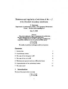
Security Constrained Unit Commitment With Dynamic Thermal Line Rating Mostafa Nick, Student Member, IEEE, Omid Alizadeh-Mousavi, Rachid Cherkaoui, Senior Member, IEEE, and Mario Paolone, Senior Member, IEEE

Abstract—The integration of the dynamic line rating (DLR) of overhead transmission lines (OTLs) in power systems security constrained unit commitment (SCUC) potentially enhances the overall system security as well as its technical/economic performances. This paper proposes a scalable and computationally efficient approach aimed at integrating the DLR in SCUC problem. The paper analyzes the case of the SCUC with AC load flow constraints. The AC-optimal power flow (AC-OPF) is linearized and incorporated into the problem. The proposed multi-period formulation takes into account a realistic model to represent the different terms appearing in the Heat-Balance Equation (HBE) of the OTL conductors. In order to include the HBE in the OPF, a relaxation is proposed for the heat gain associated to resistive losses while the inclusion of linear approximations are investigated for both convection and radiation heat losses. A decomposition process relying on the Benders decomposition is used in order to breakdown the problem and incorporate a set of contingencies representing both generators and line outages. The effects of different linearization, as well as time step discretization of HBE, are investigated. The scalability of the proposed method is verified using IEEE 118-bus test system.

Fitted line for

Fitted line for radiation heat loss

.

Conductor resistive heat gain [MW/m]. Conductor convection heat loss [MW/m]. Conductor radiation heat loss [MW/m]. Conductor resistance

.

B. Indices and sets Index of normal/contingency operation conditions ( normal operation). Generating units. Transmission lines between buses and . Network buses. Elements of piecewise linearized model of radiation heat loss. Elements of piecewise linearized model of . Benders decomposition iteration.

Index Terms—AC optimal power flow, Benders decomposition, convex formulation, Heat Balance Equation (HBE).

Time.

NOMENCLATURE

Set of generation units connected to bus .

A. Functions Active and reactive power generation cost [$/h]. Generating unit start-up cost [$].

C. Parameters Line shunt susceptance [p.u.]. Conductor diameters [mm]. Line longitudinal conductance and susceptance [p.u.]. Conductor altitude above sea level [m].

Generating unit shut down cost [$]. , ,

linearization.

Reserve procurement cost [$/h]. Convection heat loss coefficient for high/low/zero wind speed [MW/mK].

Base value of current. Line radiation heat loss coefficients MW/mK . Solar radiation heat gain coefficients [m].

Manuscript received October 20, 2014; revised February 05, 2015, April 05, 2015, and May 01, 2015; accepted June 09, 2015. The research illustrated in this manuscript has been carried out within the context of the project “Temperaturabhãngige Kapazitãtsausnutzung fũr Freileitungsnetze (TeKaF)” financed by the Swiss Competence Center Energy and Mobility (CCEM). Additionally, this research is framed within the activities of the Swiss Competence Center for Energy Research - Future Swiss Electrical Infrastructure (SCCER-FURIES). Paper no. TPWRS-01449-2014. The authors are with École Polytechnique Fédérale de Lausanne (EPFL), Lausanne, Switzerland. Color versions of one or more of the figures in this paper are available online at http://ieeexplore.ieee.org. Digital Object Identifier 10.1109/TPWRS.2015.2445826

,

Generating unit maximum/minimum power output [p.u.]. Bus demands [p.u.]. Line solar heat gain [MW/m]. Solar radiation MW . Conductor resistance at temperature . Ambient temperature [K]. Line reference temperature [K].

0885-8950 © 2015 IEEE. Personal use is permitted, but republication/redistribution requires IEEE permission. See http://www.ieee.org/publications_standards/publications/rights/index.html for more information.

This article has been accepted for inclusion in a future issue of this journal. Content is final as presented, with the exception of pagination. 2

IEEE TRANSACTIONS ON POWER SYSTEMS

Line maximum temperature [K]. , ,

Lower/upper bounds of conductor temperature for piecewise linearization of radiation heat loss [K]. Nodal voltage maximum/minimum amplitude [p.u.]. Conductor thermal resistivity coefficient . Weather emissivity. Wind speed [m/s]. Line heat capacity [MJ/mK]. HBE time step discretization [s].

D. Variables Line current flow amplitude [p.u.]. , ,

Generating unit active/reactive output [p.u.]. Line active/reactive power flows [p.u.]. Generating unit maximum reactive power available in case of contingency [p.u.]. Generating unit up/down regulation reserve [p.u.]. Up/down regulation reserve used in contingency [p.u.]. Transmission line temperature [K].

,

Conductor temperature for each segment of radiation heat loss linearization [K]. Generating unit on/off binary variables. Binary variable for radiation heat loss. ,

Bus voltage amplitude/angle. Auxiliary variables to model sub-problem cuts in master problem ( normal operation). I. INTRODUCTION

T

HE power transfer limit of overhead transmission lines (OTLs) is an important constraint for power systems planning and operation. This constraint plays an essential role in the secure and economic management of power systems. Even if this limit should be expressed in terms of the temperature of the line conductors, in practice the thermal limits are transformed in current constraints (i.e., the ampacities) via the Heat Balance Equation (HBE) or, also, in terms of maximum transmitted apparent power. Traditionally, thermal ratings are calculated seasonally assuming given conservative weather conditions [1]. These ratings mostly lead to conservative operational limits. However, there might be cases in which the static line rating (SLR) overestimates the real ones due to extreme weather conditions [1]. On the other hand there are methods to assess the so-called dynamic line rating (DLR). They can be briefly classified in 1) DLR forecast from power systems load and weather prediction [2], [3], 2) DLR estimation from indirect measurements [4], and 3) real-time DLR evaluation using integrated meteorological data [5].

The DLR can be incorporated in optimal power flow (OPF) problems in different time scales ranging from planning to realtime operation of power systems. Recent papers have investigated the effect of the DLR on wind power generation integration into power systems [6]. The general idea is to profit from the potential correlation between increased wind farm power output and increase of line rating of nearby overhead lines. Concerning this specific subject, in [7] the incorporation of the DLR has been considered in the planning stage to evaluate the increase of the potential level of wind power integration. In the system operation, the utilization of the DLR has studied in order to allow a reduction in the required spinning reserve [8], reducing wind power spillage [8], [9], and avoiding the re-dispatch of generating units and load shedding [7]. The improvement provided by the available transfer capacity (ATC) considering DLR instead of SLR is discussed in [10]. In spite of several advantages, the main obstacle to the widespread utilization of DLR is that HBE adds a set of time-coupled nonlinear equality constraints to OPF problems. Consequently, it increases the complexity of problems limiting the scalability of the solution methods. This issue has been addressed in some research papers using a simplified model of the electro-thermal coordination (ETC) [11], and an iterative linearized ETC [12], [13]. In order to reduce the complexity of the problem, in [11] the terms in HBE that are unrelated to power flow losses (i.e., the HBE solar, convection and radiation terms) are supposed constant with respect to the temperature. In view of this approximated assumption, the first order nonlinear differential HBE is replaced with a set of nonlinear inequalities. The iterative linearized ETC is proposed in [12] and [13]. The studied OPF problem is broken down in several linearized sub-problems whose solutions are iteratively linked. The line flows and the heat terms of HBE are linearized as function of the generating unit output power and the conductor temperature. In this approach the linearized HBE is only considered for a set of the lines that are operated near bounding constraints. Despite some efforts in the above-listed literature for the integration of DLR into OPF problems, the methods are usually over-simplified, non-convex or the solutions are obtained iteratively with associated non-negligible computational aspects that limit their applicability. Another drawback of the available literature is related to the security of the system. The DLR is more beneficial in case where contingencies are accounted. Thus, a security constrained unit commitment (SCUC) including DLR should be used [14]. Moreover, the effects of reactive power flow and voltage limitations must be taken into account. These necessities require the use of the AC load flow (ACLF) equations that is not adopted in the current literature dealing with this problem. The main contributions of this paper are: 1) formulation of a SCUC with linearized AC constraints and DLR, 2) investigation of different terms of HBE and their incorporation with a realistic model of HBE into SCUC, 3) investigation of scalability of the proposed method, and 4) discussion of the robustness of the proposed methodology performing various sensitivity analyzes (e.g. piecewise-linear approximation versus linear approximation, time step discretization of HBE).

This article has been accepted for inclusion in a future issue of this journal. Content is final as presented, with the exception of pagination. NICK et al.: SECURITY CONSTRAINED UNIT COMMITMENT WITH DYNAMIC THERMAL LINE RATING

The structure of the paper is the following: Section II presents the basic aspects of DLR of OTLs with reference to HBE. With reference to the day-ahead scheduling problem, Section III illustrates the developed formulations and solution approaches capable to include the HBE into the AC-SCUC problem. The case studies and discussions on practical implementation of the proposed approaches are provided in Section IV. Finally, Section V concludes the paper with the final remarks summarizing the main findings. II. BASIC ASPECTS OF DYNAMIC RATING OF TRANSMISSION LINES: HEAT BALANCE EQUATION Before summarizing the basic aspects of the DLR of OLTs, it is worth mentioning that the current-temperature relationship of OTL conductors is discussed by the IEEE Std. 738 [15] and the CIGRE SC.B2 WG 22.12 [16]. These two standards are compared in [9] with the purpose of demonstrating that they provide essentially the same results. It is assumed that the conductor cross sections are circular. According to IEEE Std. 738, the overhead line temperature depends on 1) current flowing through the conductor, 2) conductor size and resistance, and 3) ambient weather conditions (e.g., temperature, wind speed and direction, solar radiation) [1]. The HBE relates the rates at which thermal energy enters, leaves and gets stored in the conductor. The heating terms are the resistive losses and the solar heat gain, while the cooling ones are the convection and the radiation terms. The relationship between the conductor temperature changes with respect to the received net thermal energy can be formulated using the HBE (1) which is a first-order nonlinear differential equation [15]:

(1) The ohmic losses that produce the heat in the conductor link the electrical and thermal variables. This term, shown in (2), alongside with solar heat gain, (3), are the heating sources that cause the temperature rise of the conductor [15]: (2) (3)

3

The remaining two terms, convection and radiation heat losses, are the ones that cool down the conductor. These two terms can be represented as a function of the conductor temperature for each generic weather condition (i.e., wind speed, altitude and ambient temperature) as they are shown in (4) and (5) [15] at the bottom of the page. Equations (2), (4), and (5) make the SCUC problem highly non-linear, non-convex and, consequently, hard to solve. In the following section we first formulate the targeted SCUC problem and, afterwards, we propose a methodology to effectively solve the AC-SCUC problem including HBE. III. PROBLEM DEFINITION In what follows we discuss the incorporation of the HBE in the multi-period day-ahead scheduling problem. The day-ahead scheduling problem can be solved with different objective functions like, for instance, the minimization of total generation cost or the maximization of the social welfare. We have focused on the former case. The generation scheduling problem for the day-ahead is accomplished performing a SCUC. In the proposed formulation the power balance equations are modeled with linearized AC load flow equations (ACLF). A. Day-Ahead Scheduling We assumed the perfect knowledge of the cost coefficients of the generating units. In addition to the total production cost of the active and reactive powers of the generation units and their respective reserve provision costs, their start-up and shut-down costs are also included in the objective function (6a). The ramp up/down constraints, minimum up/down time constraints and start-up/shut-down constraints are taken into consideration according to [17]. The other constraints represent the normal operating conditions and the contingency states of the system. Note that active/reactive power load balances at each node for the normal operating point and the contingencies are given with (6c)/(6e) and (6d)/(6f), respectively. The active and reactive power flows over each line are shown with equations (6g) and (6h),1 respectively. The maximum and minimum active power production limits of each generating unit are represented by constraints (6i) and (6j). The upper limits of upward and downward 1Note that in (6h), the correct line representation (using ered since the transverse parameters are included.

model) is consid-

zero wind

(4a)

non-zero wind

(4b)

(5)

This article has been accepted for inclusion in a future issue of this journal. Content is final as presented, with the exception of pagination. 4

IEEE TRANSACTIONS ON POWER SYSTEMS

reserves are given by (6k) and (6l). The reactive power production limits of every generating units is given by (6m). The constraint (6n) models the current flow over transmission lines (it is assumed that the voltage is 1 p.u.). The equation (6o) represents the nodal voltage upper and lower limits. The HBE is shown with equation (6p) and the maximum temperature limit of thelines is represented by (6q). The units on/off state is represented by equation (6r).2

(6a)

(6b) (6c)

(6d) (6e)

(6f)

(6g)

(6h) (6i) (6j) (6k) (6l) (6m) (6n) (6o)

(6p) (6q)

(6r) 2In the formulation of the problem, we have neglected the possibility to temporarily overload the lines following a given contingency.

(6s) (6t) This problem is a large-scale mixed integer nonlinear, and non-convex one and is hard to solve. In the next sub-sections we propose a procedure to deal with these difficulties. B. Investigation of HBE Convexification The solar heat gain term in HBE is given for each generic weather condition but the other three terms are non-convex and are required to be convexified. The heat gain related to the ohmic losses is proportional to the square of the current flow in the conductor and its resistance. The latter is a function of the conductor temperature (for an ohmic conductor) as it is shown in (7). In order to convexify the ohmic losses heat gain, given in (2), we have: 1) considered that the resistance of the conductor is constant at its value at the maximum temperature3 (conservative hypothesis), 2) considered the voltage is close to 1 p.u. therefore the current flow is equal to the apparent power flow [equation (6n)], 3) and finally we relaxed the equality constraint (2) to an inequality one given in (8): (7) (8) This relaxation is exact with respect to the considered approximations since this inequality constraint will be identical to the equality one when the conductor temperature constraint (6q) is binding. The convection heat loss is a function of wind speed, ambient temperature, altitude and internal conductor temperature. As shown in Fig. 1, in the case of non-zero wind speed the relations between this heat loss and the conductor temperature at each generic wind speed and the ambient temperate is linear. However, the convection heat loss function is different for high and low wind speeds and the one producing the largest heat losses should be used [15]. If it is written as a function of the difference between the internal conductor temperature and the ambient temperature, in equation (4b) we can use the maximum of the slope calculated for high and low wind speeds. In this study we did not model the case of non-zero wind speed because: 1) the non-zero wind speed occurs rarely and 2) a very small wind speed always can be used instead of zero wind. In addition, the zero wind speed equation can be easily linearized or piecewise-linearized. The radiation heat loss can be piecewise linearized. This approximation is shown in Fig. 2 with three lines.4 The equation 3Since, in general, the network operator is interested to better exploit the lines when they reach their maximum operating temperatures, we decided to make this conservative assumption. Its indirect effect is that the error introduced by such an approximation is progressively reduced when the conductor temperature comes closer to its maximum limit. 4The radiation heat loss depends on the power four of the conductor temperature as shown in equation (5). In order to piecewise linearize this cooling term, it is written as a function of the conductor temperature with a domain between the maximum conductor temperature and the ambient temperature. The piecewise linearization is done with evenly dividing the domain into the total number of desired pieces.

This article has been accepted for inclusion in a future issue of this journal. Content is final as presented, with the exception of pagination. NICK et al.: SECURITY CONSTRAINED UNIT COMMITMENT WITH DYNAMIC THERMAL LINE RATING

5

Fig. 3. Flowchart of the proposed method. Fig. 1. Linear relationship for convection heat loss in case of non-zero wind . speed

Fig. 2. Piecewise-linearization of radiation heat loss

.

(9) is added to the problem instead of (5) in order to piecewise-linearize the radiation heat loss term in HBE: (9a) (9b) (9c) (9d)

required to breakdown the problem into smaller ones. The benders decomposition methodology is used here to decompose the original problem. This approach is widely used to solve power system problems (e.g., [14]). The process of the benders decomposition applied to our problem is as depicted in Fig. 3. The first stage (master problem) commits the generation units (UC) and provides economic dispatch (ED) to minimize the operation cost including the active and reactive power generation cost in addition to up-regulation and down-regulation reserve procurement. The network security check for the normal case and the contingency scenarios are verified in the second stage (subproblems). Since the subproblems are independent from each other, they can be processed simultaneously in parallel. In each iteration if the security constraints are violated, an appropriate cut will be generated and added to the master problem. 1) Unit Commitment (Master Problem): The initial master problem disregards the security constraints and provides an initial schedule for the generation units. Its objective function is shown in (10a) and its constraints are active and reactive load balances, ramp up/down constraints, minimum up/down time constraints and start-up/shut-down constraints. A set of appropriate cuts representing the security costs is added to it at each iteration:

(9e) The proposed piecewise-linearization approximations for the radiation can be replaced with a linear approximation. We have used the linearized model (one line instead of several lines) to avoid binary variables. In Section IV, we will show that this approximation brings a very small error and effectively decreases the computational time.

(10a)

C. Security Constrained Unit Commitment With AC Load Flow and HBE The OPF is a known but challenging problem since it is, in general, non-convex and hard to solve. In this respect several approaches, like Semi definite programming (SDP), second order cone programming (SOCP) relaxations [18], and linearization methods using the Newton-Raphson method [14], have been proposed. Recently, a linearized AC load flow was proposed in [19] which is an extension of DC load flow. In this paper we adapt its methodology to formulate the AC-SCUC with HBE. Even with the linearized model, the SCUC is still a very large-scale problem with binary variables and very hard and time consuming to be solved. The inclusion of contingencies will even make it harder. Therefore, decomposition methods are

(10b) (10c) (10d) (10e) (10f) (10g) (10h)

This article has been accepted for inclusion in a future issue of this journal. Content is final as presented, with the exception of pagination. 6

IEEE TRANSACTIONS ON POWER SYSTEMS

The are the slack variables for active and reactive power balances at each node. The and are large numbers. The constraints of the normal operating condition and contingencies set are (15b)–(15h) and (15i)–(15q), respectively. The parameters indicated with are obtained from the solution of the previous master problem. Constraints corresponding to the normal operating conditions : Fig. 4. Linearization of

.

The solution of this optimization problem will be fixed and used in the subproblems. 2) Network Security Check (Subproblems): The network security must be checked for the obtained dispatch in the master problem. This security check is done for the normal operating condition as well as the set of contingencies. The AC load flow problem is used here. However, in order to formulate a convex sub-problem, we have linearized it. The linearized AC load flow is described below [19]. The main ideas of the linearized AC load flow are 1) approximate by , 2) by a set of linear constraints, and 3) decompose the nodal voltages into a fixed value (normally 1 p.u.) and a small variation. The is piecewise linearized. Then to avoid binary variables, these set of piecewise linearized constraints are relaxed from equality constraints to inequality ones as shown in Fig. 4 and also in equation (11). This relaxation is most of the time exact otherwise the reactive and active power losses over the lines will increase:

(15b)

(15c) (15d) (15e) (15f) (15g) (15h) Constraints expressed for any possible considered contingency (i.e., lines and/or generators outages) :

(15i)

(11) The voltage of the nodes can be written as (12) in two parts, one fixed and one variable: (12)

(15j)

Substituting the nodal voltages and relaxed-linearized model of according to (11) and (12) in (6h) and using the Taylor expansion, the reactive flow can be approximated as (13):

(15k) (15l) (15m) (15n) (15o)

(13)

(15p)

Similarly, the active power flow can be approximated as (14):

(15q)

(14)

are the dual of the conThe straints (15e), (15n), (15o), (15f), and (15l), respectively. After solving the subproblems, the following cuts are generated and added to the next iteration of the master problem:

Once the schedule is done in the master problem, the obtained solution (active and reactive productions and reserve capacities) will be fixed and used in the subproblems. The dual of these constraints will be used to generate appropriate cuts for the master problem. The objective function of the subproblems for both normal and contingency conditions is as in (15a):

(15a)

(16a)

This article has been accepted for inclusion in a future issue of this journal. Content is final as presented, with the exception of pagination. NICK et al.: SECURITY CONSTRAINED UNIT COMMITMENT WITH DYNAMIC THERMAL LINE RATING

7

TABLE I DATA OF GENERATING UNITS FOR 5-BUS SYSTEM [13]

The described procedure iterates until it converges to the optimal solution and all the slack variables have zero values. The master problem is mixed-integer quadratic programming (MIQP) whereas the subproblems are quadratically constrained optimization ones (QCP). These types of optimization problems can be easily solved using conventional optimization software. Here, these problems are solved using the solver Gurobi [21] via the MATLAB interface YALMIP [22].5 IV. CASE STUDIES AND PRACTICAL IMPLEMENTATION OF PROPOSED MODELS

Fig. 5. Single line diagram of 5-bus system. TABLE II SIMULATION PARAMETERS FOR 5-BUS SYSTEM

(16b)

This section shows the effectiveness of the proposed HBE inclusion into AC-SCUC by making reference to different case studies. For the sake of clarity, the first one is a “toy example” composed of 5 buses and 6 lines [13]. The IEEE 118-bus test case is then used to show the scalability of the proposed method. The HBE based DLR (HBE-DLR) is compared with MVA 6 ampacity based DLR (MVA-DLR) and SLR. In the MVA-DLR, an independent and fixed ampacity is calculated for every conductor at each time step based on forecasted weather parameters. It should be noted that there are two time steps. One is for the 24-h unit commitment (so, based on the hourly dispatch) while the second one is for HBE discretization which can be 1, 5, 10, 12, 15, 20, and 30 min. A. Description of the Test System and Weather Parameters

(16c) The indicates the values obtained from the solution of the sub-problems. It should be noted that in case of normal operating conditions, one cut is created per time period. Therefore, in each iteration of Benders decomposition 24 constraints (total number of time periods) are added to the master problem. For the contingency scenarios, two cuts are produced for each time period. The cuts for the contingency cases are separated with respect to the up and down regulation reserves in order to produce more appropriate cuts for the master problem. The [the positive slack variable of the active power in the load balance equation (15i)] will not get a non-zero value due to the down regulation constraint (15o). Similarly will not get a positive value due to the up regulation constraint (15n). Therefore, the cuts can be separated with respect to the dual of these two constraints and the part of the objective function (15a) that includes , and . This decreases the required number of iterations for the convergence of the Benders decomposition algorithm [20].

The single line diagram of the 5-bus system is shown in Fig. 5. This network includes three loads and four generating units. The data of generating units is given in Table I. The maximum amount of loads are equal to 280 MW, 300 MW, and 290 MW with a power factor of 0.95. The reactance of the transmission lines is equal to . The conductor diameters are assumed equal to 26.1 mm. The base values for apparent power and voltage are 100 MVA and 230 kV, respectively. The hourly profiles of ambient temperature, wind speed, load and solar irradiation used for this case study are shown in Figs. 6 and 7.7 It should be noted that these temperature profiles are for the lines 1 and 2. With respect to these profiles, the temperature profiles of the lines 3 and 5 are in average 3 warmer and the temperature profile for lines 4 and 6 are in 5It should be noted that the subproblems are QCPs. The resistive heat losses are the quadratic constraints [8]. In some cases, optimization solvers may fail to compute the duals of the QCP problem. To prevent this problem, these quadratic . In this way the subproblems constraints can be piecewise linearized like will become linear. 6The lines transfer capacity are expressed in terms of maximum transmitted apparent power. 7These weather conditions makes reference to a potential summer scenario with a clear sky of a line placed in a central region of Europe.

This article has been accepted for inclusion in a future issue of this journal. Content is final as presented, with the exception of pagination. 8

IEEE TRANSACTIONS ON POWER SYSTEMS

TABLE III SIMULATION RESULTS FOR 5-BUS SYSTEM USING PIECEWISE LINEAR AND LINEAR APPROXIMATIONS

Fig. 6. Daily active load in per unit (Base value perature profiles.

100 MW) and ambient tem-

Fig. 8. Conductor temperatures evolution for 5-bus system using linear approximation. Fig. 7. Daily wind speed and solar radiation profiles.

average 5 colder. Other simulation parameters are shown in Table II. They are assumed to be the same for all the lines. In Sections IV-B and IV-C the maximum conductor temperature is considered to be 100 while in Sections IV-D and IV-E, it is considered to be 80 . The quadratic term of the generation cost function is neglected in these two former sub-sections. B. Influences of the HBE Modeling This sub-section discusses the impacts of linearization approximations and time step discretization of the HBE model. For this purpose, these two aspects are studied with 5-bus system and using a DC Load Flow (DCLF) assumption regardless of the N-1 security criterion. 1) Comparison of Piecewise Linearization versus Linearization Model of Radiation Heat Loss: In Section III-B it is shown that the radiation and convection (in case of zero wind speed) heat losses can be accurately modeled with piecewise-linearized models. These models introduce additional binary variables to the problem. Here, it is shown that the use of the linearized models, instead of piecewise-linearized ones, significantly decreases the computation time keeping the errors relatively small (In order to have zero wind speeds, the wind speeds at hours 4 and 14 are assumed to be zero in the profile shown in Fig. 7.). The simulation results in Table III show that the error of the identified minimum of the objective function for the case of linear HBE approximation is less than 0.2% with an associated computation time that is significantly reduced. It should be noted that the time step discretization of HBE is chosen to be 30 min. The temperature evolutions of the lines are shown in Fig. 8 for the linearized models. It should be noted that these temperature profiles are a-posteriori calculated and based on the HBE formulation given by the IEEE Std. [15]. Fig. 8 shows that the maximum temperature reached for the case of the linear HBE approximation is 97.41 (since a conservative linearization

Fig. 9. Evolution of conductor temperatures error for 5-bus system using linear approximation for L2 and L3.

was selected). It can be observed that the linear approximation is conservative for temperatures below the maximum and tends to guarantee a better security of the system. Fig. 9 shows the conductor temperatures for lines L2 and L3 concerning two cases: 1) those calculated a-posteriori with original IEEE std. model [15] and 2) those obtained from the optimization problem with linearized approaches. It can be observed that the temperature errors are negligible and they are in the conservative region8 (the conductor temperatures calculated with the realistic model are lower than the approximated ones). The above results show that the use of linearized models will decrease the computation time significantly while introducing a negligible error. This improvement in the computation time is highly important for the case of large-scale networks. 2) Influence of HBE Time-Step Discretization: In IEEE standard [15], it is recommended that “for accurate dynamic calculation the time step chosen should be sufficiently small with respect to the thermal time constant of the conductors. It is always prudent to rerun the calculation with a smaller time step to check whether the calculated values change.” 8These errors are due to two main reasons: 1) linearization of radiation heat loss and 2) approximation of resistance of the conductors being at their maximum value.

This article has been accepted for inclusion in a future issue of this journal. Content is final as presented, with the exception of pagination. NICK et al.: SECURITY CONSTRAINED UNIT COMMITMENT WITH DYNAMIC THERMAL LINE RATING

9

TABLE IV SIMULATION RESULTS FOR THE 5-BUS SYSTEM CONCERNING DIFFERENT TIME STEPS SELECTED TO DISCRETIZE THE HBE

TABLE V AMBIENT PARAMETERS FOR THE SLR

In this respect, this sub-section illustrates the effects of the HBE time step discretization on the obtained results. Table IV provides, for different time steps, the value of identified minimum objective function, the maximum conductor temperature and the computation time. It is observed that for smaller time steps the value of the objective function decreases. It is due to the fact that smaller time steps allow for a more accurate modeling of conductor temperature evolution. However, for smaller time steps the computation time increases significantly because the number of HBE constraints increases. It should be noted that the selection of the HBE time step discretization depends on the thermal inertia of the conductors that is the dominant dynamic. This parameter does not change with the power system size (i.e., number of nodes). Therefore, they can be chosen a-priori. As it can be seen from the results shown in Table IV, the value of the objective function for the time step equal to 30 minutes is 0.1% higher than the one obtained for the time step equal to 1 min, whereas its computation time is 18.3 times lower. C. Comparison of HBE-DLR with MVA-DLR and SLR Using DCLF The 5-bus system has been used to compare the results of HBE-DLR with SLR and MVA-DLR. For the case of SLR, the maximum ampacity of conductors are calculated according to IEEE Std. [15] and using the given ambient parameters of Table V. The optimal identified value of the objective function and maximum conductor temperatures for SLR, HBE-DLR and MVA-DLR are shown in Table VI. For these three cases, the generating units' commitment and their output power, line temperature profiles and heat balance terms profile are shown in Fig. 10. Table VI shows that SLR has the highest value of the objective function since the transmission capacities are obtained for the conservative weather parameters. On the other hand, MVA-DLR has the lowest value of the objective function. However, a-posteriori calculated conductor temperatures shown in Fig. 10.b.2 demonstrates that this scheduling does not respect the maximum allowed conductors' temperature. It is due to the fact that the MVA-DLR ignores the dynamics of conductors' temperature as well as their initial temperature (from the previous time step). In other terms, the dynamic term in the equation (1) is neglected and the temperature can overpass the dedicated limit. The obtained results using the proposed HBE-DLR has the lowest secure objective function value. As it can be seen

TABLE VI OBJECTIVE FUNCTION VALUE AND MAXIMUM CONDUCTOR TEMPERATURES FOR 5-BUS SYSTEM AND FOR SLR, MVA-DLR, AND HBE-DLR

from Fig. 10.b.3, the maximum conductors' temperature limits has been effectively respected over all time periods. The heat loss/gain terms of HBE for the three cases are shown in Fig. 10.c and 10.d. The heat gain/loss terms of HBE for the HBE-DLR, shown in Fig. 10.c.3 and 10.d.3, demonstrates that the management of the power flows between high loaded line (like L1) and low loaded line (like L3) decreases the value of objective function while the maximum allowed conductor temperatures is respected. The similar trends can be observed for the MVA-DLR in heat balance terms, as shown in Fig. 10.c.2 and 10.d.2. However, since the dynamics of the HBE equation is not considered, the conductor temperature exceeds the allowed level. For the case of SLR, as shown in Fig. 10.c.1 and 10.d.1, such behaviors have not been observed in the heat balance terms. D. Comparison of HBE-DLR versus MVA-DLR in AC-SCUC The 5-bus system has been used to compare the results of HBE-DLR with MVA-DLR. The maximum allowed temperature of the conductors is chosen to be 80 . As it was shown in previous sub-section, MVA based DLR could result in insecure operation condition. In order to prevent the overloading of the conductors, the maximum MVA rating of the conductors is calculated with 75 as the maximum conductor temperatures. In order to prevent load shedding the load and the solar irradiation profiles used in the previous sub-section are decreased by 10% and 40% respectively. The N-1 criteria is used to evaluate the security of the system for the set of generation units and transmission lines outages (in total 10 contingencies for each hour (4 generation units and 6 transmission lines). The master problem is the same for both MVA-DLR and HBE-DLR while the differences are in the subproblems. They depend on whether we are using HBE-DLR or MVA-DLR. The value of the objective function and the computation time using MVA-DLR and HBE-DLR cases are given in Table VII. It shows that the use of the HBE-DLR in conjunction with the proposed AC-SCUC approach decreases the value of the identified minimum objective function as well as the number of iteration between the master and subproblems. The generation units power output, upward reserve, and downward reserve for both cases are shown in Fig. 11. It shows how the units are scheduled to maintain the conductors' security while their maximum capacity is exploited.

This article has been accepted for inclusion in a future issue of this journal. Content is final as presented, with the exception of pagination. 10

IEEE TRANSACTIONS ON POWER SYSTEMS

Fig. 10. Generating units’ output power, line temperature profiles, and heat balance terms profile for 5-bus system for SLR, MVA-DLR, and HBE-DLR ( min). TABLE VII COMPARISON OF HBE-DLR WITH MVA-DLR IN AC-SCUC

TABLE VIII COMPARISON OF HBE-DLR WITH SLR AND MVA-DLR IN AC-SCUC USING 118-BUS NETWORK

E. Investigation of the Scalability of the Proposed Method In this sub-section, the proposed AC-SCUC model with HBE inclusion is analyzed with IEEE 118-bus test system in order to investigate the scalability of the proposed approach. In order to prevent load shedding the ambient temperature and the solar irradiation profiles used in the previous sub-section are decreased by 20% and 40% respectively. The set of contingencies includes all the generation units (54 units) and all the transmission lines (179 lines) which results in total 233 contingencies for each hour. The results of the simulation for the cases using HBE-

DLR, MVA-DLR, and SLR are shown in Table VIII. This table shows that the identified minimum of the objective function decreases with HBE-DLR and its overall computation time decreases as well (the computation time for both master and subproblems shown in this table are the average of the all iteration.). It is worth mentioning that although the computation time for HBE-DLR is the highest one, its number of Benders decomposition is reduced. This behavior is driven by the fact that the HBE-DLR makes the subproblem feasible solution space larger

This article has been accepted for inclusion in a future issue of this journal. Content is final as presented, with the exception of pagination. NICK et al.: SECURITY CONSTRAINED UNIT COMMITMENT WITH DYNAMIC THERMAL LINE RATING

11

Fig. 11. Generation units scheduling for HBE-DLR (a) and MVA-DLR (b) (a1 and b1 the active power output, a2 and b2 the upward reserve, a3 and b3 the downward reserve).

and,sincetheBendersiterationsarecontinueduntilallthesecurity violations are removed, this allows to reach the feasibility faster. V. CONCLUSIONS The incorporation of HBE in optimal scheduling of power systems is a challenging task since the HBE brings a set of nonlinear and time-coupled equality constraints to the AC-SCUC. This paper proposes an efficient and appropriate way to integrate the HBE in AC-SCUC problems. In this respect the radiation and convection heat losses equations are linearized and a quadratic relaxation is proposed for resistive heat gains of the conductors. On other hand, linearized AC-OPF equations are used to take into account the non-negligible impacts of reactive power flow and voltage constraints. A decomposition process relying on the Benders decomposition has been presented in order to enable the possibility to breakdown the problem and incorporate a set of contingencies representing both generators and line outages. Various sensitivity analysis have been performed to show the effectiveness of the proposed model and the impact of different modeling approach (i.e., HBE discretization time step, linear versus piecewise linear HBE approximations). The advantages of the proposed model for optimality, computation time, and system security are demonstrated. Finally, the scalability of the proposed approach is illustrated using as benchmark network the IEEE 118-bus test system. REFERENCES [1] T. Goodwin and C. Smith, “Smart Grid Demonstration Project—Dynamic Line Rating (DLR)—Oncor Electric Delivery,” in ERCOT Region Operations Training Seminar, 2011. [2] D. Kim, J. Cho, H. Lee, H. Jung, and J. Kim, “Prediction of dynamic line rating based on assessment risk by time series weather model,” in Proc. PMAPS, Stockholm, Sweden, 2006. [3] E. Siwy, “Risk analysis in dynamic thermal overhead line rating,” in Proc. PMAPS, Stockholm, Sweden, 2006. [4] M. RuiKun, F. Ling, and X. HaiBo, “Dynamic line rating estimator with synchronized phasor measurement,” in Proc. Int. Conf. Advanced Power Syst. Automation and Protection, Beijing, China, 2011. [5] S. Foss, S. Lin, and R. Fernandes, “Dynamic thermal line ratings Part I: Dynamic ampacity rating algorithm,” IEEE Trans. Power App. Syst., vol. PAS-102, no. 6, pp. 1858–1864, 1983. [6] S. Abdelkader, S. Abbott, J. Fu, B. Fox, D. Flynn, L. McClean, and L. Bryans, “Dynamic monitoring of overhead line ratings in wind intensive areas,” in Proc. Eur. Wind Energy Conf. Exhib., Marseille, France, 2009.

[7] T. Ringelband, M. Lange, M. Dietrich, and H. -J. Haubrich, “Potential of improved wind integration by dynamic thermal rating of overhead lines,” in Proc. IEEE PowerTech, Bucharest, Romania, 2009. [8] B. Banerjee, D. Jayaweera, and S. Islam, “Impact of wind forecasting and probabilistic line rating on reserve requirement,” in Proc. IEEE POWERCON, Auckland, New Zealand, 2012. [9] M. Simms and L. Meegahapola, “Comparative analysis of dynamic line rating models and feasibility to minimize energy losses in wind rich power networks,” Energy Convers. Manage., vol. 77, pp. 11–20, 2013. [10] M. Miura, T. Satoh, S. Iwamoto, and I. Kurihara, “Application of dynamic rating to evaluation of ATC with thermal constraints considering weather conditions,” in Proc. IEEE Power Eng. Soc. General Meeting, Montreal, QC, Canada, 2006. [11] M. Wang and X. Han, “Study on electro-thermal coupling optimal power flow model and its simplification,” in Proc. IEEE Power & Energy Soc. General Meeting, Minneapolis, MN, USA, 2010. [12] H. Banakar, N. Alguacil, and F. Galiana, “Electrothermal coordination Part I: Theory and implementation schemes,” IEEE Trans. Power Syst., vol. 20, no. 2, pp. 798–805, May 2005. [13] N. Alguacil, M. Banakar, and F. Galiana, “Electrothermal coordination Part II: Case studies,” IEEE Trans. Power Syst., vol. 20, no. 4, pp. 1738–1745, Nov. 2005. [14] F. Yong, M. Shahidehpour, and L. Zuyi, “AC contingency dispatch based on security-constrained unit commitment,” IEEE Transc. Power Syst., vol. 21, no. 2, pp. 897–908, May 2006. [15] IEEE Std. 738-2006—IEEE Standard for Calculating the Current-Temperature of Bare Overhead Conductors, 2007. [16] “The thermal behavior of overhead line conductors,” Cigre Working Group 22. 12, 1992. [17] M. Carrión and J. Arroyo, “A computationally efficient mixed-integer linear formulation for the thermal unit commitment problem,” IEEE Trans. Power Syst., vol. 21, no. 3, pp. 1371–1378, Aug. 2006. [18] S. Low, “Convex relaxation of optimal power flow—Part I: Formulations and equivalence,” IEEE Trans. Control Netw. Syst., vol. 1, pp. 15–27, 2014. [19] C. Coffrin and P. Van Hentenryck, A linear-programming approximation of AC power flows. CoRR, abs/1206. 3614, 2012. [20] F. You and I. E. Grossmann, “Multicut Benders decomposition algorithm for process supply chain planning under uncertainty,” Ann. Oper. Res., vol. 210, pp. 191–211, 2013. [21] Gurobi Optimization, 2013 [Online]. Available: http://www. gurobi. com/ [22] J. Lofberg, “YALMIP: A toolbox for modeling and optimization in MATLAB,” in Proc. IEEE Int. Symp. Comput. Aided Control Syst. Design, Taipei, Taiwan, 2004.

Mostafa Nick (S’12) was born in Iran in 1986. He received the Master’s degree in electrical engineering from Amirkabir University of Technology (Tehran Polytechnic), Iran, in 2011. Currently, he is pursuing the Ph.D. degree in the Distributed Electrical System Laboratory (DESL) of the École Polytechnique Fédérale de Lausanne (EPFL), Lausanne, Switzerland. His research interests are power systems operation and planning, and distributed energy storage modeling and relevant applications.

This article has been accepted for inclusion in a future issue of this journal. Content is final as presented, with the exception of pagination. 12

Omid Alizadeh-Mousavi received the Ph.D. degree in electrical engineering from École Polytechnique Fédérale de Lausanne (EPFL), Lausanne, Switzerland, in 2014. His research interests are power systems operation and planning, and security and risk assessment.

Rachid Cherkaoui (SM’07) received the M.S. degree in electrical engineering and the Ph.D. degree from École Polytechnique Fédérale de Lausanne (EPFL), Lausanne, Switzerland, in 1983 and 1992, respectively. From 1992 to 2009, he was leading the research activities in the field of optimization and simulation techniques applied to electrical power and distribution systems. Since 2009, as senior scientist, he is the head of the power system group (PWRS) at EPFL. Presently, the main research topics of his group are concentrated on electricity market deregulation, distributed generation and storage with reference to distribution systems and smart grids, and power system vulnerability mitigation. He is the author or coauthor of more than 100 scientific publications.

IEEE TRANSACTIONS ON POWER SYSTEMS

Mario Paolone (M’07–SM’10) received the M.Sc. degree (with honors) and the Ph.D. degree in electrical engineering from the University of Bologna, Italy, in 1998 and 2002, respectively. In 2005, he was appointed assistant professor in power systems at the University of Bologna where he was with the Power Systems Laboratory until 2011. In 2010, he received the Associate Professor eligibility from the Politecnico di Milano, Italy. Currently, he is an Associate Professor at the Swiss Federal Institute of Technology, Lausanne, Switzerland, where he accepted the EOS Holding Chair of the Distributed Electrical Systems Laboratory. His research interests are in power systems with particular reference to real-time monitoring and operation, power system protections, power systems dynamics, and power system transients. He is author or coauthor of over 170 scientific papers published in reviewed journals and international conferences. Prof. Paolone is secretary and member of several IEEE and Cigré Working Groups. He was co-chairperson of the Technical Committee of the 9th edition of the International Conference of Power Systems Transients (IPST 2009). In 2013, he was the recipient of the IEEE EMC Society Technical Achievement Award. He is the Editor-in-Chief of the Elsevier journal Sustainable Energy, Grids and Networks.