From the viewpoint of machine learning, a time-series classification problem is basically a supervised ... and off-the-shelf time-series classification method. More precisely, the ..... In Advances in Neural Information Processing. Systems 14 ...
Segment and combine approach for non-parametric time-series classification Pierre Geurts† and Louis Wehenkel University of Li`ege, Department of Electrical Engineering and Computer Science, Sart-Tilman B28, B4000 Li`ege, Belgium, † Postdoctoral researcher, FNRS, Belgium {p.geurts,l.wehenkel}@ulg.ac.be
Abstract. This paper presents a novel, generic, scalable, autonomous, and flexible supervised learning algorithm for the classification of multivariate and variable length time series. The essential ingredients of the algorithm are randomization, segmentation of time-series, decision tree ensemble based learning of subseries classifiers, combination of subseries classification by voting, and cross-validation based temporal resolution adaptation. Experiments are carried out with this method on 10 synthetic and real-world datasets. They highlight the good behavior of the algorithm on a large diversity of problems. Our results are also highly competitive with existing approaches from the literature.
1
Learning to classify time-series
Time-series classification is an important problem from the viewpoint of its multitudinous applications. Specific applications concern the non intrusive monitoring and diagnosis of processes and biological systems, for example to decide whether the system is in a healthy operating condition on the basis of measurements of various signals. Other relevant applications concern speech recognition and behavior analysis, in particular biometrics and fraud detection. From the viewpoint of machine learning, a time-series classification problem is basically a supervised learning problem, with temporally structured input variables. Among the practical problems faced while trying to apply classical (propositional) learning algorithms to this class of problems, the main one is to transform the non-standard input representation into a fixed number of scalar attributes which can be managed by a propositional base learner and at the same time retain information about the temporal properties of the original data. One approach to solve this problem is to define a (possibly very large) collection of temporal predicates which can be applied to each time-series in order to compute (logical or numerical) features which can then be used as input representation for any base learner (e.g. [7, 8, 10, 11]). This feature extraction step can also be incorporated directly into the learning algorithm [1, 2, 14]. Another approach is to define a distance or similarity measure between time-series that takes into account temporal specific peculiarities (e.g. invariance with respect to Proceedings of the 9th European Conference on Principles and Practice of Knowledge Discovery in Databases (PKDD), Springer, 2005
time or amplitude rescaling) and then to use this distance measure in combination with nearest neighbors or other kernel-based methods [12, 13]. A potential advantage of these approaches is the possibility to bias the representation by exploiting prior problem specific knowledge. At the same time, this problem specific modeling step makes the application of machine learning non autonomous. The approach investigated in this paper aims at developing a fully generic and off-the-shelf time-series classification method. More precisely, the proposed algorithm relies on a generic pre-processing stage which extracts from the timeseries a number of randomly selected subseries, all of the same length, which are labeled with the class of the time-series from which they were taken. Then a generic supervised learning method is applied to the sample of subseries, so as to derive a subseries classifier. Finally, a new time-series is classified by aggregating the predictions of all its subseries of the said size. The method is combined with a ten-fold cross-validation wrapper in order to adjust automatically the size of the subseries to a given dataset. As base learners, we use tree-based methods because of their scalability and autonomy. Section 2 presents and motivates the proposed algorithmic framework of segmentation and combination of time-series data and Section 3 presents an empirical evaluation of the algorithm on a diverse set of time-series classification tasks. Further details about this study may be found in [4].
2
Segment and Combine
Notations A time-series is originally represented as a discrete time finite duration real-valued vector signal. The different components of the vector signal are called temporal attributes in what follows. The number of time-steps for a given temporal attribute is called its duration. We suppose that all temporal attributes of a given time-series have the same duration. On the other hand, the durations of different time-series of a given problem (or dataset) are not assumed to be identical. A given time series is related to a particular observation (or object). A learning sample (or dataset) is a set (ordering is considered irrelevant � � at this level) of N preclassified time-series denoted by LSN = a(td(o) , o), c(o) o = 1, . . . , N , where o denotes an observation, d(o) ∈ IN stands for the duration of the timeseries, c(o) refers to the class associated to the time-series, and a(td(o) , o) = (a1 (td(o) , o), . . . , an (td(o) , o))0 , ai (td(o) , o) = (ai (1, o), . . . , ai (d(o), o))0 , represents the vector of n real-valued temporal attributes of duration d(o). The objective of the time-series classification problem is to derive from LSN a classification rule cˆ(a(td(o) , o)) which predicts output classes of an unseen timeseries a(td(o) , o) as accurately as possible. Training a subseries classifier. In its training stage, the segment and combine algorithm uses a propositional base learner to yield a subseries classifier from LSN in the following way:
Subseries sampling. For i = 1, . . . , Ns choose oi ∈ {1, . . . , N } randomly, then choose a subseries offset ti ∈ {0, . . . , d(oi ) − `} randomly, and create a scalar attribute vector a`ti (oi ) = (a1 (ti + 1, oi ), . . . , a1 (ti + `, oi ), . . . , an (ti + 1, oi ), . . . , an (ti + `, oi )) concatenating the values of all n temporal attributes over the time interval ti + 1, . . . , ti + `. Collect the samples in a training set of subseries � ` LSN = (a`ti (oi ), c(oi )) i = 1, . . . , Ns . s
` Classifier training. Use the base learner on LSN to build a subseries classifier. s This “classifier” is supposed to return a class-probability vector Pc` (a` ).
Notice that when Ns is greater than the total number of subseries of length `, ` no sampling is done and LSN is taken as the set of all subseries. s Classifying a time-series by votes on its subseries. For a new timeseries a(td(o) , o), extract systematically all its subseries of length `, a`i (o), ∀i ∈ {0, . . . , d(o) − `}, and classify it according to d(o)−` X 4 Pc` (a`i (o)) . cˆ(a(td(o) , o)) = arg max c i=0
Note that if the base learner returns 0/1 class indicators, the aggregation step merely selects the class receiving the largest number of votes. Tuning the subseries length `. In addition to the choice of base learner discussed below, the sole parameters of the above method are the number of subseries Ns and the subseries length `. In practice, the larger Ns , the higher the accuracy. Hence, the choice of the value of Ns is only dictated by computational constraints. On the other hand, the subseries length ` should be adapted to the temporal resolution of the problem. Small values of ` force the algorithm to focus on local (shift-invariant) patterns in the original time-series while larger values of ` amount to considering the time-series more globally. In our method, we determine this length automatically by trying out a set of candidate values `i ≤ mino∈LSN d(o), estimating for each `i the error-rate by ten-fold cross-validation over LSN , and selecting the value `∗ yielding the lowest error rate estimate. Base learners. In principle, any propositional base learner (SVM, kNN, MLP etc.) could be used in the above approach. However, for scalability reasons, we recommend to use decision trees or ensembles of decision trees. In the trials in the next section we will compare the results obtained with two different treebased methods, namely single unpruned CART trees and ensembles of extremely randomized trees. The extremely randomized trees algorithm (Extra-Trees) is
Table 1. Summary of datasets Dataset Src. CBF 1 CC 2 CBF-tr 1 Two-pat 1 TTest 1 Trace 3 Auslan-s 2 Auslan-b 5 JV 2 ECG 4 1
Nd 798 600 5000 5000 999 1600 200 2566 640 200
n 1 1 1 1 3 4 8 22 8 2
c 3 6 3 3 3 16 10 95 10 2
d−d Protocol 128 10-fold cv 60 10-fold cv 128 10-fold cv 128 10-fold cv 81-121 10-fold cv 268-394 holdout 800 32-101 10-fold cv 45-136 holdout 1000 7-29 holdout 270 39-152 10-fold cv
Best 0.00 0.83 – – 0.50 0.83 1.50 2.10 3.80 –
Ref {`i }, {si } [7] 1,2,4,8,16,32,64,96,128 [1] 1,2,5,10,20,30 1,2,4,8,16,32,64,96,128 1,2,4,8,16,32,64,96,128 [7] 3,5,10,20,40,60 [1] 10,25,50,100,150,200,250 [1] 1,2,5,10,20,30 [7] 1,2,5,10,20,30,40 [8] 2,3,5,7 1,2,5,10,20,30,39
http://www.montefiore.ulg.ac.be/~geurts/thesis.html 2 [5] 3 http://www2.ife.no 4 http://www-2.cs.cmu.edu/~bobski/pubs/tr01108.html 5 http://waleed.web.cse.unsw.edu.au/new/phd.html
described in details in [4]. It grows a tree by selecting the best split from a small set of candidate random splits (both attribute and cut-point are randomized). This method allows to reduce strongly variance without increasing bias too much. It is also significantly faster in the training stage than bagging or boosting which search for optimal attribute and cut-points at each node. Notice that because the segment and combine approach has some intrinsic variance reduction capability, it is generally counterproductive to prune single trees in this context. For the same reason, the number of trees in the tree ensemble methods can be chosen reasonably small (25 in our experiments).
3 3.1
Empirical analysis Benchmark problems
Experiments are carried out on 10 problems. For the sake of brevity, we only report in Table 1 the main properties of the 10 datasets. We refer the interested reader to [4] and the references therein for more details. The second column gives the (web) source of the dataset. The next four columns give the number Nd of time-series in the dataset, the number of temporal attributes n of each timeseries, the number of classes c, and the range of values of the duration d(o); the seventh column specifies our protocol to derive error rates; the eighth and ninth columns give respectively the best published error rate (with identical or comparable protocol to ours) and the corresponding reference; the last column gives the trial values used for the parameters ` and s. The first six problems are artificial problems specifically designed for the validation of time-series classification methods, while the last four problems correspond to real world problems. 3.2
Accuracy results
Accuracy results on each problem are gathered in Table 2. In order to assess the interest of the segment and combine approach, we compare it with a simple
Table 2. Error rates (in %) and optimal values of s and ` Temporal normalization ST ET Dataset Err% s∗ Err% s∗ CBF 4.26 24.0 ± 8.0 0.38 27.2 ± 7.3 CC 3.33 21.0 ± 17.0 0.67 41.0 ± 14.5 CBF-tr 13.28 30.4 ± 13.3 2.51 30.4 ± 4.8 Two-pat 25.12 8.0 ± 0.0 14.37 36.8 ± 46.1 TTest 18.42 40.0 ± 0.0 13.61 40.0 ± 0.0 Trace 50.13 50 40.62 50 Auslan-s 19.00 5.5 ± 1.5 4.50 10.2 ± 4.0 Auslan-b 22.82 10 4.51 10 JV 16.49 2 4.59 2 ECG 25.00 18.5 ± 10.0 15.50 19.0 ± 9.4
Segment&Combine (Ns = 10000) ST ET Err% `∗ Err% `∗ 1.25 92.8 ± 9.6 0.75 96.0 ± 0.0 0.50 35.0 ± 6.7 0.33 37.0 ± 4.6 1.63 41.6 ± 14.7 1.88 57.6 ± 31.4 2.00 96.0 ± 0.0 0.37 96.0 ± 0.0 3.00 80.0 ± 0.0 0.80 80.0 ± 0.0 8.25 250 5.00 250 5.00 17.0 ± 7.8 1.00 13.0 ± 4.6 18.40 40.0 ± 0.0 5.16 40.0 ± 0.0 8.11 3 4.05 3 25.50 29.8 ± 6.0 24.00 32.4 ± 8.5
normalization technique [2, 6], which aims at transforming a time-series into a vector of fixed dimensionality of scalar numerical attributes: the time interval of each object is divided into s equal-length segments and the average values of all temporal attributes along these segments are computed, yielding a new vector of n · s attributes which are used as inputs to the base learner. The two approaches are combined with single decision trees (ST) and ensembles of 25 Extra-Trees (ET) as base learners. The best result in each row is highlighted. For the segment and combine method, we randomly extracted 10,000 subseries. The optimal values of the parameters ` and s are searched among the candidate values reported in the last column of Table 1. When the testing protocol is holdout, the parameters are adjusted by 10-fold cross-validation on the learning sample only; when the testing protocol is 10-fold cross-validation, the adjustment of these parameters is made for each of the ten folds by an internal 10-fold cross-validation. In this latter case average values and standard deviations of the parameters s∗ and `∗ over the (external) testing folds are provided. From these results we first observe that “Segment and Combine” with ExtraTrees (ET) yields the best results on six out of ten problems. On three other problems (CBF, CBR-tr, Auslan-b) its accuracy is close to the best one. Only on the ECG problem, the results obtained are somewhat disappointing with respect to the normalization approach. On the other hand, it is clear that the combination of the normalization technique with single trees (ST) is systematically (much) less accurate than the other variants. We also observe that, both for “normalization” and “segment and combine”, the Extra-Trees always give significantly better results than single trees. 1 On the other hand, the improvement resulting from the segment and combine method is stronger for single decision trees than for Extra-Trees. Indeed, error rates of the former are reduced in average by 65% while error rates of the latter are 1
There is only one exception, namely CBF-tr where the ST method is slightly better than ET in the case of “segment and combine”.
only reduced by 30%. Actually, with “segment and combine”, single trees and Extra-Trees are close to each other in terms of accuracy on several problems, while they are not with “normalization”. This can be explained by the intrinsic variance reduction effect of the segment and combine method, which is due to the virtual increase of the learning sample size and the averaging step and somewhat mitigates the effect variance reduction techniques like ensemble methods (see [3] for a discussion of bias and variance of the segment and combine method). From the values of `∗ in the last column of Table 2, it is clear that the optimal `∗ is a problem dependent parameter. Indeed, with respect to the average duration of the time-series this optimal values ranges from 17% (on JV) to 80% (on TTest). This highlights the usefulness of the automatic tuning by crossvalidation of `∗ as well as the capacity of the segment and combine approach to adapt itself to variable temporal resolutions. A comparison of the results of the last two columns of Table 2 with the eighth column of Table 1, shows that the segment and combine method with Extra-Trees is actually quite competitive with the best published results. Indeed, on CBF, CC, TTest, Auslan-s, and JV, its results are very close to the best published ones.2 Since on Trace, and to a lesser extent on Auslan-b, the results were less good, we ran a side-experiment to see if there is room for improvement. On Trace we were able (with Extra-Trees and Ns = 15000) to reduce the error rate from 5.00% to 0.875% by first resampling the time series into a fixed number of 268 time points. The same approach with 40 time points decreased also the error rate on Auslan-b from 5.16% to 3.94%. 3.3
Interpretability
Let us illustrate the possibility to extract interpretable information from the subseries classifiers. Actually, these classifiers provide for each time point a vector estimating the class-probabilities of subseries centered at this point. Hence, subseries that correspond to a high probability of a certain subset of classes can be considered as typical patterns of this subset of classes. Figure 1 shows for example, in the top part, two temporal attributes for three instances of the Trace problem respectively of classes 1, 3, and 5, and in the bottom part the evolution of the probabilities of these three classes as predicted for subseries (of length ` = 50) as they move progressively from left to right on the time axis. The Class 3 signal (top middle) differs from the Class 1 signal (top left) only in the occurrence of a small sinusoidal pattern in one of the attribute (around t = 200); on the other hand, Class 1 and 3 differ from Class 5 (top right) in the occurrence of a sharp peak in the other attribute (around t = 75 and t = 100 respectively). From the probability plots we see that, for t ≤ 50 the three classes are equally likely, but at the time where the peak appears (t ∈ [60 − 70]) the probability of Class 5 decreases for the two 2
Note that on CBF, CC, TTest, and Auslan-s, our test protocols are not strictly identical to those published since we could not use the same ten folds. This may be sufficient to explain small differences with respect to results from the literature.
Class 1
Class 3
Class 5
1 0.5 0 -0.5 -1 0
100
200
300 0
100
t 0.5
C1 C3 C5
0.4
200
300
0
100
t
200
300
200
300
t
C1 C3 C5
C1 C3 C5
0.3 0.2 0.1 0 0
100
200 t
300 0
100
200 t
300
0
100 t
Fig. 1. Interpretability of “Segment and Combine” (Trace dataset, Ns = 10000, ET)
first series (where a peak appears) and increases for the right-most series (where no peak appears). Subsequently, around t = 170, the subseries in the middle instance start to detect the sinusoidal pattern, which translates into an increase of the probability of Class 3, while for the two other time-series Classes 1 and 5 become equally likely and Class 3 relatively less. Notice that the voting scheme used to classify the whole time-series from its subseries amounts to integrating these curves along the time axis and deciding on the most likely class once all subseries have been incorporated. This suggests that, once a subseries classifier has been trained, the segment combine approach can be used in real-time in order to classify signals through time.
4
Conclusion
In this paper, we have proposed a new generic and non-parametric method for time-series classification which randomly extracts subseries of a given length from time-series, induces a subseries classifier from this sample, and classifies time-series by averaging the prediction over its subseries. The subseries length is automatically adapted by the algorithm to the temporal resolution of the problem. This algorithm has been validated on 10 benchmark problems, where it yielded results competitive with state-of-the-art algorithms from the literature. Given the diversity of benchmark problems and conceptual simplicity of our algorithm, this is a very promising result. Furthermore, the possibility to extract interpretable information from time-series has been highlighted. There are several possible extensions of our work, such as more sophisticated aggregation schemes and multi-scale subseries extraction. These would allow to handle problems with more complex temporally related characteristic patterns
of variable time-scale. We have also suggested that the method could be used for real-time time-series classification, by adjusting the voting scheme. The approach presented here for time-series is essentially identical to the work reported in [9] for image classification. Similar ideas could also be exploited to yield generic approaches for the classification of texts or biological sequences. Although these latter problems have different structural properties, we believe that the flexibility of the approach makes it possible to adjust it to these contexts in a straightforward manner.
References 1. J. Alonso Gonz´ alez and J. J. Rodr´ıguez Diez. Boosting interval-based literals: Variable length and early classification. In M. Last, A. Kandel, and H. Bunke, editors, Data mining in time series databases. World Scientific, June 2004. 2. P. Geurts. Pattern extraction for time-series classification. In L. de Raedt and A. Siebes, editors, Proceedings of PKDD 2001, 5th European Conference on Principles of Data Mining and Knowledge Discovery, LNAI 2168, pages 115–127, Freiburg, September 2001. Springer-Verlag. 3. P. Geurts. Contributions to decision tree induction: bias/variance tradeoff and time series classification. PhD thesis, University of Li`ege, Belgium, May 2002. 4. P. Geurts and L. Wehenkel. Segment and combine approach for non-parametric time-series classification. Technical report, University of Li`ege, 2005. 5. S. Hettich and S. D. Bay. The UCI KDD archive, 1999. Irvine, CA: University of California, Department of Information and Computer Science. http://kdd.ics.uci.edu. 6. M. W. Kadous. Learning comprehensible descriptions of multivariate time series. In Proceedings of the Sixteenth International Conference on Machine Learning, ICML’99, pages 454–463, Bled, Slovenia, 1999. 7. M. W. Kadous and C. Sammut. Classification of multivariate time series and structured data using contructive induction. Machine learning, 58(1-2):179–216, February/March 2005. 8. M. Kudo, J. Toyama, and M. Shimbo. Multidimensional curve classification using passing-through regions. Pattern Recognition Letters, 20(11-13):1103–1111, 1999. 9. R. Mar´ee, P. Geurts, J. Piater, and L. Wehenkel. Random subwindows for robust image classification. In Proceedings of the IEEE International Conference on Computer Vision and Pattern Recognition (CVPR 2005), 2005. 10. I. Mierswa and K. Morik. Automatic feature extraction for classifying audio data. Machine Learning, 58(1-2):127–149, February/March 2005. 11. R. T. Olszewski. Generalized feature extraction for structural pattern recognition in time-series data. PhD thesis, Carnegie Mellon University, Pittsburgh, PA, 2001. 12. C.A. Ratanamahatana and E. Keogh. Making time-series classification more accurate using learned constraints. In Proceedings of SIAM, 2004. 13. H. Shimodaira, K.I. Noma, M. Nakai, and S. Sagayama. Dynamic time-alignment kernel in support vector machine. In Advances in Neural Information Processing Systems 14, NIPS2001, volume 2, pages 921–928, December 2001. 14. Y. Yamada, E. Suzuki, H. Yokoi, and K. Takabayashi. Decision-tree induction from time-series data based on standard-example split test. In Proceedings of the 20th International Conference on Machine Learning (ICML-2003), 2003.