Abstract. Lymph nodes routinely need to be considered in clinical practice in all kinds of oncological examinations. Automatic detection of lymph nodes from ...
Segmentation based Features for Lymph Node Detection from 3-D Chest CT Johannes Feulner1,3 , S. Kevin Zhou2 , Matthias Hammon4 , Joachim Hornegger1 , and Dorin Comaniciu2 1
Pattern Recognition Lab, University of Erlangen-Nuremberg, Germany 2 Siemens Corporate Research, Princeton, NJ, USA 3 Siemens Corporate Technology, Erlangen, Germany 4 Radiology Institute, University Hospital Erlangen, Germany
Abstract. Lymph nodes routinely need to be considered in clinical practice in all kinds of oncological examinations. Automatic detection of lymph nodes from chest CT data is however challenging because of low contrast and clutter. Sliding window detectors using traditional features easily get confused by similar structures like muscles and vessels. It recently has been proposed to combine segmentation and detection to improve the detection performance. Features extracted from a segmentation that is initialized with a detection candidate can be used to train a classifier that decides whether the detection is a true or false positive. In this paper, the graph cuts method is adapted to the problem of lymph nodes segmentation. We propose a setting that requires only a single positive seed and at the same time solves the small cut problem of graph cuts. Furthermore, we propose a feature set that is extracted from the candidate segmentation. A classifier is trained on this feature set and used to reject false alarms. Cross validation on 54 CT datasets showed that the proposed system reaches a detection rate of 60.9% with only 6.1 false alarms per volume image, which is better than the current state of the art of mediastinal lymph node detection.
1
Introduction
In clinical practice, radiologists commonly have to consider lymph nodes, especially in the area of the mediastinum (the area between the lungs). They are highly relevant in case of cancer [4, 10]. Affected lymph nodes are typically enlarged. The total volume of all nodes, the number of nodes, the spatial distribution or changes over time can give a physician important information about the progress of the disease and the effectiveness of the treatment. Physicians typically use CT for the assessment. Computing such statistics requires to detect and/or segment the lymph nodes. Finding and measuring lymph nodes manually is however very time consuming and therefore not done in clinical practice. Furthermore, there is a high inter and even intra observer variability [6]. An automatic system that detects and segments lymph nodes from CT data would therefore be of high clinical use. It however has to cope with clutter and low contrast because lymph nodes are often in the neighborhood of muscles and vessels and have at the same time a similar attenuation coefficient. Furthermore, there is a great variability in both the size and the shape of lymph nodes.
2
Segmentation based Features for Lymph Node Detection
The topic has received increasing attention in the last five years. In [9, 5], lymph nodes are detected by a cascade of filters (Hessian based, morphological operations and a so-called 3-D Min-DD filter). In [3], lymph nodes are detected and segmented by fitting a mass-spring model at different positions. In this paper, we follow [6, 1] that proposed two data driven approaches. As in [6], a discriminative model of the lymph node appearance is combined with a spaFig. 1. Overview of the detection pipeline. tial prior probability that contains anatomical knowledge about where lymph nodes are likely to appear. Similar to [1], detection and segmentation is combined to improve the detection performance. We introduce a feature set that is extracted from a candidate segmentation. A classifier is trained on the feature set to decide whether a segmentation is an actual lymph node or a false positive detection. In contrast to [1], we do not fit a sphere to a lymph node. Instead, we adapt graph cuts to the problem of lymph node segmentation. Prior knowledge of the lymph node appearance is included by selecting the weights of the graph according to manually annotated data. The segmentation is initialized with a single point from the detection result. To overcome a major problem of graph cuts segmentation, the small cut problem, we introduce an additional radial weighting of the graph that is well suited for segmenting blob-like structures. Fig. 1 shows an overview of our system that consists of four stages. In stages 1–3, a list of possible lymph node center positions is generated. Stage 4 is the major contribution of this paper: Here, the detected lymph nodes are verified using features extracted from a candidate segmentation. At all stages, the detection score is weighted using a spatial prior probability as introduced in [6]. The remainder of this paper is structured as follows: Section 2 presents our method that jointly detects and segments lymph nodes, section 3 presents experiments and results, and section 4 concludes the paper.
2 2.1
Proposed method for detecting and segmenting lymph nodes Candidate generation
In each of the first three stages, a binary classifier is trained to learn the probability p(m = 1|t) of observing a true lymph node at position t. Here, m is the binary class variable. In stages one and two, we follow the approach of [6]: A probabilistic boosting tree (PBT) classifier [13] is trained with 3-D Haar-like features. A PBT is a binary decision tree with a strong Ada-Boost classifier at each node. Haar-like features are box features that are simple but powerful because they can be computed very efficiently. At stages two to four, only the detections from the previous stage are considered during test. In the training phase, negative examples of all stages except the first one are generated from false alarms of the previous one. Thus, the classifiers get specialized on the hard examples.
Segmentation based Features for Lymph Node Detection
3
The third classifier uses gradient-aligned features (GAF) introduced in [1]. The idea is to extract the features at locations of gradient jumps, because these are hints for the object boundary. Starting from the lymph node center candidate t, gradients are computed along rays in radial direction. At local maxima of the gradient magnitude, simple point features are computed. Lymph nodes cannot appear anywhere, they always lie in fat tissue. They are however not homogeneously distributed there but much more common in certain regions. As introduced in [6], we use a spatial prior probability of lymphatic tissue to model this anatomical knowledge. It can be thought of a probabilistic atlas that is learned from manually annotated data. It is registered to a test image using a set of anatomical landmarks that are detected automatically. Further details about this spatial prior can be found in [6]. 2.2
Joint detection and segmentation
Segmenting node-like structures using graph cuts At this point, we already have the center t of a detected lymph node candidate from our previous detection steps one to three. We consider a sub-image cropped from the original volume image such that t is centered in the sub image. The size of the subimage remains fixed at 4 × 4 × 4cm. This is relatively large and ensures that almost all lymph nodes fit into this window. Apart from knowing the center, we also know the intensity distribution of lymph nodes, of the background, and the 2-D joint distribution of voxel pairs on the object boundary from manually segmented data. We furthermore know that lymph nodes have a blob-like shape. In the sub-image, the lymph node is segmented using the graph cuts method for seeded image segmentation [8, 2]. The voxels form the vertices of the graph, and neighboring voxels are connected. We propose a setting that incorporates all the prior knowledge mentioned above. It was shown in [8] that the energy function optimized by graph cuts is ˆ = argmax x x
X i
λ i xi +
1X βij δ(xi , xj ). 2 ij
(1)
Here, xi ∈ {0, 1} is the binary label of voxel i that is one for “foreground” or ˆ = (ˆ zero for “background”, x x1 , . . . , x ˆN ) is the vector of all labels, δ(a, b) is the Kronecker delta, λi is the unary weight of voxel i, βij is the binary weight (or capacity) of the (directed) edge from voxel i to voxel j, and N is the number of voxels in the sub-image. A high βij value reflects that voxels i and j are likely to have the same label. A high λi value means that, without knowing anything about its neighborhood, voxel i is more likely to be foreground. Since the center t of the sub-image is assumed to be the center of the lymph node, it is used as positive seed and its λit value is set to ∞. The boundary voxels of the sub-image are marked as negative seeds and their unary weights are set to −∞. Graph cut is however known to be sensitive to the number of seeds [11]. If all other unary capacities λi were set to zero, and all binary capacities βij to some positive constant, then the smallest cut that separates the source from the sink
4
Segmentation based Features for Lymph Node Detection
would simply separate the positive seed from its direct neighbors. This is also known as the small-cut problem of graph cuts. In this setting, the problem can be solved by simply adding a factor r12 to the capacities βij , were rij denotes the ij distance of the center point of the edge from voxel i and voxel j to the positive 0 0 , then the seed at t. If the original capacities βij are constant and βij = r12 βij ij
integrated capacity B(r) B(r) =
X
βij
(2)
(i,j)∈B(r)
over a sphere centered at t is nearly constant for different radii r (it is not exactly constant because of discrete voxels). In (2), B(r) denotes the set of edges intersected by the sphere centered at t with radius r. Now there is no bias any more toward a small cut. Because of the smaller surface, spherical cuts are preferred over non-spherical cuts, which is a desirable property for the purpose of segmenting a node-like structure. This method is not only simple, is also comes at no additional computational costs. Other shape priors have been proposed for graph cuts segmentation. In [12], a prior for elliptic shapes was introduced. However, the segmentation must be solved iteratively. In [7], a method that favors cuts that are orthogonal to the line from the current point to the center was proposed. This is effectively a prior for blob-like structures but does not solve the small cut problem. A prior for star-shaped structures and also a balloon force that corresponds to a certain boundary length was introduced in [14]. This solves the small cut problem, but the balloon force is optimized iteratively. Most lymph nodes have an approximately constant attenuation coefficient. This allows selecting the graph capacities according to intensity histograms. We set the unary capacity λi to pu (FG|Ii ) (3) λi = log 1 − pu (FG|Ii ) the logarithm of the odds that voxel i is foreground (FG) given its intensity value Ii . The probability p(FG|Ii ) is estimated non-parametrically using a histogram. u is a normalizing constant that is used to balance the influence of the unary and binary capacities. It was set to 0.13 in the experiments. The binary capacity βij is set to βij = −
log [p(outij )p(B|Ii , Ij )] cos αij + 1 with p(outij ) = . 2 dist(i, j) rij 2
(4)
Here, p(B|Ii , Ij ) denotes the probability of observing the object boundary (B) between the adjacent voxels i and j given the intensity Ii of the voxel inside and Ij of the voxel that it assumed to be outside the segmentation. Note that this is not symmetric. dist(i, j) denotes the euclidean length of the edge from voxel i to voxel j, and p(outij ) is the estimated probability that the edge from i to j is pointing in outward direction. Here, αij is the angle between the edge from i to j and the line from the positive seed to the center of the edge. Thus, cos αij = 1 if the edge is pointing away from the central seed, and cos αij = −1 if it is
Segmentation based Features for Lymph Node Detection
5
pointing toward the center. By allowing directed edge capacities, we incorporate additional knowledge about the boundary appearance. The term p(B|Ii , Ij ) in (4) can be expressed as p(B, Ii , Ij ) p(B|Ii , Ij ) = . (5) p(Ii , Ij ) Both p(B, Ii , Ij ) and p(Ii , Ij ) are estimated non-parametrically using joint intensity histograms. However, p(B, Ii , Ij ) is sparse because of a limited number of training examples of points on the boundary of lymph nodes. Therefore, p(B|Ii , Ij ) is smoothed with a Gaussian filter with σ = 40HU. Segmentation based features As final stage in the detection cascade, an Ada-Boost classifier is trained with features extracted from the segmentation that was initialized with the detected lymph node center t to learn whether t is a true lymph node or a false detection. The first kind of features are histogram based: A hierarchy of normalized histograms of the intensity values inside the segmentation is computed. The histogram at the first level has 256 bins. Each bin is one Hounsfield unit wide, and the first bin corresponds to -128 HU. Lymph nodes typically fall into this range of HU values. At the next level, the number of bins is halved, and the width of each bin is doubled. In total, seven levels are used. The entry of each bin of each pyramid level is a scalar feature. The second kind of features are again based on a hierarchy of histograms, but the histograms are now computed from the 3mm wide neighborhood of the segmentation. Additionally, we use the second, third and fourth central moments of the histograms both inside and outside the segmentation. Next, 100 points are randomly sampled from the surface of the segmentation. As proposed in [1], the points are sorted by their gradient magnitude to enumerate them. The surface normal at each point is sampled at seven positions with a spacing of 1mm between the samples. At each sample, simple point features are computed. All scalar features at all samples at all normals at all points are added to the feature pool. Finally, the volume, the surface, the sphericity, the maximum flow value and the maximum flow divided by the surface are used. In total, the feature pool contains 51436 features. During training, AdaBoost selects 270 of them.
3
Results
The proposed method has been evaluated on 54 CT datasets showing the chest area of lymphoma patients. The voxel spacing typically was 0.8×0.8×1mm3 . All datasets were resampled to an isotropic 1×1×1mm3 resolution. The mediastinal lymph nodes were manually segmented, and the segmentations were reviewed by an experienced radiologist. The detection performance was evaluated using threefold cross-validation. The classifiers were only trained on lymph nodes that have a minimum size of 10mm in at least two dimensions. Smaller lymph nodes are usually not pathologic [10] and were therefore neglected. Among the segmented lymph nodes, 289 were used for training. To achieve a better generalization and to avoid overfitting,
6
Segmentation based Features for Lymph Node Detection
True positive rate
the training data was mirrored by all three coordinate planes, resulting in 23 = 8 times more training examples. For testing, only the original data was used. In the testing phase, a lymph node is con0.7 sidered as detected if the center t of a 0.6 detection is inside the tight axis-aligned 0.5 bounding box of the lymph node. A lymph 0.4 node is considered as false negative (FN) 0.3 if its size is at least 10mm and it is not Proposed method, 6 nbh. Proposed method, 26 nbh. 0.2 detected. Standard graph cuts (GC) Watershed instead of GC 0.1 Occasionally, two or more detections Detection candidates 0 are close together. In order to reduce the 0 1 2 3 4 5 6 7 8 number of such double detections, the deFalse positives per volume tected centers are spatially clustered and Fig. 2. FROC curve of the detection merged. Two detections are merged if performance. their distance is 6mm or less. The confidence value of the merged detection is set to the sum of the original ones. Fig.2 shows the result of cross-validation as FROC (free-response receiver operating characteristic) curves. The final verification step reduces the number of false positives (FP) considerably and improves the true positive rate (TPR) by 38% at 3.5 FP per volume and by 20% at 7 FP per volume (red and cyan curve). Using a 26 or a six neighborhood system in the graph cuts segmentation step does not significantly affect the detection performance (red and green curve). We however noticed that a 26 neighborhood produces smoother segmentations. We also exchanged our segmentation method with either standard graph cuts
(a)
(b)
(c)
(d)
(e)
(f)
Fig. 3. (a-e): Detection and segmentation examples shown in 2-D. Top row: Plain CT slices. Second row: Detections (colored boxes) and resulting segmentations (red). The detection score is color coded in HSV color space. Violet means lowest, red means highest score. Bottom row: Manual ground truth segmentations. (f): Manually initialized segmentations with different binary edge capacities. See text for details.
Segmentation based Features for Lymph Node Detection Method Body region num. vol. size/mm TP FP FN TPR FP Kitasaka et al. [9] Abdomen 5 > 5.0 126 290 95 57.0% Feuerstein et al. [5] Mediastinum 5 > 1.5 87 567 19 82.1% Dornheim [3] Neck 1 > 8.0 29 9 0 100% Feulner et al. [6] Mediastinum 54 >10.0 139 379 127 52.3% Barbu et al. [1] Axillary 101 >10.0 298 101 64 82.3% This method Mediastinum 54 >10.0 153 167 136 52.9% This method Mediastinum 54 >10.0 176 332 113 60.9% Table 1. Detection results compared to state of the art methods.
7
per vol. 58 113 9 7.0 1.0 3.1 6.1
with weights λi = 0, βij = exp(−(Ii − Ij )2 /2σβ2 ) (σβ = 16HU) that are popular in the literature [2] or a watershed segmentation and measured the detection accuracy. The proposed segmentation method reaches a higher recall. Example segmentations and detections on unseen data are shown in Fig. 3 (ae). The bigger lymph nodes are detected. There are however some false alarms, especially on vessels (e). Fig. 3 (f) shows manually initialized segmentations with different edge capacities. The top and center image were segmented with standard graph cuts weights. This often causes small cuts (top image, σβ = 32HU) or leakage and rugged segmentations (center image, σβ = 16HU). This is solved by using the weights proposed in this paper (bottom image). In Table 1, other methods are listed together with their performance for comparison. The comparability is however limited because of different data, different criterions for a detection, different body regions and different minimum lymph node sizes used for evaluation. Both [9] and [5] report a very high number of false alarms and also consider a lymph node already as detected if there is just overlap with the automatic segmentation. In [3], very good results are reported, but the method was evaluated on a single dataset. In [1], good results are reported for the axillary region. Lymph nodes in the axillary regions are however easier to detect because they are mostly isolated in fat tissue and less surrounded by clutter as in the mediastinal region. The method of [6] was evaluated on the mediastinum. While [6] reaches a detection rate of 52.3% at 7.0 false alarms per volume, this method detects 52.9% of the lymph nodes with only 3.1 false alarms per volume and 60.9% with 6.1 false alarms per volume. In [6], the intra-observer variability (IOV) of mediastinal lymph node detection is reported to have a TPR of 54.8% at 0.8 FP per volume. Even though 0.8 FP per volume is a very good value, it demonstrates that finding mediastinal lymph nodes is very challenging also for humans. The computational requirements of the proposed methods were measured on a standard dual core PC with 2.2GHz. In total, detecting and segmenting the mediastinal lymph nodes in a CT volume takes 60.2s if a six neighborhood system is used and 101.9s with a 26 neighborhood system. Computing the spatial prior takes 19.5s and is already included.
4
Conclusion
The contribution of this paper is twofold: First, we propose using a single centered positive seed for graph cuts and a radial weighting of the edge capacities
8
Segmentation based Features for Lymph Node Detection
as a segmentation method for blob-like structures that is not prone to the small cut problem. Second, a feature set is proposed that is extracted from a segmentation. A classifier is trained on the feature set and rejects detections with poor segmentation results. The segmentation based verification step clearly helps to detect mediastinal lymph nodes. Our proposed system reaches a detection rate of 60.9% at 6.1 false alarms per volume. This is better than the state of the art in mediastinal lymph node detection [6]. At the moment, there are especially false alarms on vessels. Combining the proposed method with a good vessel detector should further improve the detection performance.
References 1. Barbu, A., Suehling, M., Xu, J., Liu, D., Zhou, S.K., Comaniciu, D.: Automatic detection and segmentation of axillary lymph nodes. In: MICCAI 2010, Lecture Notes in Computer Science, LNCS. vol. 6361 (2010) 2. Boykov, Y., Funka-Lea, G.: Graph cuts and efficient n-d image segmentation. IJCV 70, 109–131 (2006), http://dx.doi.org/10.1007/s11263-006-7934-5 3. Dornheim, L., Dornheim, J.: Automatische detektion von lymphknoten in ctdatens¨ atzen des halses. In: Bildverarbeitung f¨ ur die Medizin. pp. 308–312 (2008) 4. Duwe, B.V., Sterman, D.H., Musani, A.I.: Tumors of the mediastinum. Chest 128(4), 2893–2909 (2005) 5. Feuerstein, M., Deguchi, D., Kitasaka, T., Iwano, S., Imaizumi, K., Hasegawa, Y., Suenaga, Y., Mori, K.: Automatic mediastinal lymph node detection in chest ct. In: SPIE Medical Imaging. Orlando, Florida, USA (February 2009) 6. Feulner, J., Zhou, S.K., Huber, M., Hornegger, J., Comaniciu, D., Cavallaro, A.: Lymph node detection in 3-d chest ct using a spatial prior probability. In: CVPR (2010) 7. Funka-lea, G., Boykov, Y., Florin, C., p. Jolly, M., Moreau-gobard, R., Ramaraj, R., Rinck, D.: Automatic heart isolation for ct coronary visualization using graphcuts. In: In IEEE International Symposium on Biomedical Imaging (2006) 8. Greig, D.M., Porteous, B.T., Seheult, A.H.: Exact maximum a posteriori estimation for binary images. JRSS Series B 51(2), pp. 271–279 (1989) 9. Kitasaka, T., Tsujimura, Y., Nakamura, Y., Mori, K., Suenaga, Y., Ito, M., Nawano, S.: Automated extraction of lymph nodes from 3-d abdominal ct images using 3-d minimum directional difference filter. In: MICCAI (2). pp. 336–343 (2007) 10. de Langen, A.J., Raijmakers, P., Riphagen, I., Paul, M.A., Hoekstra, O.S.: The size of mediastinal lymph nodes and its relation with metastatic involvement: a meta-analysis. Eur J Cardiothorac Surg 29(1), 26–29 (2006) 11. Sinop, A., Grady, L.: A seeded image segmentation framework unifying graph cuts and random walker which yields a new algorithm. In: Computer Vision, 2007. ICCV 2007. IEEE 11th International Conference on. pp. 1 –8 (2007) 12. Slabaugh, G., Unal, G.: Graph cuts segmentation using an elliptical shape prior. In: ICIP. vol. 2, pp. II – 1222–5 (2005) 13. Tu, Z.: Probabilistic boosting-tree: learning discriminative models for classification, recognition, and clustering. ICCV 2, 1589–1596 (2005) 14. Veksler, O.: Star shape prior for graph-cut image segmentation. In: ECCV, vol. 5304, pp. 454–467. LNCS (2008)