remote sensing Article
Object-Based Features for House Detection from RGB High-Resolution Images Renxi Chen 1, *, Xinhui Li 2 and Jonathan Li 3 1 2 3
*
School of Earth Science and Engineering, Hohai University, Nanjing 211100, China School of Remote Sensing and Geomatics Engineering, Nanjing University of Information Science and Technology, Nanjing 210044, China;
[email protected] Department of Geography and Environmental Management, University of Waterloo, Waterloo, ON N2L3G1, Canada;
[email protected] Correspondence:
[email protected]; Tel.: +86-25-8378-6961
Received: 11 January 2018; Accepted: 10 March 2018; Published: 13 March 2018
Abstract: Automatic building extraction from satellite images, an open research topic in remote sensing, continues to represent a challenge and has received substantial attention for decades. This paper presents an object-based and machine learning-based approach for automatic house detection from RGB high-resolution images. The images are first segmented by an algorithm combing a thresholding watershed transformation and hierarchical merging, and then shadows and vegetation are eliminated from the initial segmented regions to generate building candidates. Subsequently, the candidate regions are subjected to feature extraction to generate training data. In order to capture the characteristics of house regions well, we propose two kinds of new features, namely edge regularity indices (ERI) and shadow line indices (SLI). Finally, three classifiers, namely AdaBoost, random forests, and Support Vector Machine (SVM), are employed to identify houses from test images and quality assessments are conducted. The experiments show that our method is effective and applicable for house identification. The proposed ERI and SLI features can improve the precision and recall by 5.6% and 11.2%, respectively. Keywords: building extraction; object recognition; machine learning; image segmentation; feature extraction; classification
1. Introduction Automatic object extraction has been a popular topic in the field of remote sensing for decades, but extracting buildings and other anthropogenic objects from monocular remotely sensed images is still a challenge. Due to the rapid urbanization and sprawl of cities, change detection and urban monitoring play increasingly important roles in modern city planning. With the rapid progress of sensors, remotely sensed images have become the most important data source for urban monitoring and map updating in geographic information systems (GIS) [1]. Buildings are the most salient objects on satellite images, and extracting buildings becomes an essential task. Although building detection has been studied for several decades, it still faces several challenges. First, buildings take various shapes, which makes them difficult to extract using a simple and uniform model. Second, aerial and satellite images often contain a number of other objects (e.g., trees, roads, and shadows), which make the task harder. Third, some buildings may be occluded by high trees or other buildings, which poses a great challenge. Finally, high-definition details in images provide more geometric information but also more disturbance. Consequently, the increasing amount of textural information does not warrant a proportional increase in accuracy but rather makes image segmentation extremely difficult. Although many approaches have been proposed and important advances have been achieved, building detection is still a challenging task [2]. No perfect solution has been developed to guarantee Remote Sens. 2018, 10, 451; doi:10.3390/rs10030451
www.mdpi.com/journal/remotesensing
Remote Sens. 2018, 10, 451
2 of 24
high-quality results over various images. To distinguish buildings from non-building objects in aerial or satellite images, a variety of clues, including color, edges, corners, and shadows, have been exploited in previous work. Due to the complex background of the images, a single cue is insufficient to identify buildings under different circumstances and existing methods are not flexible enough to extract objects from high-resolution images. Recent works increasingly focus on combining multiple clues; thus, designing more useful feature descriptors becomes crucial to building detection. In recent years, extracting buildings from LiDAR points has attracted substantial attention because LiDAR data can provide useful height information. Despite great advantages of LiDAR data, this approach is largely limited by little data availability. LiDAR data are not easily accessed and the cost is much more than that of high-resolution aerial or satellite imagery. Among the data sources for building extraction, high-resolution images are the most easily accessed and widely applicable. Detecting buildings using optical images alone is a challenge and exerting the potential of high-resolution images is worth continuing to study. With the rapid development of machine learning (ML), data-driven methods begin to attract increasing attention. The performance of ML largely depends on the quality of the feature extraction, which is quite challenging. Occlusion is another challenge in the particular case of building detection, and especially in residential areas, where some houses are often occluded by trees and only partial roofs can be seen on the images. This paper concentrates on how to extract useful features for a machine learning based approach to detect residential houses from Google Earth images, which are easily accessible and sometimes are the only data source available. Google Earth images generally contain only three channels (red, green, and blue) and cannot provide large spectral information. Therefore, we try to exploit multiple features, especially geometric and shadow features, to extract houses from RGB images. This approach is an integration of object-based image analysis (OBIA) and machine learning. Our work is expected to provide some valuable insights for object extraction from high-resolution images. The rest of this paper is organized as follows: Section 2 presents a summary of related works with respect to building extraction from remotely sensed images. Section 3 details the proposed approach for house detection, including image segmentation, feature extraction, candidate selection, and training. Section 4 presents the results of experiments and performance evaluation. Finally, Section 5 provides some discussions and conclusions. 2. Related Works Automatic building extraction has been a challenge for several decades due to the complex surroundings and variant shapes of buildings. In the past few years, researchers have proposed a number of building extraction methods and approaches. Some studies have focused on building extraction from monocular images, while others have focused on stereo photos and LiDAR points. We can generally divide the techniques into several categories. 2.1. Line- or Edge-Based Approaches The idea of this type of approach is that straight lines are distinct characteristics of anthropogenic objects, such as buildings, roads, and bridges. Due to the lack of spectral information, most early methods of building extraction from monochrome images are based on edge detection, line extraction, and polygon generation. In general, this approach involves two main steps. (1) Edges are detected or the line segments are extracted from the original image; (2) Parallel and perpendicular lines are searched and matched to generate polygons, which are the assumed shapes of buildings. In order to join line segments into polygons, different algorithms can be employed, such as perceptual grouping [3,4], graph theory-based searching [5], and the Hough transformation [6]. This approach is designed for early monochrome images and only the straight-line clue is utilized. This approach cannot take full advantage of color, texture, and other features and is no longer used alone.
Remote Sens. 2018, 10, 451
3 of 24
2.2. Template Matching Approach Template matching-based object detection is the simplest and earliest method for object extraction [7]. This category of approaches involves two main steps. (1) Template generation: a template for each to-be-detected object class is manually created; (2) Similarity measurement: this step matches the stored templates onto the source image at each possible position to find the best matches according to maximum correlation or minimum difference. Two types of methods are commonly used for building detection. The first category is rigid template matching and the most popular method is morphological hit-or-miss transformation (HMT). Lefèvre et al. [8] present an adaptive binary HMT method for building extraction from Quickbird images. In order to improve the results, Stankov et al. [9,10] exploit the multispectral information and apply a grayscale HMT to building detection. Rigid template is effective, but it has a shortcoming that requires the template to be very precise [7]. Therefore, this approach is not reliable for building extraction. The second category is deformable template matching. One of the most popular methods is the active contour model, also known as a “snake” model. A “snake” is an energy-minimizing contour controlled by three forces or energies that make the contour elastic and deformable. A snake model is commonly used to extract the boundaries of buildings [11–13]. Although the deformable template is flexible than the rigid template, it needs more prior information and parameters [7]. In addition, different models have to be designed for different applications and the computational cost is very high, which lower the capability of processing large data. 2.3. OBIA Approach With the increasing utilization of high-resolution images, object-based image analysis (OBIA) has entered mainstream usage for object extraction [14]. OBIA provides a framework for overcoming the limitations of conventional pixel-based image classification approaches and has been widely used in remotely sensed image processing. In general, OBIA involves two steps: image segmentation and classification. In the first step, the image is segmented into homogeneous regions called objects. The second step is to extract object features, such as color, texture, shape, and contextual semantic features. Subsequently, these features are fed to a classifier for classification. In recent years, the OBIA technique has continued to be studied in building extraction. Ziaei et al. [15] present a comparison between three object-based models for urban feature classification from WorldView-2 images. Based on a Markov random field model, Grinias et al. [16] present a novel segmentation algorithm for building and road detection. OBIA is the most common and powerful technique for processing high-resolution images, but it still faces two challenges: (1) Image segmentation is a necessary prerequisite and no perfect solution has been developed. Although eCognition software can provide Multi-resolution segmentation (MRS) algorithm, it is difficult to determine the tree parameters required by the algorithm. How to select objective values of these parameters is still a hot topic in OBIA [7,14]; (2) How to define classification rules is still subjective [7]. 2.4. Knowledge-Based Approach The knowledge-based detection method is another type of popular approach for extracting buildings from optical remotely sensed images. This approach includes two steps: the establishment of knowledge and hypotheses testing. For building detection, there are two types of commonly used knowledge: geometric and contextual information. A building always appears in a regular geometry, such as a rectangle. Due to the regularity of shapes, geometric knowledge is widely used in building extraction by many researchers [17]. Contextual knowledge, such as shadow information, is another type of helpful cue for building extraction. In the early years, researchers exploited the relationship between buildings and their shadows to predict the locations and shapes of buildings [18,19].
Remote Sens. 2018, 10, 451
4 of 24
Until recent years, the shadow is still a useful and potential cue for building extraction. Sirmacek et al. [20] use multiple cues, including shadows, edges, and invariant color features, to extract buildings. Huang et al. [21] and Benarchid et al. [22] also use shadow information to extract buildings. According to the locations of shadows, Chen et al. [23] accomplish the coarse detection of buildings. Although knowledge is helpful to verify the building regions, it is worth noting that it is difficult to transform implicit knowledge into explicit detection rules. Too strict rules result in a number of missed target objects and too loose rules cause too many false objects [7]. 2.5. Auxiliary Data-Based Approach In order to improve the accuracy of building detection, other auxiliary information is introduced into object extraction. In general, two kinds of auxiliary data can be used for building extraction, namely, vector data derived from GIS and digital surface model (DSM) data generated from LiDAR points. The GIS data can provide geometric information along with the relevant attribute data, which allows for simplification of the building extraction task. Some studies have demonstrated the advantage of integrating GIS data with imagery for building extraction. Durieux et al. [24] propose a precise monitoring method for building construction from Spot-5 images. Sahar et al. [25] use vector parcel geometries and their attributes to help extract buildings. By introducing GIS data, Guo et al. [26] propose a parameter mining approach to detect changes to buildings from VHR imagery. With the rapid development of LiDAR technology, building extraction from LiDAR points has become a popular subject. The LiDAR data provide height information for salient ground features, such as buildings, trees, and other 3D objects. The height information provided by LiDAR data is more helpful in distinguishing ground objects than spectral information. G. Sohn and I. Dowman [27] present a new approach for the automatic extraction of building footprints using a combination of IKONOS imagery and low-sampled airborne laser scanned data. Based on the use of high-resolution imagery and low-density airborne laser scanner data, Hermosilla et al. [28] present a quality assessment of two main approaches for building detection. To overcome some limitations in the elimination of superfluous objects, Grinias et al. [16] develop a methodology to extract and regularize buildings using features from LiDAR point clouds and orthophotos. Partovi et al. [29] detect rough building outlines using DSM data and then refines the results with the help of high-resolution panchromatic images. Chai [30] proposes a probabilistic framework for extracting buildings from aerial images and airborne laser scanned data. Existing GIS data and LiDAR points can provide prior knowledge about the area and can significantly simplify the object extraction procedures, but these auxiliary data are not always available or are very expensive. Due to the strict requirements for auxiliary data, this approach is limited in practical applications. 2.6. Machine Learning Approach Due to the novelties and advantages of machine learning (ML), this approach receives increasing attention in object detection. ML generally involves two main steps: a training step and a predicting step. The training step is to select samples and extract features, which impose great influence on the accuracy of the final results. Subsequently, a classifier is trained on the training data and then used to identify objects. In recent years, ML has become one of the most popular approaches in building extraction from remotely sensed images. Vakalopoulou et al. [31] propose an automatic building detection framework from very high-resolution remotely sensed data based on deep CNN (convolutional neural network). Guo et al. [32] propose two kinds of supervised ML methods for building identification based on Google Earth images. Cohen et al. [33] describe an ML-based algorithm for performing discrete object detection (specifically in the case of buildings) from low-quality RGB-only imagery. Dornaika et al. [34] propose a general ML framework for building detection and evaluates its performance using several different classifiers. Alshehhi et al. [35] propose a single
Remote Sens. 2018, 10, 451
5 of 24
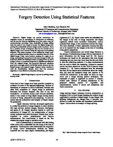
patch-based CNN architecture for the extraction of roads and buildings from high-resolution remotely sensed data. ML-based approaches regard object detection as a classification problem and have achieved significant improvements. ML actively learns from limited training data and can often successfully solve difficult-to-distinguish classification problems [36]. On the other hand, ML usually suffers from insufficient samples and inappropriate features [37]. In order to obtain high-quality results, sample selection and feature extraction need to be studied further. 3. The Proposed Approach 3.1. Overview of the Approach The flowchart of the proposed approach is illustrated in Figure 1. The left part of the flowchart displays the training procedure. The sample database contains all training orthophotos along with corresponding building mask images. Building mask images indicate the exact location and shape of all buildings on an orthophoto. In the segmentation step, the input image is segmented into small homogeneous regions, often called objects or patches. In the candidate selection procedure, some definite non-house objects are eliminated and only candidate objects are left. In the feature extraction step, multiple features are extracted to describe each candidate object. Finally, the classifier model is trained and saved for use in the future. The right part describes the detection (predicting) procedure. Segmentation, candidate selection, and feature extraction are first applied to the test orthophotos. Once the features are generated, the previously trained classifier model is employed to classify the candidate objects into two categories: house and non-house. In the end, the detection results are validated and evaluated.
Figure 1. Flowchart of the proposed approach.
3.2. Image Segmentation This paper employs OBIA to extract objects and the first step is image segmentation. Watershed transformation (WT) is employed to segment the orthophotos due to the efficiency and easy usage of this algorithm [38]. The WT can coincide well with the object edges in the original image, but it usually produces severe over-segmentation results when applied to high-resolution remotely sensed images. To achieve better results, we use a threshold to suppress minor gradient before performing WT, and merge similar adjacent regions using a hierarchical merging algorithm after the WT segmentation. WT suffers from over-segmentation due to a large number of minor gradient values. By carefully tuning, an appropriate threshold Tg = 5 is determined to suppress these minor values. Before WT,
Remote Sens. 2018, 10, 451
6 of 24
the gradient values less than Tg are set to 0. After the initial WT segmentation, a hierarchical merging algorithm begins to merge these regions from finer levels to coarser levels [39]. The merging process continues until no pair of regions can be merged. A threshold Tc is selected to determine whether two adjacent region can be merged. In this paper, Tc is set to 15, at which the algorithm can produce satisfying results. Figure 2 presents an example of the WT segmentation and hierarchical merging result. Figure 2b,c indicate that the segmentation result has been improved after merging and the roofs in the image are well segmented.
Figure 2. Image segmentation based on watershed transformation and hierarchical merging algorithm. (a) Original image; (b) Thresholding watershed segmentation; (c) Results after the hierarchical merging.
3.3. Candidate Selection The selection of candidate regions, which aims to discover potential buildings, can help reduce the search space and simplify the task. As a result of segmentation, the orthophoto is divided into small homogeneous regions, including houses, roads, lawns, trees, and other objects. If all the objects are passed to the next step, it will take a great amount of time to extract features and train the model. It is worth noting that a large number of regions can be definitely determined as non-house objects which will cause imbalanced positive and negative samples if they are not eliminated. Therefore, some domain-specific knowledge is introduced to detect vegetation and shadows [40]. Similar to the studies by Sirmacek et al. [20] and Shorter et al. [41], the color invariance model is used to identify vegetation and shadows. 3.3.1. Vegetation and Shadow Detection Vegetation is a typical landcover and can be relatively easy to identify via the color invariance model originally proposed by Gevers et al. [42]. The color invariance model, defined in Equation (1), is independent of viewpoint, illumination intensity, illumination direction, highlights, and surface orientation. 4 G−B v = · arctan( ). (1) π G+B where G and B are the green and blue channels of the image. The color-invariant image v (Figure 3b) is computed via the green and blue channels from the original orthophoto (Figure 3a) and then Otsu [43] thresholded to obtain a vegetation mask. This process produces a binary image with white pixels corresponding to vegetation candidates and black pixels corresponding to non-vegetation candidates. In remote sensing applications, shadow is one of the major problems that hampers object recognition and change detection (Figure 3a). Shadow detection is still an important research topic, particularly for high-resolution images in urban areas [44]. Among the several shadow detection methods, the color invariance models can be easily used for color aerial images. In our experiments, the following model proposed by Cretu et al. [40] is used to detect shadows.
Remote Sens. 2018, 10, 451
7 of 24
√ I − R2 + G 2 + B2 4 √ s = · arctan( ). π I + R2 + G 2 + B2
(2)
where I is the global intensity of the image, and (R, G, B) are the red, green, and blue components of the given pixel, respectively. After the shadow-invariant image s is computed (Figure 3c), the Ostu thresholding operation is applied to s to produce a binary shadow mask image. Due to the noise in the image, the vegetation and shadow detection results contain a lot of isolated pixels that do not actually correspond to vegetation and shadows. Subsequently, an opening and a closing morphological operation [45] are employed to eliminate these isolated pixels. After these operations, the results can coincide well with the actual boundaries of the vegetation and shadow regions, as shown in Figure 3d.
Figure 3. Candidate selection via vegetation and shadows detection. (a) RGB orthophoto; (b) Colorinvariant image of vegetation; (c) Color-invariant image of shadows; (d) Vegetation and shadow detection results (red areas are shadows and green areas are vegetation); (e) Segmentation results; (f) Candidate regions selected from (e).
3.3.2. Choosing Candidate Regions After the vegetation and shadows are detected, the binary vegetation mask (MaskV ) and the shadow mask (Mask S ) are used together to select the candidates from all the regions produced in the segmentation. Let Regi represent the ith region and A( Regi ) represent the area (number of pixels in the whole region) of this region. Overlapping MaskV and Mask S with the segmented image (Figure 3e), the number of vegetation and shadow pixels located in Regi can be counted and are denoted as
Remote Sens. 2018, 10, 451
8 of 24
A ( Reg )
A ( Reg )
AV ( Regi ) and AS ( Regi ) respectively. If the ratio AV( Reg )i > 0.6 or AS( Reg i) > 0.6, Regi is considered to i i be a non-house object that can be eliminated. After the removal of vegetation and shadow regions, there still exist some tiny regions that are meaningless for further processing and can be removed. Given a predefined area threshold TA , those segmented regions with an area less than TA are eliminated. In this study, a TA of 100 is used. After these processes, all the remaining regions in the segmented image are considered candidates that may be house or non-house objects, as shown in Figure 3f. 3.4. Feature Descriptors for Regions Feature descriptors have a significant impact on the recognition of ground objects. Good features should be non-ambiguous despite changes in angle, illumination, and scale. In classification and object detection, several types of features have been developed, including color features, texture features, and geometric features. In this section, we will present some feature descriptors used in our work as well as some implementation details. 3.4.1. Color Descriptors Color is one of the most common features used to characterize image regions. The images used in our experiments contain only 3 channels; therefore, objects in the images can be distinguished using only red, green, and blue colors. In general, the color feature of a region is represented by the mean color value of all the pixels inside. Due to the variability of color, the mean value cannot fully capture the exact color characteristics. In order to measure the color distribution in an image region, we use color moments to describe the color feature. In our experiments, 1st- and 2nd-order moments are used, as follows: ∑N p ei = j=1 ij . rN (3) N 2 σ = ∑ j=1 ( pij −ei ) . i N where pij is the value of the j-th pixel of the object in the i-th color channel; N is the total number of pixels; ei is the mean value (1st-order moment) in the i-th channel; and σi is the standard deviation (2nd-order moment). In our work, color moments are computed in both RGB and HSV (hue, saturation, and value) color space. In each color channel, two values (ei , σi ) are computed for each object. In both the RGB and HSV color space, we can obtain two 6-dimensional features, denoted as (RGB_mo1 , RGB_mo2 , . . . , RGB_mo6 ) and (HSV_mo1 , HSV_mo2 , . . . , HSV_mo6 ), respectively. 3.4.2. Texture Descriptors Local binary patterns (LBP) was first described by Ojala et al. [46] and has proven to be a powerful feature for texture classification. Due to its discriminative power and computational simplicity, LBP has been seen as a unifying approach to traditional statistical and structural models. The original LBP proceeds as illustrated in Figure 4a: Each pixel value is compared with its neighbors; the neighbors that have greater values than the central pixel are set to bit 1, and others having less or equal values are set to bit 0. One can generate a binary bit serial by concatenating all the bits of the neighbors in a clockwise manner. The binary bits serial is then converted to a decimal LBP code of the central pixel. After processing all the pixels in this way, an LBP map is produced. The histogram calculated over the LBP map image can be used as the descriptor of the original image. Such an LBP defined on 3 × 3 neighbors does not have a good discrimination; therefore, a rotationriu2 , is developed [47]. LBPriu2 is calculated on resampling invariant and uniform LBP, denoted as LBPP,R P,R points along P symmetric directions at a radius of R from the central point. By right-shifting the LBP binary code, one can get different values, of which the minimum is selected as the final LBP code. In
Remote Sens. 2018, 10, 451
9 of 24
Figure 4b, the rotation-invariant uniform LBP map image (middle) is computed on the image of a tree canopy (left) with the parameters of P = 8 and R = 1. The corresponding histogram of the LBP map is shown on the right.
Figure 4. Local binary patterns (LBP) texture. (a) Principle of LBP; (b) LBP texture of the canopy image.
3.4.3. Geometric Descriptors Various types of geometric features have been designed to describe the geometric property of an object. These features can be divided into two categories: simple geometric index and complex shape descriptor. The simple geometric index is a type of feature that can be represented by a single scalar, such as area, circularity, and eccentricity, while the complex shape descriptor is usually described by a vector. This subsection coves some simple geometric indices used in this study. 1.
Area Area is the number of pixels located inside the region boundaries. Here, area is denoted as Ao .
2.
Eccentricity Eccentricity is defined as the ratio of the major axis of a region to its minor axis, described as: Eccentricity = A M /Am .
(4)
where A M and Am are the length of the major axis and that of the minor axis, respectively. 3.
Solidity Solidity describes whether the shape is convex or concave, defined as: Solidity = Ao /Ahull .
(5)
where Ao is the area of the region and Ahull is the convex hull area of the region. 4.
Convexity Convexity is defined as the ratio of the perimeter of the convex hull Phull of the given region over that of the original region Po : Convexity = Phull /Po . (6)
5.
Rectangularity Rectangularity represents how rectangular a region is, which can be used to differentiate circles, rectangles and other irregular shapes. Rectangularity is defined as follows: Rectangularity = As /A R .
(7)
Remote Sens. 2018, 10, 451
10 of 24
where As is the area of the region and A R is the area of the minimum bounding rectangle of the region. The value of rectangularity varies between 0 and 1. 6.
Circularity Circularity, also called compactness, is a measure of similarity to a circle about a region or a polygon. Several definitions are described in different studies, one of which is defined as follows: Circularity = 4πAo /P2 .
(8)
where Ao is the area of the original region and P is the perimeter of the region. 7.
Shape Roughness Shape roughness is a measure of the smoothness of the boundary of a region and is defined as follows: Po Shape_Roughness = . (9) π (1 + ( A M + Am )/2) where Po is the perimeter of the region and A M and Am are the length of the major axis and that of the minor axis, respectively.
3.4.4. Zernike Moments Moment is a typical kind of region-based shape descriptor widely used in object recognition. Among the commonly used region-based descriptors, Zernike moments are a set of excellent shape descriptors based on the theory of orthogonal polynomials [48]. The two-dimensional Zernike moment of order p with repetition q for an image function I (ρ, θ ) in polar coordinates is defined as follows: Z pq =
p+1 ∑ I (ρ, θ )[Vpq (ρ, θ )]∗ , s.t.ρ ≤ 1. π ∑ ρ θ
(10)
where Vpq (ρ, θ ) is a Zernike polynomial that forms a complete orthogonal set over the interior of the unit disc of x2 + y2 ≤ 1. [Vpq (ρ, θ )]∗ is the complex conjugate of Vpq (ρ, θ ). In polar coordinates, Vpq (ρ, θ ) is expressed as follows: Vpq (ρ, θ ) = R pq (ρ)exp(− jqθ ).
(11)
√ where j = −1; p is a non-negative integer; and q is a non-zero integer subject to the constraints that p − |p q| is even and |q| < p; ρ is the length of the vector ρ from the pixel ( x, y) to the origin (0, 0) and ρ = x2 + y2 ; and θ is the angle between the vector ρ and the x axis in a counter clockwise direction. R pq (ρ) is the Zernike radial polynomial defined as follows: ( p−|q|)/2
R pq (ρ) =
∑
s =0
(−1)s ( p − s)! s!(
p+|q| 2
q| − s)!( p−| 2 − s)!
ρ( p−2s) .
(12)
The Zernike moments are only rotation invariant but not scale or translation invariant. To achieve scale and translation invariance, the regular moments, shown as follows, are utilized. m pq =
∑ ∑ x p yq f (x, y).
(13)
Translation invariance is achieved by transforming the original binary image f ( x, y) into a new one f ( x + xo , y + yo ) where (xo , yo ) is the center location of the original image computed by Equation (13) and m00 is the mass (or area) of the image. Scale invariance is accomplished by normalizing the original image into a unit disk, which can be done using xnorm = x/m00 and ynorm = y/m00 . Combing the two points mentioned above, the original image is transformed by Equation (14) before computing
Remote Sens. 2018, 10, 451
11 of 24
Zernike moments. After the transformation, the moments computed upon the image g( x, y) will be scale, translation and rotation invariant. xo = m10 /m00 , yo = m01 /m00 . g( x, y) = f (
x y − xo , − y o ). m00 m00
(14) (15)
3.4.5. Edge Regularity Indices Compared to other objects, parallel and perpendicular lines are more likely to appear around anthropogenic objects such as houses, roads, parking lots, and airports. In order to measure how strongly these lines are perpendicular or parallel to each other, we developed a group of indices called ERI (edge regularity indices) that can describe the spatial relations between these lines. The whole procedure can be divided into two steps. (1) Local Line Segment Detection The first step is local line segment detection, in which line segments are extracted within each candidate region. In general, Hough transformation (HT) is the most common method used to detect line segments. Different from the previous methods, in our work, HT is applied only to each local region instead of the whole image. A local region is defined by the MBR (minimum bounding rectangle) of each segmented region. Figure 5b gives some examples of the MBR of the candidate region in Figure 5a. Before the local HT, a binary edge image is calculated by a Canny edge detection operation (Figure 5c). In the local HT, two parameters are set as follows: HOUG_LEN = 15 and HOUG_GAP = 2. The HOUG_LEN means that only line segments over 15 pixels length are extracted, and HOUG_GAP means that gaps less or equal 2 pixels between two line segments will be filled and that the two segments will be connected. One of the local line segment detection results is shown in Figure 5d; line segments along the house boundaries and on the roofs are detected and delineated in cyan.
Figure 5. Local line segment detection. (a) Candidate regions; (b) Minimum bounding rectangles (MBRs) of the candidate regions; (c) Canny edge detection; (d) Line segments detected by local Hough transformation.
Remote Sens. 2018, 10, 451
12 of 24
(2) Calculation of Indices The second step is to calculate the ERI values. Two scalar values (PerpIdx, ParaIdx) are designed to measure the degree to which these line segments are perpendicular or parallel to each other, and three statistical values (LenMean, LenStd, LenMax) are selected to describe the statistical characteristics of these line segments. (a) PerpIdx is short for perpendicularity index, which describes how strongly the line segments are perpendicular to each other. Take one pair of line segments as an example (Figure 6a). The angle between the two line segments is defined as follows (only the acute angle of the two line segments is considered): |Vi · Vj | Ang(i, j) = arccos( ). (16) |Vi ||Vj | where Vi and Vj are the ith and jth line segments, respectively, which are represented as vectors. For the current local region with n line segments, the total number of these angles can amount to Sumtol = n × (n − 1)/2. If Ang(i, j) ≥ 70 × pi/180, the ith and jth line segments are considered perpendicular to each other. Then, we can sum the number of such approximate right angles as follows: ( CNperp (i, j) =
1, Ang(i, j) > 70 ∗ pi/180. 0, others. n −1
Sum perp =
(17)
n
∑ ∑
CNperp (i, j).
(18)
i =1 j = i +1
The ratio between Sum perp and Sumtol is defined as PerpIdx of the region. PerpIdx =
Sum perp . Sumtol
(19)
Take the line segments in Figure 6b as an example. There are 5 line segments and 6 pairs of line segments that are perpendicular to each other, namely, ( L1 , L3 ), ( L1 , L5 ), ( L2 , L3 ), ( L2 , L5 ), ( L4 , L3 ), and ( L4 , L5 ). The total number of pairs is 5 × 4/2 = 10, and the perpendicularity index is 6/10 = 0.6.
Figure 6. The principle of ERI (edge regularity indices) calculation. (a) Angle between two edges; (b) An example of ERI calculation.
(b) ParaIdx denotes the parallelity index, which is similar to the perpendicularity index but describes how strongly the line segments are parallel to each other. Two line segments are considered
Remote Sens. 2018, 10, 451
13 of 24
parallel to each other only when the angle between them is less than 20 degrees. Thus, the parallelity index of a group of line segments can be computed as follows: ( CNpara (i, j) =
1, Ang(i, j) < 20 ∗ pi/180. 0, others. n −1
Sum para =
(20)
n
∑ ∑
CNpara (i, j).
(21)
Sum para . Sumtol
(22)
i =1 j = i +1
ParaIdx =
For example, Figure 6b contains 4 pairs of parallel line segments: ( L1 , L2 ), ( L1 , L4 ), ( L2 , L4 ), and ( L3 , L5 ); and the parallelity index is 4/10 = 0.4. (c) LenMax, LenMean, and LenStd are the statistics of these line segments. The lengths of all the line segments, denoted as l1 , l2 , ..., lm , are used to calculate the following statistics. LenMean =
∑im=1 (li ) . m
LenStd = std(l1 , l2 , ..., lm ). LenMax = max (l , l , ..., l ). m 1 2
(23)
3.4.6. Shadow Line Indices In most cases, buildings are always accompanied by shadows adjacent to them (Figure 7b). Therefore, the shadow clues represent useful prior knowledge for building detection and are commonly exploited by researchers [23,49]. Different from previous works, we do not directly extract buildings from shadow clues. Instead, we extract shadow line indices (SLI) from shadows and use them in the training process. Furthermore, we found that the edges between a building and its shadow often appear as straight lines. The more numerous and longer straight lines there are in the area adjacent to an object, the more likely the object is to be a building. A feature descriptor that captures the geometric characteristics of shadows can be used to discriminate buildings from other objects. The process of SLI extraction is divided into two steps.
Figure 7. Principle of SLI (shadow line indices) calculation. (a) Detected shadows; (b) Detected line segments at the shadow borders.
The first step is to detect straight line segments along the edges of shadows in the binary mask image (the red pixels in Figure 7a). It should be noted that the edges here are not edges of the whole image but of only shadows, as shown in Figure 7b. After the line segments in each region have been extracted, the SLI can be calculated for these lines. In this study, we select and design 5 scalar values to represent the SLI. Let Li , i = 1, . . . , n denote
Remote Sens. 2018, 10, 451
14 of 24
n line segments. The lengths of these line segments are denoted as l1 , l2 , . . . , ln . The SLI values are computed as follows: ∑n (l ) l_sum = i=n1 i . l_sum l_mean = n . l_std = std(l1 , l2 , . . . , ln ). l_max = max (l1 , l2 , . . . , ln ). l_max l_r = equ_dia .
(24)
where equ_dia is the diameter of a circle with the same area as the current region and l_r represents the ratio between the length of shadow lines and the region size. 3.4.7. Hybrid Descriptors As mentioned above, different features are extracted from each candidate region. Color features in both RGB and HSV color spaces are two 6-dimensional descriptors denoted as RGB_moi , i = 1, . . . , 6 and HSV_moi , i = 1, . . . , 6. The LBP texture with 8 neighbors is used, and the dimension of the LBP descriptor is 8, denoted as LBPi , i = 1, . . . , 8. The Zernike moments are the shape descriptors with the dimension of 25, denoted as Zeri , i = 1, . . . , 25. ERI is a 5-dimensional descriptor and denoted as a vector (PerpIdx, ParaIdx, LenMean, LenStd, LenMax). SLI is a descriptor with 5 dimensions, denoted as: (l_sum, l_mean, l_std, l_max, l_r). Together with other simple geometric indices, including area, eccentricity, solidity, convexity, rectangularity, circularity, and shape roughness, all these descriptors can be concatenated to obtain a long hybrid descriptor, which can enhance the discrimination ability and improve the accuracy of the classification. 3.5. Training and Testing 3.5.1. Labeling and Training After removing vegetation and shadow regions, the remaining regions are either house or non-house (Figure 8a). By manually delineating the exact house footprints in each training orthophoto, we can generate the ground-truth mask map (Figure 8b) in which the white pixels indicate the house position. This mask is then overlapped with the corresponding candidate regions in Figure 8a. The label of each candidate region can be inferred by the size of intersection with the ground-true mask regions. A candidate region for which the intersection with the ground-truth mask exceeds 80% of the area is then labeled as a house (positive sample). After all the positive samples (house regions) are labeled, the remaining candidate regions are labeled as negative samples. As shown in Figure 8c, the positive and negative samples are delineated by red and yellow outlines, respectively. Therefore, in the training process, we need to only manually delineate the house position on the orthophotos, and the positive and negative samples will be automatically generated by the program.
Figure 8. Labeling training samples. (a) Candidate regions; (b) House ROI mask (white = house); (c) Positive (house) and negative (non-house) samples (red = house, yellow = non-house).
Remote Sens. 2018, 10, 451
15 of 24
3.5.2. Testing In the testing process, the input images are processed in the same pipeline. First, the images are preprocessed and segmented using the same algorithms employed in the training process. Then, the vegetation and shadow regions are detected and removed from the initial segmented results. In the next step, features are extracted over each candidate region. Finally, the feature vectors are fed into the classifier trained in the training process to identify houses. 4. Experiments 4.1. Introduction of Data The training dataset used in our experiments consists of about 47 orthophotos from Google Earth in the region of Mississauga City (Figure 9a), which is situated beside Lake Ontario in Canada. Figure 9b presents 9 of these orthophotos, which were acquired in October 2016 and mainly contain residential houses and business buildings. The background includes vegetation, roads, parking lots, vehicles, waters, and other objects. On these training orthophotos, all the houses and buildings have been manually delineated (Figure 9c).
Figure 9. Training data. (a) The location of Mississauga; (b) Training images; (c) Delineated houses.
4.2. Evaluation Metrics There are several possible approaches to evaluate the building detection results. Area- and object- based evaluation are probably the most common approaches to measure the rate of detected buildings. Compared to the area-based method, the object-based method is less sensitive to errors at the building outlines [50]. By overlapping the automatically detected results with the ground-truth map, these regions can be divided into four categories: (1) true positive (TP), house regions that are identified as houses; (2) false positive (FP), non-house regions that are identified as houses; (3) true negative (TN), non-house regions that are identified as non-house; and (4) false negative (FN), house regions that are identified as non-house. In order to calculate TP, FP, TN, and FN, it is necessary to define some rules for judging what type a region in the detected results belongs to. After classification, the regions in the detected results are classified into two types: building and non-building. Let Rb denote a region that is identified as building, and Rn denote a region identified as non-building. If Rb overlaps with one reference building (denoted as R BR ), the percentage of the area of Rb that overlaps with R BR is calculated. If the percentage is no less than Tper , Rb is a TP; if not, it is a FP. In this study, the threshold Tper is set to 60%. According to the same rule, a region Rn can be classified as an FN or a TN. Thus, the numbers of TP, FP, TN, and FN can be calculated and 5 evaluation metrics are computed as follows: ACC PPV TPR TNR
= ( TP + TN )/( TP + FP + TN + FN ). = TP/( TP + FN ). = TP/( TP + FP). = TN/( TP + TN ).
(25)
Remote Sens. 2018, 10, 451
16 of 24
F1_score = p
TP ∗ TN − FP ∗ FN
( TP + FP)( TP + FN )( TN + FP)( TN + FN )
.
(26)
Accuracy (AAC) is the proportion of all predictions that are correct, used to measure how good the model is. Precision (PPV), a measurement of how many positive predictions are correct, is the proportion of positives that are actual positives. Recall (TPR), also called sensitivity or true positive rate, is the proportion of all actual positives that are predicted as positives. Specificity (TNR) is the proportion of actual negatives that are predicted negatives. F1 score can be interpreted as a weighted average of the precision and recall. In order to evaluate the model performance, ROC (receiver operating characteristic) curve is generated by plotting TPR against (1-TNR) at various threshold setting [51]. The closer the curve follows the left-top border, the more accurate the test is. Therefore, the area under the ROC curve (AUC) is used to evaluate how well a classifier performs. 4.3. Results and Quality Assessment In order to test the effectiveness of our approach and those features we selected or designed, we conducted an experiment using three different classifiers, namely AdaBoost, RF (Random Forests), and SVM (Support Vector Machine). The parameters of these classifiers are selected through optimization, as listed in Table 1. The basis estimator of AdaBoost is set as decision tree, and RBF kernel is used in SVM. Table 1. Parameters of classifiers. Classifier
Parameters
Description
AdaBoost
n_max = 90 (optimized) rate = 0.412 (optimized)
The maximum number of estimator at which boosting is terminated. Learning rate.
SVM
Kernel = ‘RBF’ γ = 0.021 (optimized) C = 4.281 (optimized)
Ridial basis function is used as the kernal. γ defines the influence distance of a single example.
RF
n_trees = 45 (optimized) n_sel = 26 (optimized)
Total number of trees in the random forest. The number of tried attributes when splitting nodes.
From the training images, we selected 820 house and building samples. In the test process, we selected another 8 orthophotos (denoted as test01, test02, . . . , test08) in Mississauga. The 8 orthophotos are preprocessed and segmented using the same algorithms employed in the training process. Then features are extracted and fed to the three classifiers to identify the houses. Compared with the ground-truth images, the detection results can be evaluated. Table 2 shows all the evaluation indices of the three classifiers for each test orthophoto. In the table, each line represents the values of these indices, namely accuracy, precision, recall, specificity, F1 score, and AUC. From the table, we can see that the accuracy varies from 77.4% to 92.6%. For object detection missions, we care more about precision and recall rather than accuracy. The best precision, 95.3%, is achieved by RF on test05, and the worst, 73.4%, is achieved by AdaBoost on test03. The highest recall 92.5% is achieved by SVM on test06, and the worst recall is 45.9% achieved by AdaBoost on test08. The last column shows that all AUC values can reach over 86.0% and indicates that all the classifiers perform well in the classification. A classifier does not always perform the best on each of the orthophotos. In order to get an overall evaluation, we average these indices over all the test orthophotos and present the final results in the ’Overall’ rows in Table 2. Among the three classifiers, SVM achieves the best precision (85.2%) and recall (82.5%), while AdaBoost achieves the worst precision (78.7%) and recall (67.1%). Furthermore, the F1 score and AUC also indicate that SVM performs best and that AdaBoost performs the worst. Figure 10 presents the detection results of two of these images, test01 and test08, which are relatively the best and worst results, respectively. Compared with other images, test08 (the second row) contains
Remote Sens. 2018, 10, 451
17 of 24
some contiguous houses and many small sheds. In addition, the roof structures are more complex. As a result, the precision and recall are not as good as that of others. Table 2. Quality evaluation of the results. Method
Data
Acc.
Prec.
Rec.
Spec.
F1 Score
AUC
AdaBoost
test01 test02 test03 test04 test05 test06 test07 test08 Overall
0.889 0.852 0.839 0.833 0.850 0.877 0.774 0.778 0.829
0.811 0.735 0.734 0.831 0.900 0.750 0.792 0.829 0.787
0.896 0.781 0.746 0.673 0.692 0.792 0.514 0.459 0.671
0.885 0.882 0.880 0.923 0.951 0.907 0.923 0.949 0.909
0.851 0.758 0.740 0.744 0.783 0.771 0.623 0.591 0.725
0.951 0.934 0.915 0.918 0.901 0.926 0.870 0.860 0.900
RF
test01 test02 test03 test04 test05 test06 test07 test08 Overall
0.926 0.898 0.905 0.840 0.902 0.911 0.825 0.821 0.872
0.879 0.825 0.855 0.830 0.953 0.807 0.870 0.816 0.848
0.906 0.825 0.803 0.682 0.788 0.868 0.563 0.593 0.731
0.936 0.928 0.945 0.925 0.975 0.927 0.957 0.934 0.938
0.892 0.825 0.828 0.749 0.863 0.836 0.684 0.687 0.785
0.965 0.953 0.948 0.918 0.934 0.950 0.900 0.883 0.926
SVM
test01 test02 test03 test04 test05 test06 test07 test08 Overall
0.926 0.907 0.915 0.873 0.910 0.921 0.901 0.867 0.898
0.903 0.821 0.866 0.854 0.900 0.803 0.868 0.824 0.852
0.875 0.873 0.829 0.766 0.865 0.925 0.831 0.763 0.825
0.952 0.922 0.949 0.930 0.938 0.920 0.936 0.919 0.933
0.889 0.846 0.847 0.808 0.882 0.860 0.849 0.792 0.838
0.966 0.958 0.959 0.947 0.958 0.973 0.939 0.929 0.951
Bold is the highest value in each column and Underline is the lowest.
In order to test how well our model can perform on different orthophotos, we selected another 4 orthophotos containing business buildings. In this experiment, we test only the SVM classifier, which performed the best in the first experiment. Figure 11 presents the detection results. Compared with the manually created ground-truth maps, the evaluation results for each individual image are presented in Table 3, and the last row is the overall evaluation of all the images together. The AUC values indicate that the SVM classifier can still perform well on these images. From the overall evaluation, we can see that the average precision, recall, and F1 score reach 90.2%, 72.4%, and 80.3%, respectively. Table 3. Quality evaluation of the detection results (SVM). Data
Acc.
Prec.
Rec.
Spec.
F1 Score
AUC
test09 test10 test11 test12
0.950 0.867 0.927 0.887
0.875 0.917 0.923 0.886
0.875 0.688 0.750 0.646
0.969 0.966 0.981 0.971
0.875 0.786 0.828 0.747
0.986 0.878 0.915 0.899
Overall
0.910
0.902
0.724
0.973
0.803
0.915
Remote Sens. 2018, 10, 451
18 of 24
Figure 10. House detection results on image test1 (first row) and test8 (second row). (a) Original images; (b) Results of AdaBoost; (c) Results of Random Forest (RF); (d) Results of Support Vector Machine (SVM).
Figure 11. Results of building Detection. (a) Test09; (b) Test10; (c) Test11; (d) Test12.
4.4. Evaluation of Different Features In this experiment, we will evaluate the contribution of each type of features in the house detection task. We can group all the features into 5 categories: (1) Color features: RGB_moi , i = 1, . . . , 6 and HSV_moi , i = 1, . . . , 6; (2) LBP texture: LBPi , i = 1, . . . , 8; (3) Zernike moments: Zeri , i = 1, . . . , 25; (4) ERI + SLI: (PerpIdx, ParaIdx, LenMean, LenStd, LenMax) and (l_sum, l_mean, l_std, l_max, and l_r); and (5) Geometric indices: area, eccentricity, solidity, convexity, rectangularity, circularity and shape roughness. Random forest is employed in this experiment because RF can provide the
Remote Sens. 2018, 10, 451
19 of 24
importance value of each feature during the training. This can help evaluate how much one feature contribute to the classification. We performed the RF training procedure 10 times and calculate the mean importance value for each group feature mentioned above, presenting the result in Table 4. The result shows that ‘ERI + SLI’ has the highest importance, and ‘Geometric indices’ and ‘Zernike moments’ follow with nearly the same importance. The above evaluation just indicates the importance of each group feature in the training procedure. In order to further test the performance of each group feature, we employ each group feature alone to detect houses from the test images (test09–test12). Each time, only one group of features is selected to train and test. Besides the 5 groups of features mentioned above, we also use 2 groups of combined features. One is the whole combination of all features, denoted as ‘All’, and the other is the all combination except ERI and SLI, denoted as ‘All-(ERI + SLI)’. Figure 12 shows the detection results produced by different feature groups, and the quality assessment results are presented in Table 5. The classification accuracy of all the feature groups can reach over 76.6% and the AUC can reach over 74.7%. For object detection, precision, recall, and F1 Score are more indicative than other quality assessment indices. Among the 5 individual feature groups, ‘ERI + SLI’ achieves the highest precision 87.6% and the highest recall 55.5%; ‘ERI + SLI’ achieves the highest F1 score 67.0% and ’Geometric indices’ follows with a value of 63.8%. Overall, our proposed features ‘SLI + ERI’ outperform the other features Color, LBP texture, Zernike moments and Geometric indices, when employed alone. Furthermore, the first two rows of Table 5 show that our proposed features ‘ERI + SLI’ can help improve the quality of detection results. ‘All-(ERI + SLI)’ means that all other features except ERI and SLI are used in the experiment, and ‘All’ means that all features including ERI and SLI are used. Comparing the two rows, we can see that the precision, recall and F1 score increase by 5.6%, 11.2% and 9.0%, respectively, when the ERI and SLI are used together with other features. The evaluation results indicate that the proposed features are effective for house detection. Table 4. Importance of features. Features
Color
LBP
Geometric Indices
Zernike Moments
ERI + SLI
Sum.
Importance
0.1269
0.1845
0.2030
0.2011
0.2845
1.0000
Table 5. Evaluation of features. Features
Acc.
Prec.
Rec.
Spec.
F1 Score
AUC
all All-(ERI + SLI)
0.905 0.861
0.896 0.840
0.765 0.653
0.961 0.947
0.825 0.735
0.935 0.903
ERI + SLI Color LBP Geo Zer
0.841 0.771 0.767 0.825 0.766
0.876 0.642 0.666 0.825 0.713
0.555 0.432 0.452 0.527 0.374
0.954 0.896 0.887 0.945 0.923
0.670 0.486 0.520 0.638 0.480
0.875 0.793 0.789 0.848 0.747
Remote Sens. 2018, 10, 451
20 of 24
Figure 12. Building detection results using different features. (a) All features; (b) All-(edge regularity indices (ERI) + shadow line indices (SLI)); (c) ERI + SLI; (d) Color; (e) local binary patterns (LBP); (f) Geometric indices; (g) Zernike moments.
4.5. Discussion We utilized 3 machine learning methods, namely, AdaBoost, RF, and SVM, to test our approach. As shown in Table 2, all the classifiers can obtain an overall accuracy from 82.9% to 89.8% and an overall AUC from 86.0% to 97.3%, and the results indicate that our approach performs well for house detection. The precision and the recall are commonly used to measure how well the method can identify the objects. Overall, the precision values of AdaBoost, RF, and SVM can reach 78.7%, 84.8%, and 85.2%, respectively; and the recall values of the three classifiers can reach 67.1%, 73.1%, and 82.5%, respectively. Combined with SVM, the proposed approach can achieve the best precision of 85.2% and the best recall of 82.5%. The evaluations show that our proposed ERI and SLI features perform well on house detection, achieving the highest score among the 5 individual feature groups. When combined with other features, the ERI and SLI can improve the precision, recall, and F1 score by 5.6%, 11.2%, and 9.0%, respectively.
Remote Sens. 2018, 10, 451
21 of 24
From the detection results (Figure 12), we can see that color, texture features cannot distinguish roads from buildings. Geometric and shadow clues can help discriminate objects having the similar spectral characteristics and thus improve the precision. The precision of identification is also impacted by the image segmentation, which is crucial for object-based image analysis. In our experiments, the segmentation results are still far from being perfect and unavoidably results in inaccurate detection. From Figures 10–12, we can see that some roofs are not delineated as a whole due to the inaccurate segmentation. 5. Conclusions In this paper, we propose an OBIA and machine learning based approach for detecting houses from RGB high-resolution images. The proposed approach shows the ability of machine learning in object detection domain, which is proven by the results of experiments and evaluations. In order to capture geometric features and exploit spatial relations, we propose two new feature descriptors, namely, ERI (edge regularity indices) and SLI (shadow line indices), which help to discriminate houses from other objects. Evaluation results show that the two combined features ‘ERI + SLI’ outperform other commonly used features when employed alone in house detection. Further evaluations show that ‘ERI + SLI’ features can increase the precision and recall of the detection results by about 5.6% and 11.2%, respectively. The approach has several advantages that make it valuable and applicable in automatic object detection from remotely sensed images. First, the whole process, from inputting training data to generating output results, is fully automatic, meaning that no interaction is needed. Certainly, some parameters should be predefined before executing the programs. Second, the proposed method needs only RGB images without any other auxiliary data that sometimes are not easy to obtain. Without limitations from the data source, this approach is valuable in practical applications. Third, this approach has low requirements for training data. In our experiments, 47 Google Earth image patches containing about 820 house samples are selected to train the model, implying that it is easy to collect sufficient training data. This approach is mainly tested on detecting residential houses and business buildings in suburban areas, and it is effective and applicable. The approach can also be extended to house mapping or rapid assessment of house damage caused by earthquakes in suburban or rural areas. Although this study indicates that the proposed approach is effective for house identification, further exploration is still required. The image segmentation algorithm tends to segment a whole roof into separate segments due to variable illumination. Therefore, more robust and reliable algorithms should be developed to improve the segmentation results. In the experiments, we found that some roads and concrete areas are still misclassified as house roofs because current features are not powerful enough to discriminate one from another. Therefore, more powerful and reliable features need to be explored further. To test the approach’s stability, some more extended and sophisticated areas, for example high-density building urban areas, need to be tested. Acknowledgments: The research is supported by the National Natural Science Foundation of China (No. 41471276). The authors would also like to thank the editors and the anonymous reviewers for their comments and suggestions. Author Contributions: Renxi Chen conceived the idea, designed the flow of the experiments, and implemented the programs. In addition, he wrote the paper. Xinhui Li prepared the data sets, conducted the experiments, and analyzed the results. Jonathan Li provided some advice and suggested improvements in writing style and its structure. Conflicts of Interest: The authors declare no conflict of interest.
Remote Sens. 2018, 10, 451
22 of 24
Abbreviations The following abbreviations are used in this manuscript: AdaBoost AUC CNN DSM ERI GIS HMT HT LBP ML OBIA RF RGB ROC SLI SVM VHR WT
adaptive boost area under the curve convolutional neural network digital surface model edge regularity indices geographic information systems hit-or-miss transformation Hough transformation local binary patterns machine learning object-based image analysis random forests red, green, and blue receiver operating characteristic shadow line indices support vector machine very high resolution watershed transformation
References 1.
2. 3.
4. 5. 6. 7. 8. 9. 10.
11. 12.
13.
Quang, N.T.; Thuy, N.T.; Sang, D.V.; Binh, H.T.T. An efficient framework for pixel-wise building segmentation from aerial images. In Proceedings of the 6th International Symposium on Information and Communication Technology, Hue City, Viet Nam, 3–4 December 2015; pp. 282–287. Li, E.; Xu, S.; Meng, W.; Zhang, X. Building extraction from remotely sensed images by integrating saliency cue. IEEE J. Sel. Top. Appl. Earth Obs. Remote Sens. 2017, 10, 906–919. Lin, C.; Huertas, A.; Nevatia, R. Detection of buildings using perceptual grouping and shadows. In Proceedings of the IEEE Conference on Computer Vision and Pattern Recognition, Seattle, WA, USA, 21–23 June 1994; pp. 62–69. Katartzis, A.; Sahli, H. A stochastic framework for the identification of building rooftops using a single remote sensing image. IEEE Trans. Geosci. Remote Sens. 2008, 46, 259–271. Kim, T.; Muller, J.P. Development of a graph-based approach for building detection. Image Vis. Comput. 1999, 17, 3–14. San, D.K.; Turker, M. Building extraction from high resolution satellite images using Hough transform. Int. Arch. Photogramm. Remote Sens. Spat. Inf. Sci. 2010, XXXVIII, 1063–1068. Cheng, G.; Han, J. A survey on object detection in optical remote sensing images. ISPRS J. Photogramm. Remote Sens. 2016, 117, 11–28. Lefèvre, S.; Weber, J. Automatic building extraction in VHR images using advanced morphological operators. In Proceedings of the IEEE Urban Remote Sensing Joint Event, Paris, France , 11–13 April 2007; pp. 1–5. Stankov, K.; He, D.C. Building detection in very high spatial resolution multispectral images using the hit-or-miss transform. IEEE Geosci. Remote Sens. Lett. 2013, 10, 86–90. Stankov, K.; He, D.C. Detection of buildings in multispectral very high spatial resolution images using the percentage occupancy hit-or-miss transform. IEEE J. Sel. Top. Appl. Earth Obs. Remote Sens. 2014, 7, 4069–4080. Peng, J.; Zhang, D.; Liu, Y. An improved snake model for building detection from urban aerial images. Pattern Recognit. Lett. 2005, 26, 587–595. Ahmadi, S.; Zoej, M.J.V.; Ebadi, H.; Abrishami, H.; Mohammadzadeh, A. Automatic urban building boundary extraction from high resolution aerial images using an innovative model of active contours. Int. J. Appl. Earth Obs. Geoinf. 2010, 12, 150–157. Yari, D.; Mokhtarzade, M.; Ebadi, H.; Ahmadi, S. Automatic reconstruction of regular buildings using a shape-based balloon snake model. Photogramm. Rec. 2014, 29, 187–205.
Remote Sens. 2018, 10, 451
14.
15. 16.
17. 18. 19. 20.
21. 22.
23. 24.
25.
26. 27. 28. 29. 30. 31.
32. 33. 34.
35. 36.
23 of 24
Blaschke, T.; Hay, G.J.; Kelly, M.; Lang, S.; Hofmann, P.; Addink, E.; Queiroz Feitosa, R.; van der Meer, F.; van der Werff, H.; van Coillie, F.; Tiede, D. Geographic object-based image analysis—Towards a new paradigm. ISPRS J. Photogramm. Remote Sens. 2014, 87, 180–191. Ziaei, Z.; Pradhan, B.; Mansor, S.B. A rule-based parameter aided with object-based classification approach for extraction of building and roads from WorldView-2 images. Geocarto Int. 2014, 29, 554–569. Grinias, I.; Panagiotakis, C.; Tziritas, G. MRF-based segmentation and unsupervised classification for building and road detection in peri-urban areas of high-resolution satellite images. ISPRS J. Photogramm. Remote Sens. 2016, 122, 145–166. Huertas, A.; Nevatia, R. Detecting buildings in aerial images. Comput. Vis. Graph. Image Process. 1988, 41, 131–152. Irvin, R.B.; McKeown, D.M. Methods for exploiting the relationship between buildings and their shadows in aerial imagery. IEEE Trans. Syst. Man Cybern. 1989, 19, 1564–1575. Liow, Y.T.; Pavlidis, T. Use of shadows for extracting buildings in aerial images. Comput. Vis. Graph. Image Process. 1990, 49, 242–277. Sirmacek, B.; Unsalan, C. Building detection from aerial images using invariant color features and shadow information. In Proceedings of the 23rd International Symposium on Computer and Information Sciences, ISCIS 2008, Istanbul, Turkey , 27–29 October 2008; pp. 105–110. Huang, X.; Zhang, L. Morphological building/shadow index for building extraction from high-resolution imagery over urban areas. IEEE J. Sel. Top. Appl. Earth Obs. Remote Sens. 2012, 5, 161–172. Benarchid, O.; Raissouni, N.; Adib, S.E.; Abbous, A.; Azyat, A.; Ben, A.N.; Lahraoua, M.; Chahboun, A. Building extraction using object-based classification and shadow information in very high resolution multispectral images, a case study: Tetuan, Morocco. Can. J. Image Process. Comput. Vis. 2013, 4, 1–8. Chen, D.; Shang, S.; Wu, C. Shadow-based building detection and segmentation in high-resolution remote sensing image. J. Multimedia 2014, 9, 181–188. Durieux, L.; Lagabrielle, E.; Nelson, A. A method for monitoring building construction in urban sprawl areas using object-based analysis of Spot 5 images and existing GIS data. ISPRS J. Photogramm. Remote Sens. 2008, 63, 399–408. Sahar, L.; Muthukumar, S.; French, S.P. Using aerial imagery and GIS in automated building footprint extraction and shape recognition for earthquake risk assessment of urban inventories. IEEE Trans. Geosci. Remote Sens. 2010, 48, 3511–3520. Guo, Z.; Du, S. Mining parameter information for building extraction and change detection with very high-resolution imagery and GIS data. GISci. Remote Sens. 2017, 54, 38–63. Sohn, G.; Dowman, I. Data fusion of high-resolution satellite imagery and LiDAR data for automatic building extraction. ISPRS J. Photogramm. Remote Sens. 2007, 62, 43–63. Hermosilla, T.; Ruiz, L.A.; Recio, J.A.; Estornell, J. Evaluation of automatic building detection approachs combining high resolution images and LiDAR data. Remote Sens. 2011, 3, 1188–1210. Partovi, T.; Bahmanyar, R.; Krauß, T.; Reinartz, P. Building outline extraction using a heuristic approach based on generalization of line segments. IEEE J. Sel. Top. Appl. Earth Obs. Remote Sens. 2017, 10, 933–947. Chai, D. A probabilistic framework for building extraction from airborne color image and DSM. IEEE J. Sel. Top. Appl. Earth Obs. Remote Sens. 2017, 10, 948–959. Vakalopoulou, M.; Karantzalos, K.; Komodakis, N.; Paragios, N. Building detection in very high resolution multispectral data with deep learning features. In Proceedings of the IEEE International Geoscience and Remote Sensing Symposium, Milan, Italy, 26–31 July 2015, pp. 1873–1876. Guo, Z.; Shao, X.; Xu, Y.; Miyazaki, H.; Ohira, W.; Shibasaki, R. Identification of village building via Google Earth images and supervised machine learning methods. Remote Sens. 2016, 8, 271. Cohen, J.P.; Ding, W.; Kuhlman, C.; Chen, A.; Di, L. Rapid building detection using machine learning. Appl. Intell. 2016, 45, 443–457. Dornaika, F.; Moujahid, A.; Merabet, Y.E.; Ruichek, Y. Building detection from orthophotos using a machine learning approach: An empirical study on image segmentation and descriptors. Expert Syst. Appl. 2016, 58, 130–142. Alshehhi, R.; Marpu, P.R.; Woon, W.L.; Mura, M.D. Simultaneous extraction of roads and buildings in remote sensing imagery with convolutional neural networks. ISPRS J. Photogramm. Remote Sens. 2017, 130, 139–149. Pal, M. Random forest classifier for remote sensing classification. Int. J. Remote Sens. 2005, 26, 217–222.
Remote Sens. 2018, 10, 451
37. 38. 39. 40.
41. 42. 43. 44. 45. 46. 47. 48. 49. 50. 51.
24 of 24
Yuan, J.; Cheriyadat, A.M. Learning to count buildings in diverse aerial scenes. In Proceedings of the International Conference on Advances in Geographic Information Systems, Dallas, TX, USA, 4–7 November 2014. Roerdink, J.B.; Meijster, A. The watershed transform: Definitions,algorithms and parallelization strategies. Fundam. Inform. 2000, 41, 187–228. Haris, K.; Efstratiadis, S.N.; Maglaveras, N.; Katsaggelos, A.K. Hybrid image segmentation using watersheds and fast region merging. IEEE Trans. Image Process. 1998, 7, 1684–1699. Cretu, A.M.; Payeur, P. Building detection in aerial images based on watershed and visual attention feature descriptors. In Proceedings of the International Conference on Computer and Robot Vision, Regina, SK, Canada, 28–31 May 2013; pp. 265–272. Shorter, N.; Kasparis, T. Automatic vegetation identification and building detection. Remote Sens. 2009, 1, 731–757. Gevers, T.; Smeulders, A.W.M. PicToSeek: Combining color and shape invariant features for image retrieval. IEEE Trans. Image Process. 2000, 9, 102–119. Otsu, N. A threshold selection method from gray-level histograms. IEEE Trans. Syst. Man Cybern. 1979, 9, 62–66. Shahtahmassebi, A.; Yang, N.; Wang, K.; Moore, N.; Shen, Z. Review of shadow detection and de-shadowing methods in remote sensing. Chin. Geogr. Sci. 2013, 23, 403–420. Breen, E.J.; Jones, R.; Talbot, H. Mathematical morphology: A useful set of tools for image analysis. Stat. Comput. 2000, 10, 105–120. Ojala, T.; Pietikainen, M.; Harwood, D. A comparative study of texture measures with classification based on feature distributions. Pattern Recognit. 1996, 29, 51–59. Ojala, T.; Pietikainen, M.; Maenpaa, T. Multiresolution gray-scale and rotation invariant texture classification with Local Binary Pattern. IEEE Trans. Pattern Anal. Mach. Intell. 2002, 24, 971–987. Teague, M.R. Image Analysis via the general theory of moments. J. Opt. Soc. Am. 1980, 70, 920–930. Singh, G.; Jouppi, M.; Zhang, Z.; Zakhor, A. Shadow based building extraction from single satellite image. Proc. SPIE Comput. Imaging XIII 2015, 9401, 94010F. Potuckova, M.; Hofman, P. Comparison of quality measures for building outline extraction. Photogramm. Rec. 2016, 31, 193–209. Powers, D. Evaluation: From Precision, Recall and F-Measure to ROC, Informedness, Markedness & Correlation. J. Mach. Learn. Technol. 2011, 2, 37–63. c 2018 by the authors. Licensee MDPI, Basel, Switzerland. This article is an open access
article distributed under the terms and conditions of the Creative Commons Attribution (CC BY) license (http://creativecommons.org/licenses/by/4.0/).