Abstractâ Cognitive networks enable efficient sharing of the radio spectrum. Control signals used to setup a communication are broadcast to the neighbors in ...
Selective Broadcasting in Multi-Hop Cognitive Radio Networks Yogesh R Kondareddy and Prathima Agrawal Department of Electrical and Computer Engineering Auburn University, Auburn, AL 36849 E-mail: {kondayr, agrawpr}@auburn.edu
Abstract— Cognitive networks enable efficient sharing of the radio spectrum. Control signals used to setup a communication are broadcast to the neighbors in their respective channels of operation. But since the number of channels in a cognitive network is potentially large, broadcasting control information over all channels will cause a large delay in setting up the communication. Thus, exchanging control information is a critical issue in cognitive radio networks. This paper deals with selective broadcasting in multi-hop cognitive radio networks in which, control information is transmitted over pre-selected set of channels. We introduce the concept of neighbor graphs and minimal neighbor graphs to derive the essential set of channels for transmission. It is shown through simulations that selective broadcasting reduces the delay in disseminating control information and yet assures successful transmission of information to all its neighbors. It is also demonstrated that selective broadcasting reduces redundancy in control information and hence reduces network traffic. Keywords- Cognitive Network, neighbor graph, minimal neighbor graph, selective broadcast, complete broadcast.
I. INTRODUCTION The idea of cognitive networks was introduced to increase the efficiency of spectrum utilization. The basic idea of cognitive networks is to permit other users to utilize the spectrum allocated to licensed users (primary users) when it is not being used by them. These other users who are opportunistic users of the spectrum are called secondary users. Cognitive radio [1] technology enables secondary users to dynamically sense the spectrum for spectrum holes and utilize the same for their communication. A group of such independent, cognitive users communicating with each other in a multi-hop fashion form a multi-hop cognitive radio network (MHCRN). Each cognitive user (secondary user) will be referred to as a ‘node’ in the rest of the paper. Since the unused spectrum is shared among a group of independent users, there should be a way to control and coordinate access to the spectrum. This can be achieved using a centralized control or by a cooperative distributed approach. In a centralized architecture, a single entity, called spectrum administrator, controls the usage of the spectrum by secondary users [2]. The spectrum administrator gathers the information about free channels either by sensing its entire domain or by integrating the information collected by potential secondary users in their respective local areas. These users send information to the spectrum administrator through a dedicated
control channel. This approach is not feasible for dynamic multi-hop networks. Moreover, a direct attack such as a Denial of Service attack (DoS) [3] on the spectrum administrator would incapacitate the network. Thus, a distributed approach is preferred over a centralized control. In a distributed approach, there is no central administrator. As a result, all users should cooperatively sense and share the free channels. The information sensed by a user should be shared with other users in the network to enable certain essential tasks like route discovery in a MHCRN. Such control information is broadcast to its neighbors in a traditional network. Since in a cognitive network, each node has a set of channels available, a node receives a message only if the message was sent in the channel on which the node was listening to. So, to ensure that a message is successfully sent to all neighbors of a node, it has to be broadcast in every channel. This is called complete broadcasting of information. In a cognitive environment, the number of channels is potentially large. As a result broadcasting in every channel causes a large delay in transmitting the control information. Another solution would be to choose one channel from among the free channels for control signal exchange. However, the probability that a channel is common with all the cognitive users is small [4]. As a result, some of the nodes may not be reachable using a single channel. So, it is necessary to broadcast the control information on more than one channel to ensure that every neighbor receives a copy [5]. With the increase in number of nodes in the network, it is possible that the nodes are scattered over a large set of channels. As a result, cost and delay of broadcasting over all these channels increases. A simple, yet efficient solution would be to identify a small subset of channels which cover all the neighbors of a node. Then use this set of channels for exchanging the control information. This concept of transmitting the control signals over a selected group of channels instead of flooding over all channels is called selective broadcasting and forms the basic idea of the paper. Neighbor graphs and minimal neighbor graphs are introduced to find the minimal set of channels to transmit the control signals. The rest of the paper is organized as follows: Section II describes selective broadcasting. Section III introduces neighbor graphs and minimal neighbor graphs. In Section IV the advantages of selective broadcasting are discussed. Section V presents simulation results and section VI concludes the paper.
II. SELECTIVE BROADCASTING In a MHCRN, each node has a set of channels available when it enters a network. In order to become a part of the network and start communicating with other nodes, it has to first know its neighbors and their channel information. Also, it has to let other nodes know its presence and its available channel information. So it broadcasts such information over all channels to make sure that all neighbors receive the message. Similarly, when a node wants to start a communication it should exchange certain control information useful, for example, in route discovery. However, a cognitive network environment is dynamic due to the primary user’s traffic [6]. The number of available channels at each node keeps changing with time and location. To keep all nodes updated, the information change has to be transmitted over all channels as quickly as possible. So, for effective and efficient coordination, fast dissemination of control traffic between neighboring users is required. So, minimal delay is a critical factor in promptly disseminating control information. Hence, the goal is to reduce the broadcast delay of each node.
III.
NEIGHBOR GRAPH AND MINIMAL NEIGHBOR GRAPH FORMATION
In this section, the idea of neighbor graph and minimal neighbor graph is introduced and the construction of the same is explained. A neighbor graph of a node represents its neighbors and the channels over which they can communicate. A minimal neighbor graph of a node represents its neighbors and the minimum set of channels through which it can reach all its neighbors. The detailed construction of both such graphs is explained below. A. Construction of neighbor graph Each node maintains a neighbor graph. In a neighbor graph, each user is represented as a node in the graph. Each channel is represented by an edge. Let graph G denote the neighbor graph, with N and C representing the set of nodes and all possible channels, respectively. An edge is added between a pair of nodes if they can communicate through a channel. So a pair of nodes can have 2 edges if they can use two different frequencies (channels). For example, if nodes A and B have two channels to communicate, then it is represented as shown in Fig. 1a. A and B can communicate through channels 1 and 2. Therefore, nodes A and B are connected by two edges.
Now, consider that a node has M available channels. Let Tb be the minimum time required to broadcast a control message. Then, total broadcast delay = M × T b So, in order to have lower broadcast delay we need to reduce M . The value of Tb is dictated by the particular hardware used and hence is fixed. M can be reduced by finding the minimum number of channels, M ' to broadcast, but still making sure that all nodes receive the message. Thus, broadcasting over carefully selected M ' channels instead of blindly broadcasting over M (available) channels is called Selective Broadcasting. Finding the minimum number of channels M ' is accomplished by using neighbor graphs and finding out the minimal neighbor graphs.
Figure 1. a) Nodes A and B linked by 2 edges. b) Representation of node A with 6 neighbors
Before explaining the idea of neighbor graph and minimal neighbor graph it is important to understand the state of the network when selective broadcasting occurs and the difference between multicasting and selective broadcasting.
Now, consider a graph with 7 nodes and 4 different channels as shown in Fig. 1b. Node A is considered the source node. It has 6 neighbors, B through G. The edges represent the channels through which A can communicate with its neighbors. For example, A and D can communicate through channels 1 and 2. It means that they are neighbors to each other in channels 1 and 2. This graph is called the neighbor graph of node A. Similarly every node maintains its neighbor graph.
State of the network: When a node enters the network for the first time, it has no information about its neighbors. So, initially, it has to broadcast over all the possible channels to reach its neighbors. This is called the initial state of the network. From then on, it can start broadcasting selectively. Network steady state is reached when all nodes know their neighbors and their channel information. Since selective broadcasting starts in the steady state, all nodes are assumed to be in steady state during the rest of the discussion. Multicasting and Selective broadcasting: Broadcasting is the nature of wireless communication. As a result, Multicasting and Selective broadcasting might appear similar, but they differ in basic idea itself. Multicasting is used to send a message to a specific group of nodes in a particular channel. In a multichannel environment where the nodes are listening to different channels, Selective broadcasting is an efficient way to broadcast a message to all its neighbors. It uses a selected set of channels to broadcast the information instead of broadcasting in all the channels.
B. Construction of Minimal Neighbor graph To reduce the number of broadcasts, the minimum number of channels through which a node can reach all its neighbors has to be chosen. A minimal neighbor graph represents such a set of channels. Let DC be a set whose elements represent the degree of each channel in the neighbor graph. So, DCi represents the number of edges corresponding to channel Ci . For example, the set DC of the graph in Fig. 1b is: DC = {3,3,1, 2} . To build the minimal neighbor graph, the channel with the highest degree in DC is chosen. All edges corresponding to this channel, as well as all nodes other than the source node that are connected to these edges in the neighbor graph, are removed. This channel is added to a set
2
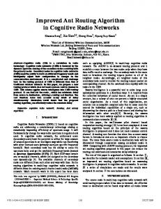
Figure 2. Stepwise development of minimal neighbor graph and the Essential Channel Set (ECS)
called ‘Essential Channel Set’, ECS which as the name implies, is the set of required channels to reach all the neighboring nodes. ECS initially is a null set. As the edges are removed, the corresponding channel is added to ECS .
3) Construct DC from the neighbor graph obtained above. 4) Set ECS to NULL. 5) Remove the edges corresponding to the channel which has the highest degree in DC . 6) Remove the nodes attached to the removed edges, leaving the main node intact. 7) Update sets DC and ECS . 8) Check if the node left is the main node. If no, go to step 5. 9) Build the minimal neighbor graph, by removing all the edges from the original neighbor graph, which do not correspond to the channels in ECS .
For example, reconsider the neighbor graph shown in Fig. 1b. The step wise formation of a minimal neighbor graph and the ECS for this example is illustrated in Fig. 2. Initially, ECS is set to null. Since channel 1 has the highest degree in DC , the edges corresponding to channel 1 are removed in the first step. Also, nodes B, C and D are removed from the graph and channel 1 is added to ECS . It can be seen that sets DC and ECS are updated for the next step. This process continues until only the source node is left. At this point ECS contains all the essential channels. The minimal neighbor graph is formed by removing all the edges from the original neighbor graph, which do not correspond to the channels in ECS . The final minimal neighbor graph is shown in Fig. 3. Since, ECS is constructed by adding only the required channels from C ; ECS is a subset of C .
IV. ADVANTAGE OF SELECTIVE BROADCASTING In this section the advantages of selective broadcasting when compared to complete broadcasting are discussed. A. Broadcast delay It was shown in section II that broadcast delay is reduced if M ' < M , where M is the number of available channels at a node and M ' is the number of minimum channels required to reach all its neighbors. Since C is the channel set of all available channels and ECS is the channel set of minimum channels,
M = Cardinality of C M ' = Cardinality of ECS But, it was shown that ECS is a subset of C . Therefore, Figure 3. Final minimal neighbor graph of fig. 1b.
M '≤ M
Algorithm 1, shown below is used for the construction of the Neighbor graph and the Minimal Neighbor graph.
Since it is shown that the number of channels over which to transmit in selective broadcasting is less than that in complete broadcasting, the broadcast delay is reduced.
Algorithm 1 Construction of Minimal Neighbor graph.
B. Less congestion, contention Since in selective broadcasting, the average number of broadcasts per channel is reduced, the overall congestion in the network is reduced. Moreover, when the traffic in the network increases, the total number of broadcast messages also increases. As a result, there is increased contention in every channel. But using selective broadcasting, traffic is reduced compared to complete broadcasting which leads to lower contention. This implies that a potential improvement in the
1) Add a node N i to the graph G for each user in MHCRN. 2) Add an edge between node N i and node N j if they are neighbors through channel Ci for all N i , N j ∈ N and
Ci ∈ C . Graph G is called the Neighbor graph.
3
overall network throughput can be achieved by using selective broadcasting. C. No common control channel Many MAC protocols have been proposed which assume common channel for control message transmission [6]. But the use of common control channel introduces some problems such as channel saturation and Denial of Service attacks (DoS) [3]. Selective broadcasting, in addition to the above mentioned advantages, is free from DoS attack. It is due to the fact that it inherently avoids the necessity of common control channel. Absence of common control channel also results in significant increase in throughput as shown in [7].
Figure 5. Plot of node density per channel with respect to number of channels for a set of 50 nodes
In the following section, the effectiveness of the proposed concept is demonstrated using simulations. V.
A. Broadcast Delay In this part of the simulations, transmission delay of selective broadcast and complete broadcast are compared. Broadcast delay is defined as the total time taken by a node to successfully transmit one control message to all its neighbors. Each point in the following graphs is the average delay of all nodes in the network. The minimum time to broadcast in a channel is assumed to be 5 msec.
SIMULATION RESULTS
In this section the performance selective broadcast is compared with complete broadcasting by studying the delay in transmitting control information and redundancy of the received packets. The simulation setup used in all these experiments is shown below. Simulation setup
Fig. 6 shows the average delay with respect to the number of nodes. It can be observed that in selective broadcasting the delay in disseminating the control information to all neighbors of a node is much less than that for complete broadcast. In selective broadcasting, the delay increases with the number of nodes because, with increase in the number of nodes, the nodes are spread over increased number of channels as demonstrated in observation 1. As a result, a node might have to transmit over more number of channels. In complete broadcasting, a node transmits over all its available channels. Since the channels are assigned randomly to the nodes, the average number of channels at each node is almost constant. Therefore the delay is constant as observed in Fig. 6.
MATLAB has been used for all simulations. For each experiment, a network area of 1000m×1000m is considered. The number of nodes is varied from 1 to 100. All nodes are deployed randomly in the network. Each node is assigned a random set of channels varying from 0 to 10 channels. The transmission range is set to 250m. Each data point in the graphs is an average of 100 runs. Before looking at the performance of the proposed idea, two observations are made that help in understanding the simulation results. Fig. 4 shows the plot of channel spread as a function of number of nodes. Channel spread is defined as the union of all the channels covered by the neighbors of a node. Observation 1: With increase in number of nodes, the neighbors of a node are spread over larger number of channels.
Figure 6. Comparison of average broadcast delay of a node as number of nodes is varied.
Fig. 7 shows the average delay as a function of the number of channels in a network of 50 nodes. As can be expected, the average delay increases linearly with increase in the number of channels in the case of complete broadcast, because the node transmits in all its available channels. On the other hand, in selective broadcasting, the rate of increase in average delay is very small. This is because, with increase in the number of channels, the number of neighboring nodes covered by each channel also increases as demonstrated in observation 2. As a
Figure 4. Plot of channel spread with respect to number of nodes for a set of 10 channels.
Fig. 5 shows the plot of node density per channel as a function of number of channels. Node density per channel is the number of neighbors covered by a channel. Observation 2: With increase in number of channels, the number of neighbors each channel covers increases.
4
result, the minimum channel set required to cover all the neighbors remains nearly constant inturn keeping the delay constant.
Figure 9. Comparison of average redundancy of messages at a node as number of channels is varied.
In this section, it has been demonstrated that selective broadcasting provides lower transmission delay and redundancy. It should be noted that, due to the reduced redundancy of messages, there will be less congestion in the network and hence, there is potential for improvement in throughput by using selective broadcasting.
Figure 7. Comparison of average broadcast delay of a node as number of channels is varied.
B. Redundancy ‘Redundancy’ in this context is defined as the total number of extra copies of a message received by all nodes in the network if all of them transmit control messages once.
VI.
CONCLUSION
In this paper a new concept of selective broadcasting in MHCRNs is introduced. A minimum set of channels called the Essential Channel Set (ECS), is derived using neighbor graph and minimal neighbor graph. This set contains the minimum number of channels which cover all neighbors of a node and hence transmitting in this selected set of channels is called selective broadcasting in contrast to complete broadcast or flooding. It has been demonstrated, using MATLAB simulations, that by using selective broadcasting the transmission delay can be reduced significantly. It performs better with increase in number of nodes and channels. It has also been shown that redundancy in the network is reduced by a factor of ( M / M ') . As a result there is a potential for improvement in overall network throughput.
Fig. 8 plots redundancy with respect to number of nodes. It is observed that the number of redundant messages increases with number of nodes in both the cases and the curves are similar in shape. This implies that the difference in redundancies is not a function of the number of nodes. The average M to M ' ratio was found to be 2.5 which matches with that obtained from Fig. 8 in this case. This concludes that the reduced aggregate redundancy is due to the reduction in channel set in selective broadcast. It has been verified that redundancy is reduced by a factor of ( M / M ') .
REFERENCES: [1]
[2]
[3]
Figure 8. Comparison of aggregate redundancy of messages at a node as number of nodes is varied.
[4]
In Fig. 9, aggregated redundancy has been plotted against number of channels. The graphs show that, the rate of increase of redundancy is lower in selective broadcast when compared to complete broadcast. In complete broadcast, the number of redundant messages at each node is equal to the number of channels it has in common with the sender. Therefore, with increase in number of channels the redundant messages almost increase linearly whereas in selective broadcast the increase is small due to the selection of minimum channel set.
[5]
[6]
[7]
5
Joseh Mitola and G. Q. Maguire. “Cognitive radio: making software radios more personal” IEEE Personal Communications, 6(4):13–18, 1999. Chunsheng Xin, Bo Xie, Chien-Chung Shen, “A novel layered graph model for topology formation and routing in dynamic spectrum access networks”, Proc. IEEE DySPAN 2005, November 2005, pp. 308-317. K. Bian and J.-M. Park, "MAC-layer misbehaviors in multi-hop cognitive radio networks," 2006 US - Korea Conference on Science, Technology, and Entrepreneurship (UKC2006), Aug. 2006. J. Zhao, H. Zheng, G.-H. Yang, “Distributed coordination in dynamic spectrum allocation networks”, in: Proc. IEEE DySPAN 2005, pp. 259268, November 2005. Pradeep Kyasanur, Nitin H. Vaidya, “Protocol Design Challenges for Multi-hop Dynamic spectrum Access Networks”, Proc. IEEE DySPAN 2005, November 2005, pp. 645- 648. Akyildiz, Ian F. ,Lee, Won-Yeol, Vuran, Mehmet C, Mohanty, Shantidev, “NeXt generation/dynamic spectrum access/cognitive radio wireless networks: A survey”, Computer Networks, v 50, n 13, Sep 15, 2006, p 2127-2159. J. So, N. Vaidya; “Multi-Channel MAC for Ad Hoc Networks: Handling Multi-Channel Hidden Terminals Using A Single Transceiver'”, Proc. ACM MobiHoc 2004.