Self Classifying Reusable Components Generating ... - CiteSeerX

Self Classifying Reusable Components Generating Decision Trees from Test Cases Heinz Pozewaunig, Roland T. Mittermeir Klagenfurt University, Department of Informatics Systems Universitätsstraße 65-67, A-9020 Klagenfurt, Austria {hepo, mittermeir}@ifi.uni-klu.ac.at

Abstract The paper presents an approach to describe the semantics of reusable software components by specifiably chosen input-output tuples. The initial data basis for such tuples are test cases. We discuss, how test cases can serve as descriptors for software components. Further, it is shown how an optimal search structure can be obtained from such tuples by means of supervised learning. Keywords: Automatic classification, repository indexing, decision tree

1. Introduction Software development with reuse is seen as one of the most important factors to bring our discipline from craftsmanship to an industrial level. A basic starting point to enable reuse is to accumulate valuable assets in software repositories for later use. However, the larger these libraries grow, the harder it is to search in them effectively [6, 1, 21]. Some of these difficulties stem from the lack of understanding (1) on what assumptions the structure of the repository is built, (2) how the components themselves are characterized, and (3) how to formulate effective queries conforming to this characterization. Restricting application domains certainly helps, but is not a general solution to the problem, as within domains the search for reusable components fitting someone’s needs may also be substantial work. This applies especially for situations where a repository contains several rather similar components. The problems mentioned boil down to the general problem of simply but efficently describing the semantics of software components. In the context of software repositories, we can distinguish between librarian sheltered repositories, where a well trained specialist, the librarian, is responsible for placing assets cor-

rectly into the repository and for helping users to retrieve them, and directly accessible repositories, where programmers are allowed to interact directly with the repository system to enter components and to retrieve them. The librarian serves as interface between the structure and content of the library and the consumers of its contents. This is seen as an advantage of the librarian sheltered repository approach. As an expert for browsing, querying and retrieving the librarian interprets the vaguely expressed needs of a searcher and delivers assets fulfilling those needs. This approach has several drawbacks though. One is the separation of software developers from the knowledge in the library and that the developers rely heavily on the librarian’s judgment. It is also not possible for the searcher to take a quick glance at an asset and “play” around with it to get a feeling of its functionality. In fact, it is highly effective to let people browse through available assets and encourage them to copy asset styles and patterns. Another aspect is that working time of specialists like the librarian is valuable and as a consequence their resources are limited. Hence, it is not recommended to bother them too often, if the requirements are too fuzzy. On the other hand, if the librarian is not able to deliver the requested piece promptly, the requester will get impatient and will not use the services (and the assets) available again. With directly accessible repositories, however, the programmers need intensive training to cope with indexing structures, keywords, or more sophisticated querying mechanisms. To gain long term benefits from a repository, a repeated refreshing of all these abilities is also needed. In both approaches, but specifically with directly accessible repositories, the characterization of components is a key success factor. In a conventionally organized repository, assets are organized by descriptors more or less capturing their semantics. These descriptors usually build some hierarchy. Such descriptors may be simple keywords, features [21], or elements from a more sophisticated approach like the vector space model [12, 23].

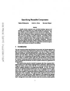
To effectively traverse such hierarchies a clear interpretation of each split-point is required. However, when natural language is used, a word’s semantics in general is context dependent and subject to human interpretation. If everybody generating or analyzing a description departs from an identical frame of reference, no problem occurs. But this is not the case if software development for reuse does not happen within the same context as software development with reuse [15, 1]. This may lead either to misclassifications or to an exploding number of descriptors. Domain specificity helps with these problems but is not a general solution. Human interpretation of natural language based descriptors is error-prone. Much research effort has been spent on finding alternatives to keyword based description techniques (cf. [11] for a survey on software libraries and retrieval techniques). Due to their rigid semantics, formal specifications suit very well for capturing the behavior of software ([6, 25, 10, 13]). When searching for a certain asset, the query is formulated as a (partial) specification. The retrieval process is then performed by conducting a formal proof that a component’s specification fulfills at least the needs expressed in the query. Unfortunately, formal methods in general are not widely accepted by developers. Thus, it is hard to push reuse concepts and to introduce new formalism at the same time. If developers are not comfortable with a technique or its application within the software development process, all the effort spent on building up a valuable repository vanishes. The formal nature of software requires some rigid description though. To overcome the (emotional) bottleneck described, we have to consider an alternative for fine grained search. Nevertheless such approaches have to be free from the need for human interpretation, while allowing software developers to retrieve components without extensive training in an intuitive manner. This paper deals with component retrieval for reuse. The context of the work reported here is shown in figure 1. We do assume that we depart from a large domain specific universe of components. With informal descriptions [3] and with generalized signature filtering [5] a coarse grain set of potential match components is identified. This set is further filtered according to semantic descriptions based on specific input-output tuples (data points) yielding a single (or very few) candidate component(s). In this paper we focus specifically on fine grained search. The basic idea is to exploit test cases as initial knowledge source for representing the functionality of components. The idea of considering test cases as partial specifications is also exploited in system analysis and system design [20, 2]. Augmented test cases (data points) are then classified by using a decision tree algorithm. The resulting hierarchical indexing structure supports interactive searching and browsing without the need for extensive user training.

informal description Universe of reusable components Coarse grain candidate set

domain specific components

data points

candidate set

signature

Figure 1. Query refinement for high precision

This paper is structured as follows: First we describe the requirements for data points to adequately describe the semantics of a repository’s components. Next we check to which extent these data points satisfy the criteria needed for applying decision tree algorithms. The approach is then demonstrated by two examples from different domains.

2. Data Points as Software Descriptors 2.1. Basic Principle We depart from the work of behavior sampling [19, 8], where retrieval of components is based on the inherent property of software which distinguishes software from other types of information: its executability. In behavior sampling, a query is formulated as a set of input-output examples, representing the main characteristics of the functionality searched for. The repository system then selects all components with respect to the interface signature induced by the examples. The next step is to execute these components on the input specified by the examples. If the output of the executed asset matches with the specified output of the examples, this asset is added to the candidate-set. The basic idea of behavior sampling is very promising, because the searcher is only concerned with the behavior of a component and must not bother with the interpretation of keywords or the structural aspects of the repository. Its main drawback, though, is that components need to be executed during the retrieval process. Thus, browsing the repository becomes inherently difficult. Furthermore, building and maintaining an execution engine for all components might outweigh the benefits of the library. We strive to overcome these drawbacks by shifting execution from the time of retrieval to the time of storing components [14]. Based on the claim that reusable components have to be of superior quality one can assume that they are carefully tested. These test cases represent a substantial cross section of a component’s functionality and could serve as a special form of description. Following the approach of behavior sampling we consider this data as execution history to be exploited instead of executing the component every time a query is entered.

Let us mention here one important thing. Behavior sampling tries to describe components according to their behavior based on input-output relations. Therefore, it is sufficient to have input-output pairs available, which are able to distinguish between various components. Testing on the other side is concerned with analyzing input-output tuples to state the quality of one component. This leads to the conclusion that indeed testing is not enough to determine the unique behavior of reusable components. But a portion of the test data of similar components (in the sense of signatures) can be sufficient to distinguish between components.

2.2. How to search Obviously, it is impossible for a searcher to have a presentiment of the queries covered by the test data. Nevertheless, the searcher has to be in a position to formulate adequate queries or to conduct an efficient dialog with the system. But how can this dialog be guided in a behavior driven search mechanism? We do so by taking the initiative and offering the searcher examples, changing the search process to a browsing one. In doing so, the searcher judges the importance of an example presented. If the offered behavior is covering the functionality searched for, the search is continued. If not, the searcher tracks back to the selection point of a previous decision and evaluates it once more. So the search is guided by browsing through the stored behavior and therefore the tuples presented should be highly discriminative and easily interpretable. To offer good examples to the searcher, the whole set of the test data must be analyzed and structured according to the available components. This task is accomplished by automatic classification performed by an supervised learning mechanism. The following section describes the conceptual organization of the repository. Since test cases generally are not well suited to serve this purpose the next two sections discuss some preconditions which must be fulfilled to allow automatic classification. These preconditions then affect the technical infrastructure of the repository as well as the test environment and the components themselves.

2.3. Repository Structure The index structure of the repository must reflect the special needs arising from a case based description. Following the ideas of [24] we cluster the repository into partitions with respect to the signatures of all reusable components. Thus, a partition p contains assets which conform with the signature p only. However, to allow a higher level of recall we use generalized signatures by extending the ideas of [17] and [24]. A generalized signature describes the coarse structure of a signature, respecting application semantics, but neglecting implementation details [15].

Starting point is an analysis of the data types of a signature, their qualification (the name of the parameter, the local position within the signature and the passing mode IN, OUT or INOUT) and their relation to other already known types. On the basis of type equality relations we analyze concrete signatures of procedural code and reduce them to function types [5]. These function types are flat representations of signatures in the sense that structures are disintegrated. Function types then are ordered in a lattice-like structure to allow for relational queries against the structure. Up to now, occurring ambiguities have been resolved by a human expert according to the special needs stemming from the repository structure. This is similar to the proposal of [4], where it is a developer’s or a librarian’s duty to annotate signatures with an abstract annotation for describing special properties. In our approach, every time a new generalized signature is added to the index, it must be judged to use an existing one or to build a new one. The following example demonstrates this process with a simple signature built on basic types. Example: If it is not important to distinguish between the C-data types long and double, these types are considered as substitutable. E.g. a C-function double fx1(long y) and a C-function long fx2(double z), might be in the same partition because both conform to the same generalized signature [number ! number].  On the basis of generalized signatures the repository is divided into partitions: for every signature p there exists an attached partition. An entry to a partition is then a component package containing one or more components (if they behave identically) and all the test data necessary to distinguish the behavior of one component from all other component packages in that partition.

2.4. Choosing Data Points Data points serve as descriptors for reusable software components. The main source for data points are test cases, which are available for free from the quality assurance process. But testing is primarily not performed to describe the behavior of software but to reveal faults and to raise the level of confidence in a component’s quality. To be valueable for component description, a test suite should be able to discriminate cj from the universe of all other possible functionalities in p . During the testing process, a vast amount of test data is generated. For the classification itself, only a narrow, but well chosen cross section of that data is sufficient. Hence, within the large set of given examples (test cases) useful ones are likely to be found, i. e. characteristic input-output tuples. Characteristic tuples strive for stimulating unique behavior such that on entering equal input for different components, they calculate different output [14].

PartitionΣ p

Components

C1

C2

C3

i1

O11

O12

O13

i2

.. .

O21

.. .

O22

.. .

O23

.. .

O24

im

Om1

Om2

Om3

Om4

Input

C4

O14

.. .

. . . . . .

. . . . . .

. . . . . .

. . O1n . O2n . .. . . . Omn Cn

Figure 2. A description of a library’s partition In figure 2 a sketch of the structure of a partition p is shown. Here n components c1::j::n are indexed, all of them executed with all given m inputs i1::k::m . The result ok;j = cj (ik ) of each test is entered into the corresponding place in the matrix. Hence, the pair (ik ; ok;j ) is an example of the behavior of cj . Column j contains the set of output values computed by cj . The matrix obtained serves as fine grained description of the sub-universe of components satisfying a particular signature.

2.5. Repository Maintenance Repositories are not built only once and don’t stay untouched forever. They are intended to be a long term investment and therefore content and structure must be adapted to reflect changing needs. During the life time of the repository new components are added repeatedly and likewise assets are removed. These operations erode the existing clustering and indexing structure. If a component is added, the available inputs of that partition must be analyzed concerning the ability to generate discriminating behavior. If no discriminating power for the added components is found on the basis of the available test data, new classification cases must be entered. Otherwise, as a result either ambiguous or incomplete descriptions and consequently classifications with a small degree of discrimination are produced. This

situation is sketched in Figure 3. Here, three added components do not completely fit into the data point space of the existing partition. As a consequence, new classification cases (indicated by the hatched area) have to be added to the data base. This leads to the following questions: (1) How can we retest the initial components on the new input and (2) how can we ensure that new components are tested with respect to the existing input in the repository. classified components

0110 100110 10 input

However, one has to acknowledge that data points resulting from quality assurance are defined with focus on a specific component. Discrimination against the universe of all possible functions in p is rather an illusionary vision. Here, we have to consider the component in the specific context of other assets in p and full discrimination must be guaranteed. To do so, additional data points for discrimination are needed. To obtain this automatically, we want to make sure that the components in the classification database have been executed with all inputs of that partition p . (Note: p contains assets with equal signatures). We refer to this property as initial completeness of the classification base. Initial completeness is also important for the classification algorithm we will describe later on.

initial classification space

(1) ?

10 (2)01 ?01 0000 1111 0000 1111 0000 1111 0000 1111 0000 1111 added components

added data points

Figure 3. Maintenance of partition

After adding new assets to a keyword based repository systems , a reindexing process updates the search paths. In our case this is not sufficient, since every component added not only enriches the description set with new tuples, but adds new descriptor tuples to already existing components! This effect may invalidate the existing indexing structure. As a consequence, simple reindexing after adding the new test cases is not sufficient. First, all missing tuples for already existing components must be generated, and second, test data of the fresh components must be completed. If these steps are performed, reindexing (reclassification) is easy and generates a correct indexing structure. The whole process of generating correct descriptions for all components within that particular partition must be repeated from time to time and then a reindexing has to be maintained. This impacts the testing process itself, such that from a tester’s perspective unnecessary tests for reuse purposes have to be conducted. To support the maintenance of the repository, test environments and test beds are an integral part of the reuse package. If the expected rate of component fluctuation is low, the knowledge for future reindexing can be obtained by storing a larger amount of data points as necessary initially.

2.6. Black Box Test Strategies Functional domain partition testing [16, 18] is the technique to generate test cases on the basis of the component’s purpose. According to the operational profile, tests are designed to split the input domain into different “use cases” (equivalence classes). The borders of such input partitions

are promising areas when looking for different behavioral variants included in the requirement, but not fully covered by the implementation. Functional domain testing is laborious, since it requires to have a complete specification at hand. Also the potential for automated tests is low. Random testing, on the other hand, does not bother about requirements driven input selection. Here, inputs are generated randomly according to a meaningful distribution. Only a large number of test cases provides a sufficient test coverage. Test case generation is obviously easy (if building the test oracle is as well). For classification purposes, domain partition testing and random testing on their own do not bring full benefit:

you want to determine the behavior of a sine function you are not interested in purely randomly generated input, but in specific values, such as 0; 4 ; 2 ; ; : : : to recognize the functionality immediately. For the reasons given above we combine both approaches: (1) The specific values obtained from domain partition testing are usually easy to interpret. Hence, they enable the reuser to use some of his/her application domain knowledge, thus helping to understand the classification. (2) Random testing lacks this feature but generates automatically sufficient data to enable automatic classification.

Domain partition testing: As domain partition testing is concerned with determining test tuples revealing component behavior, such characteristic pairs seem to be adequate for indexing and classification. Quite often, they have the nice property that human requesters can easily judge whether a particular input-output pair is adequate for the functionality s/he is looking for. But as classification is concerned with comparing features of a candidate with the features of other ones, we are also interested in inputs causing congruent output if executed on different components. We refer to such inputs as commonality points. Indeed, it is often the case that components with the same generalized signature belong to the same application domain and therefore significant common input data can be found for them. E.g. in the realm of mathematical functions, such a commonality point might be the input ’0’. But in general, the property of having equivalent signatures does not indicate the semantic proximity, making it difficult to find commonality points. Thus, there is an inherent difference between testing during the conventional software development process and using test values as data points for classification. The focus in classification is discrimination between concrete like components whereas the focus during testing is discrimination against the unspecific set of solutions not satisfying the specification at hand. Hence, data points resulting from domain partition testing (or whatever was considered as adequate testing strategy) has to be supplemented by further data points (see Section 2.4). We propose to generate those by means of random testing.

This section describes the process of building a classification structure on the basis of knowledge represented as data points. Here the technique of supervised learning is appropriate for solving the problem, because all classes (components) are known in advance. First, the necessary preconditions are stated and then we check whether they are fulfilled in the domain of data point analysis. Section 3.2 presents a short introduction to the algorithm we are using to classify the components.

Random Testing: Algorithms for automatic classification demand for a sufficient number of data points. This aim cannot be achieved by strictly following domain partitioning as criterion for data point selection. It can be reached easily by random testing though. A serious matter in relying on randomized input is the fact that the resulting classification structure (not the classification itself) is hard to understand. As an example, if

3. Analyzing data points

3.1. Prerequisites for Supervised Learning Due to the nature of repository classification we decided to adopt decision trees for analyzing classification data. Decision trees have the advantages that (1) their intuitive representation helps to understand the result, (2) the construction process demands the fact base, but no further parameters from the application domain are necessary, and (3) the error rate of a classification result is less or equal compared to all other classification mechanisms [7]. According to [22] the following properties must hold for a problem field to be suitable for decision tree algorithms. We briefly describe them and discuss if they are satisfied for repository classification based on data point descriptors. Property-value problem description: The problem must be described by a fixed number of attributes of discrete or continuous nature. Classification data analysis: How can we view test data in terms of attribute-value pairs? For every component we know the output value on every input available within the partition. Hence, we can look at the input values as properties of a component and the computed output as a value of this property. During initialization the number of input values is fixed because of the requirement of initial completeness (stated in section 2.4). Predefined Classes: All classes (categories) must be known in advance.

Classification data analysis: A class is an abstraction from individuals characterized by common properties. In our case, these properties are input-output values characterizing components. Therefore, a class in the field of machine learning is equivalent to the term reusable component. Discrete Classes: Classes must be disjunct. Classification data analysis: As we see from the previous paragraph, (functionally identical) components build a class, which leads to classes with one member only. The proposition is therefore automatically fulfilled. Sufficient Data: The algorithm depends heavily on a relevant amount of data to filter out coincidences. Classification data analysis: This is accomplished by combining domain partition testing with random testing, as described in section 2.6. Boolean decisions: All decisions are based on relational operations resting on attribute values. Deeper structures (as expressions in predicate logic) cannot be handled. Classification data analysis: Also this precondition is fulfilled, since every attribute must be instantiated with a value and no structural relations between the properties are given. As in our domain of test data analysis all preconditions are satisfied, we present in the next section the main characteristics of the C5-decision tree algorithm we are using to analyze the set of data points.

3.2. C5 – Decision trees The C5- (or See5) Algorithm of Quinlan [22] learns inductively hierarchical rules for determining classes from a set of attributed examples. It works recursively on the training set T of examples of classes T = fC1 ; C2 ; : : : ; Ck g. In every step three possibilities may occur: (1) The set of examples T is empty. C5 then generates a tree leaf, labeled with null. (2) All examples in T belong to one class Cj . C5 then generates a leaf, labeled with Cj (3) The examples in T belong to more than one class. C5 selects the most informative attribute am and generates a node labeled with that attribute am . For every value vmi of am (discrete type) or for a binary split (continuous type) C5 generates an edge labeled with vmi (discrete) or two edges  am , > am (continuous). The algorithm then determines the subset tj 2 T such that the attribute am contains value vmi (discrete case), ( am , > am in the continuous case). C5 builds a decision tree with tj nfam g and puts this structure to an edge labeled vmi , respectively ( am , > am ). C5 is able to classify classes described by continuous and discrete data. For continuous classes the most informative input is chosen to ensure a binary split of the class set

allowing a simple navigation in the classification hierarchy based on boolean decisions (see section 4.1 for details). Furthermore, C5 offers some nice features, especially the ability to set the minimum number of cases supporting the classification. In our context this is always ’1’, since for every component the quality of data points ensures, that only one attribute-value vector supports the classification.

4. Classification Examples In this section we present two examples. The first one classifies components in the domain of simple numerical calculations (continous output). The second one presents the classification of string predicates (discrete output).

4.1. A segment NUMBER

!

NUMBER

Here we analyze 32 Modula-3 functions with similar signatures from different packages. The 29 functions from the Math-package require one input parameter of type LONGREAL and return LONGREALs. The functions from the package Pts need a REAL as input and yield REAL as output. The SwapInt-function reverts the byte sequence of an arbitrary integer, INTEGER ! INTEGER. Hence, we choose NUMBER ! NUMBER as generalized signature for the partition. All functions are listed in figure 4. 1 2 3 4 5 6 7 8 9 10 11

Math.exp Math.expm1 Math.log Math.log10 Math.log1p Math.sqrt Math.cos Math.sin Math.tan Math.acos Math.asin

12 13 14 15 16 17 18 19 20 21 22

Math.atan Math.sinh Math.cosh Math.tanh Math.asinh Math.acosh Math.atanh Math.ceil Math.floor Math.rint Math.fabs

23 24 25 26 27 28 29 30 31 32

Math.erf Math.erfc Math.gamma Math.j0 Math.j1 Math.y0 Math.y1 Swap.SwapInt Pts.FromMM Pts.ToMM

Figure 4. The NUMBER!NUMBER MODULA-3 segment

The functions are tested with 128 test cases. This proved to be a sufficient number for a partition populated with 32 functions due to the C5’s information gain based selection of discriminating attributes. Normally, such a small number of tests tends to be very fragile with respect to the discrimination. But we designed our test bed to allow for repeated generation of test data, leading to the given high quality data points. Albeit, if continuous retesting cannot be established, the number of test cases must be significantly higher. Figure 5 shows a small fraction of the test data. Some symbolic values such as 1, ?1 or error which are also possible outputs are useful knowledge about component behavior and, therefore, they are included in the output space.

Input 60.45364 759.54846 214.51063 -107.50820 254.84983 -600.62990 -220.66893 -410.21593 21.82793 -881.66637

exp 23.13051 3.88E-56 0.00E+00 0.00E+00 0.00E+00 4.26E+213 1.80E+308 2.12E+54 1.80E+308 1.44E-23

gamma 0.82726 -493.23063 -5529.82350 -4608.86150 -4406.58105 2554.85263 4373.35105 477.48241 4346.32660 -157.53114

sin 0.00000005 -0.93741400 -0.84772226 0.96978008 0.66219540 0.97112202 0.98276884 -0.54213460 -0.44554438 -0.72567260




































. . .

. . .

. . .

. . .

.

.

.

Figure 5. An excerpt from the partition

759.5484572962105 -1: Math.sin : 759.5484572962105 81377.4: Math.expm1 : 117.79561660815057 -0.937414: :...-655.1335755461366 -Inf

o