Self-Motivated, Task-Independent Reinforcement Learning for Robots

Self-Motivated, Task-Independent Reinforcement Learning for Robots Lisa A. Meeden Computer Science Swarthmore College Swarthmore, PA 19081 [email protected]

James B. Marshall Computer Science Pomona College Claremont, CA 91711 [email protected]

Abstract This paper describes a method for designing robots to learn self-motivated behaviors rather than externally specified behaviors. Self-motivation is viewed as an emergent property arising from two competing pressures: the need to accurately predict the environment while simultaneously wanting to seek out novelty in the environment. The robot’s internal prediction error is used to generate a reinforcement signal that pushes the robot to focus on areas of high error or novelty. A set of experiments are performed on a simulated robot to demonstrate the feasibility of this approach. The simulated robot is based directly on an existing platform and uses pixelated blob vision as its primary sensor.

Introduction The quest for creating robot control systems that undergo an autonomous and extended developmental learning process was initiated by Weng and his colleagues (Weng et al. 2001). In their report, they differentiate the field of developmental robotics from traditional robotics by focusing on task-independent learning. Rather than building control systems to perform specific, predefined tasks, developmental robotics seeks to create open-ended learning systems that continually adapt to new problems. A number of robot control architectures have been created using this paradigm (Weng & Zhang 2002; Almassy, Edelman, & Sporns 1998), many of which involve some form of reinforcement learning. Reinforcement learning is an appealing approach because it provides a method for giving feedback to a developing system without having to specify how to succeed. Instead, the system is simply rewarded or punished, and must determine on its own how to behave so as to maximize its reward. However, there is no consensus yet about the most appropriate source for the reinforcement signal in a developmental robotics system. The reinforcement could come from an external teacher, from an internal mechanism such as emotion, or from a combination of external and internal sources. For example, the SAIL robot, an early prototype of a developmental learning system, depended on external reinforcement. SAIL could learn to navigate the corridors of a building by being manually pushed by a human teacher, or by having the teacher press the robot’s “good” button or “bad” button in response to its behavior (Weng et al. 2001). A

Douglas Blank Computer Science Bryn Mawr College Bryn Mawr, PA 19010 [email protected]

more recent version of SAIL employs a reinforcement signal that is the weighted sum of both external reinforcement and an internal measure of novelty (Huang & Weng 2002). The system compares the predicted next state to the actual next state, and if the prediction is incorrect, novelty is considered to be high. The intent of introducing novelty is to model habituation, as when human babies get bored by constant stimulation and are attracted to novel stimuli. In the SAIL system, the external reinforcement is weighted much more strongly than the internal novelty detection. Therefore the external teacher can easily override the internal drive to perceive new things. We believe that a key step in exploring developmental architectures is to focus on internal sources of reinforcement. The learning process should be driven by self-motivation, that is, by the system’s own internally-generated representations and goals, instead of relying on those provided by a teacher or designer outside the system according to some specific task to be learned. We are interested in developing a general learning architecture with self-motivation at its core, along with the other key processes of abstraction and anticipation (Blank et al. Forthcoming). We envision a control system in which abstraction, anticipation, and self-motivation are closely intertwined and develop together from the start within a single unified framework, using both internal and external sources of reinforcement. Such a system would build up abstractions of its experiences over time, guided by its internal motives, while learning to anticipate the effects of its sensorimotor interactions with the environment. An important advantage of self-motivated systems is that they can exhibit a degree of open-endedness not possible for systems that are designed to learn specific tasks. For example, the human capacity for learning is not only generalpurpose and task-independent, but typically continues over a lifetime, becoming progressively more complex and sophisticated in the types of abstractions and behaviors that can be acquired. The learning tasks themselves may change over time, as different circumstances and goals arise, but the impetus to adapt is ever present. How does this self-driven pressure to learn arise? In our view, it emerges from the interactions of other competing pressures within the system, in a manner reminiscent of a co-evolutionary arms race, in which two co-evolving species

continually push each other toward ever greater complexity. For example, such a system might attempt to predict future states as accurately as possible, while also attempting to seek out unanticipated, novel states. In effect, these two pressures compete directly against one another, since a system able to perfectly predict future states would never encounter any novelty, and a system that regarded everything it saw as new and unexpected would be incapable of predicting anything. However, if these pressures are balanced appropriately, the system might be able to “bootstrap” its way to increasingly sophisticated behaviors and organization. In other words, by seeking out situations with enough novelty to be interesting without being overwhelmingly unpredictable, the system might achieve a kind of temporary “homeostasis” balanced between surprise and predictability. Gradually, the system would gain the upper hand as it learned to anticipate unexpected things better, and its level of “boredom” would increase, in turn pushing it to explore its environment in search of richer, more interesting experiences. On the other hand, too much surprise would cause it to seek out more predictable regions of the environment. The result would be a type of punctuated learning in which the system remains at a given level long enough to master the tasks at hand, before moving on to the next level. Clearly, such a capability would depend on having a robust, generalpurpose learning system that could deal with the multitude of different learning tasks that would arise as the system’s experiences and behaviors increased in complexity.

Algorithm and Architecture In this section we propose a neural-network based reinforcement learning architecture to address these issues, in which discrepancies between the predicted outcomes and the actual outcomes of the robot’s actions in its environment serve as the fundamental source of self-motivation, thereby determining what the robot will learn to do. Although this represents an innate bias built into the architecture, it is not task-specific. The hope is that given the right developmental learning algorithm “hard wired” into the system (whether by evolution or engineering), the robot will be able to learn appropriate task-specific behaviors through its own experiences, guided by internally-generated feedback. Under control of the neural network, the robot generates motor actions to perform, along with predictions of the effects of these actions on its current situation. In our model, situations and predictions consist of simple two-dimensional visual scenes, but other types of sensory representations could be used. After performing an action and observing the results, the robot’s prediction is compared with the actual outcome, and a representation of the prediction error is created. This representation forms the basis of a reinforcement training signal for the network, using a version of Complementary Reinforcement Backpropagation (CRBP) (Ackley & Littman 1990). In CRBP, continuous-valued output activations from a network are transformed into binary values stochastically, typically by flipping a biased coin using the output activations as biases. Depending on the particular binary output

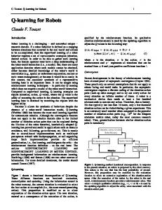
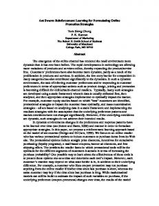
pattern generated, the network may receive reward or punishment as feedback. In the case of reward, the network’s weights are changed using backpropagation with the binary pattern itself as the training target. In the case of punishment, however, the complement of the pattern is used. The stochastic nature of CRBP allows the network to learn using only positive or negative feedback signals instead of a fullysupervised training regimen, which is ideal from the point of view of a robot exploring its environment in real time. In our version of CRBP, the amount of stochastic noise involved in transforming continuous output values into binary can be varied dynamically, under control of the robot itself. We introduce a computational temperature parameter τ , ranging from 0 to 100, that controls the amount of noise used in generating motor action vectors and their complements. At low temperature levels, activation values are translated to 0 or 1 nearly deterministically, while at high temperature the translation is nearly random, with 0 or 1 chosen essentially independently of the activation value. At intermediate temperatures, the translation function is a sigmoid curve of the general form 1/(1 + e−α(x−0.5) ), with the steepness of the sigmoid depending on τ . Thus temperature acts as a knob that determines the amount of influence the activation values exert on the translation process, ranging from no influence when τ = 100 to complete determinism when τ = 0. Given the inherently temporal nature of prediction, we chose to use a Simple Recurrent Network (SRN) architecture (Elman 1990), shown in Figure 1. There are separate banks of units for representing the robot’s motor actions (Min and Mout ), sensory state (S), sensory prediction (P), and temporal context (C), with each bank fully-connected to the hidden layer. The purpose of the network is twofold: to generate motor actions for controlling the robot, and to generate predictions that in turn guide the training of the network itself. Prediction and control are interleaved during the training process, with different banks of input and output units active at different times. Since the choice of motor action depends on the robot’s current sensory state and temporal context, banks Mout , S, and C are active when deciding what to do next, with Min and P disabled. Predicting the next state depends on which motor action is performed given the current state and context, so banks Min , S, C, and P are active during prediction, with Mout disabled. Some weights of the network (namely, those from the state and context banks to the hidden layer) participate in learning both the control and prediction tasks, reflecting their closely intertwined relationship, while others are specific to one task or the other. The training algorithm can be understood in terms of three general phases. In the first phase, internal feedback signals are generated from the robot’s prediction error. A representation of the prediction error is created based on the discrepancy between the robot’s actual observed state and its prediction made on the previous time step, and from this a reinforcement signal is computed. Temperature is also updated on the basis of the prediction error. Recall that the temperature ranges from 0 (deterministic) to 100 (random). Currently there are only two cases

Figure 1: The network architecture

when the temperature is not set to 0. The first is when there is no error centroid, which corresponds to perfect prediction. In this case, the temperature is set to 100 to induce exploration. The second is when the error centroid has remained stable between two successive steps, but is not centered. In this case, the temperature is set to 50. Learning occurs during the second phase. First, the network weights responsible for motor control are updated using CRBP, based on the reinforcement signal from phase one. This corresponds to behavioral learning, which is driven by discrepancies in the robot’s own internallygenerated anticipations, rather than by feedback coming directly from the environment or an external teacher. Next, the network weights responsible for prediction are updated, using ordinary backpropagation with the robot’s actual observed state as the feedback signal. This corresponds to anticipatory learning, which is driven by the robot’s direct experience in the environment. In the final control phase, the network generates the next action for the robot to take, as well as a prediction of the outcome of taking that action, and then executes the action. A more detailed description of the algorithm is given below, outlining the steps performed at time t. At the beginning of Step 1, the following information is known: Mt−1 is the motor action performed by the robot on the previous time step; St−1 is the robot’s previous sensory state; Ct−1 is its previous temporal context; Pt−1 is the prediction, generated at time t − 1, of the robot’s sensory state at time t; and Et−1 is a representation of the prediction error at time t − 1, based on the discrepancy between St−1 and Pt−2 . • Generation of internal feedback 1. Observe the current sensory state St . 2. Compare St to Pt−1 and create a representation of the prediction error Et . 3. Compare Et to Et−1 and compute a reinforcement signal r of +1, −1, or 0, and a temperature τ between 0 and 100. • Learning phase 4. If r is positive, set the motor target Mtarget to Mt−1 . If r is negative, set Mtarget to the complement of Mt−1 . If r is zero, skip to Step 7. 5. With banks Min and P disabled, perform one backpropagation pass with inputs St−1 and Ct−1 on the state

and context banks, and Mtarget on the motor output bank. In the case of positive reinforcement, this makes the network more likely to produce Mt−1 given the state and context St−1 and Ct−1 . For negative reinforcement, however, the opposite action will be more likely. 6. With bank Mout disabled, perform one backpropagation pass with inputs Mt−1 , St−1 , and Ct−1 , and target St on the prediction bank. This makes the network more likely to correctly predict state St when performing motor action Mt−1 in state St−1 with context Ct−1 . Set Ct to the hidden layer activation pattern resulting from this step. • Control phase 7. With banks Min and P disabled, compute the activation of the output bank Mout using St and Ct as inputs to the network. Stochastically transform the continuous-valued activations of Mout into a binary motor representation Mt , with the amount of noise determined by τ . This step generates the next motor action for the robot to perform, given its current state and context. 8. With bank Mout disabled, compute the prediction Pt using Mt , St , and Ct as inputs to the network. This step generates the robot’s prediction of the next state given the motor action to perform and its current state and context. 9. Perform action Mt . 10. Set t equal to t + 1 and go to Step 1. When training with CRBP, it is often helpful to use a higher learning rate for positive reinforcement than for negative (Ackley & Littman 1990). A positive reinforcement signal provides evidence that the motor action just performed was a good response to the current situation, so a relatively large weight change helps to increase the likelihood that the robot will take the same action the next time it finds itself in a similar situation. Negative reinforcement, however, suggests only that the motor action was not a good thing to do, and offers no guarantee that the opposite action would actually have been better. In this case, using a lower learning rate helps to steer the network away from producing the same response in the future, while remaining somewhat noncommittal about what response the network should actually produce. Thus the learning rate to use in Step 5 above can be set dynamically in Step 4 according to the value of r. In addition, a separate learning rate for prediction may be used in Step 6 if desired.

State Representation The above algorithm does not specify exactly how representations of the prediction error Et are created in Step 2, or how reinforcement signals are computed from them in Step 3. In fact, the algorithm is fairly general, and does not depend on the particular representation chosen for robot states or motor actions. Furthermore, there is no requirement that robot states must contain purely sensory information from the external environment. States could contain additional proprioceptor information, as well as explicit representations of

more abstract information generated internally by the robot, such as the prediction error itself. In our current model, a state St is represented as a 40 × 10 gray-scale image of intensity values normalized to the range 0–1, generated from a simulated blob vision camera. Prediction error Et is represented as a 40 × 10 map of the error values obtained in Step 2 by subtracting the corresponding image values of St and Pt−1 , and normalizing to 0–1.

Internal Reinforcement Signal To compute the reinforcement signal in Step 3, we first compute the “center of mass” coordinate for each twodimensional error map Et−1 and Et , called the error centroid of the map. This coordinate is simply the weighted average of the two-dimensional coordinates of all 40 × 10 error values, weighted by the size of the error. In our experiments, we have used a binary weighting function in which the weight of the error is 1 if the observed value is significantly greater than the predicted value at that point in the map, or 0 otherwise. Other mapping functions are of course possible, such as weighting a value by the magnitude of the error. To compute the reinforcement, the error centroids of Et−1 and Et are compared. If the centroid has moved closer to the center of the error map from time step t − 1 to t, the reinforcement is positive; if the centroid has moved away from the center, the reinforcement is negative; if there is no error centroid, the reinforcement is also negative. This last case is intended to force the robot to seek out novelty, since perfect prediction will lead to punishment. This method of computing the reinforcement signal represents a built-in bias of the system. This can be thought of as an innate tendency of the robot to want to “focus” on regions of unanticipated activity in the visual field by moving them to the center of view. It is important to note, however, that the reinforcement signal is not based directly on visual input from the environment; rather, it is based on the robot’s own expectations of what it will see as a result of responding to its current situation. The training of the network is driven by this internally-generated error information rather than by externally-generated visual information.

Motor Representation A binary representation for motor actions is necessary in order to allow CRBP to be used for the training of the network’s motor responses. In Step 7 above, the continuousvalued activations of the Mout units are transformed into a binary vector Mt . By injecting stochastic noise into this process, the network gains the ability to nondeterministically explore its weight space. This is especially important in the case of negative reinforcement, in which the optimal training target is unknown. In the experiments described below, we used a simulated robot with only one degree of freedom of movement. The position of the robot was fixed at the center of its environment, with only its angular orientation allowed to change. We chose an 8-bit representation for the motor actions, where the number of ones in a pattern specified the robot’s rotation speed and direction. The order of the bits was irrelevant. For example, all-zeros represented turning left quickly,

all-ones represented turning right quickly, and an equal number of ones and zeros caused the robot to stop. Many different patterns, therefore, were potentially available for the network to use in representing a particular motor action, which gave the robot more flexibility in learning to generate its motor responses. Accordingly, the Mout bank in Figure 1 contained eight units. However, when a motor action is presented to the network as input, it is first translated back into a continuous-valued scalar in the range 0–1, in order to make learning easier for the network. The Min bank thus consisted of only a single unit.

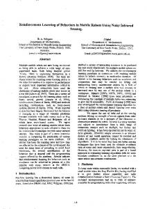
Experiments To test the architecture and the training algorithm, we created a simple environment in which the developing robot is fixed at the center of a circular arena and can rotate in order to observe its world. Also in the environment is a moving “decoy” robot controlled by an innate obstacle-avoidance behavior (see Figure 2). In some experiments, an additional stationary decoy robot was also present. The goal of the experiment is to induce the developing robot to attend to the moving decoy robot by tracking its motion. Clearly it should be possible to learn tracking by providing an external reinforcement signal that is based on whether the moving decoy robot is centered in the developing robot’s visual field. However, the more interesting issue is whether the developing robot can learn to track given only an internal reinforcement signal based on the error of its own predictions. In this case the external reinforcement signal is directly related to the task of tracking, while the internal reinforcement signal is more indirect. In the following experiments we compare the performance of a developing robot when using external and internal reinforcement signals. The performance measure is based on the average offset of the moving decoy robot from the center of the developing robot’s visual field. The experiments were conducted using the Stage mobile robot simulator (Gerkey, Vaughan, & Howard 2003), where the robot was a simulated ActivMedia Pioneer 2 (Act 2002) with a camera. The simulated camera had a 120-degree viewing angle centered on the front of the robot (indicated by the straight lines in Figure 2). Although the Stage simulator does not have simulated pixel-based camera output, we transformed Stage’s “blob” data into a 40 × 10 gray-scale image. When the decoy robot was in view, approximately 16 pixels (4% of the total image) were affected. The robot could turn to the left or right using one of 9 possible rotation speeds, as described earlier in the motor representation section. Using the robotics programming environment Pyro (Blank, Meeden, & Kumar 2003), we constructed the neural network shown in Figure 1, where the input layer had 1 motor-in unit, 400 state units, and 30 context units, the hidden layer had 30 units, and the output layer had 8 motor-out units and 400 prediction units. Using Pyro, the network was trained with the three-phase procedure from the algorithm section. The moving decoy robot continually roamed around the inside circumference of the circular wall. It started on the

1

Performance of Tracking Error Centroid

0.8

0.6

0.4

0.2

0 0

20

40

60

80 Trials

100

120

140

Figure 2: View of the training arena in the Stage simulator

north side of the circle facing west and traveled to the left, following the circular wall as it went. When it reached the south side of the arena, we repositioned it at the starting point, but this time facing east. The moving decoy robot then traveled along the wall to the right, until again it reached a point approximately due south of the starting point. The purpose of this two-legged journey was to ensure that leftward and rightward motion were represented equally during training. The entire trip of the moving decoy robot constituted one training trial for the developing robot. Furthermore, whenever the moving decoy robot was restarted at the north side of the arena, the activations of all of the network’s context units C were reinitialized to 0.5. This occurred at the beginning and the middle of each training trial. In the first experiment, an external reinforcement signal was based on the visual centroid of the camera image. The robot received positive reinforcement if the visual centroid moved toward the center of the visual field, and negative feedback if it moved away. If the decoy robot was not in view, no learning was performed. We ran this first experiment with computational temperature turned off (i.e., set to 0) in order to see how well the robot could learn in the absence of noise. All of the runs attained a high level of performance within 10 training trials. The network architecture and training procedure enabled the robot to learn to track the robot easily. Of course, our real interest was in seeing if the robot could learn this task indirectly, by using its non-task-specific prediction error in place of the actual visual input as a reinforcer. Therefore, we altered the training procedure by basing the reinforcement signal on the movement of the error centroid rather than the visual centroid (as described in the internal reinforcement section), but otherwise kept the experiment the same. Although the learning process was slower using the non-task-specific reinforcement signal, the robot was still able to learn to track the moving decoy robot. The next section examines in detail one successful run of this second experiment.

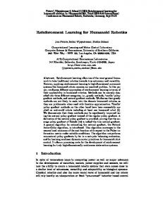
Figure 3: Performance of error centroid tracking over first 150 training trials

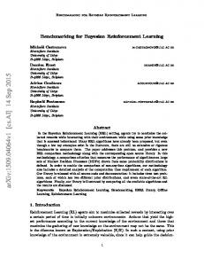
Analysis of a Training Run This run was representative of those that learned to track the moving decoy robot using only the internally generated reinforcement signal based on movement of the error centroid. As can be seen in Figure 3, initial performance was about 0.50, but quickly rose to above 0.80 within the first 40 trials. On trial 44 the performance of the network reached its peak, around 0.87. For comparison, we hand-coded a robot to perform the visual robot-tracking task, and it scored 0.92. A score of 1.0 is not possible because of the system’s inability to maintain the centroid in the exact center of view at all times. Recall that our system is designed to perform two conflicting tasks: to accurately predict the next state Pt+1 , but also to track the areas of its visual field where it cannot predict. Not surprisingly, the better the system is able to predict, the less it is able to track, resulting in a lower performance measure. From these competing goals, three recognizable phases emerge: an early phase (around trials 0 to 35) where the performance on tracking the moving decoy robot increases; a middle phase where the peak performance is attained (around trials 35 to 60); and a late phase in which tracking performance slowly declines (trials 60 and greater). Figure 4 shows representative camera images and prediction error data from the middle phase of this run. The left column shows a sequence of four camera images, with time running from top to bottom. The decoy robot can be seen as a square of gray pixels near the center of the visual field. The right column is the prediction error associated with each of the camera views. That is, the right column shows in black where the errors occurred on the prediction bank P at each of the steps in training. Notice that some of the prediction error regions are smaller than the associated regions from the camera image. This indicates that the system has begun to make some accurate predictions. The system re-

Figure 4: Sample camera images (left) and prediction error data (right) from the middle phase of learning

Figure 6: Sample camera images (left) and prediction error data (right) from the final phase of learning

0.9

1

0.85

0.8 TSS Prediction Accuracy

Performance of Tracking Error Centroid

0.8

0.6

0.4

0.75

0.7

0.65

0.6 0.2 0.55

0.5

0 0

200

400

600

800

1000 Trials

1200

1400

1600

1800

2000

Figure 5: Performance of error centroid tracking over all training trials

ceived negative feedback between the first and the second rows and again between the third and fourth rows (since the error centroids have moved slightly farther away from the center). Between the second and third rows, the network was rewarded, since the centroid moved toward the center of the field. Further examination of the tracking performance during the late phase shows that it continues to fall until the end of the run at trial 2000. Figure 5 shows the steady decline in performance and an increasing range of performance variability. To understand this behavior better, we can again examine camera images and prediction error. Figure 6 shows representative camera images on the left, and prediction errors on the right. Most noticeable is that in the first and fourth rows, there is no error in prediction. This resulted in reward between the first and second rows, and also between the second and third rows (as the centroid gets closer to the center). However, the system was again punished between the third and fourth rows as it “lost” the error centroid.

0

500

1000 Trials

1500

2000

Figure 7: TSS prediction accuracy over all training trials

Figure 7 shows that prediction accuracy is indeed climbing over the span of 2000 trials, albeit very slowly and also with increasing variability. Indeed, as prediction performance continues to increase in the late stage, the robot encounters fewer views containing any error at all, for which it is then punished. It is in this stage that the competing pressures discussed earlier are most apparent. If the experimental environment had been richer and more varied, after the developing robot had learned tracking, it would likely have been driven by its prediction error to focus on a new aspect of its world.

Discussion The defining characteristic of a developmental robotics architecture is task-independence. A developmental system must be open-ended and capable of finding interesting phenomena to focus on and learn about. The previous experiment demonstrated that a very general internal mechanism, such as an error centroid created from the robot’s own predictions, can serve as a successful reinforcement signal for

a developmental connectionist architecture. A limitation of the previous experiment is that the robot’s world was quite stark and uninteresting. Once the robot had learned to predict the decoy robot’s movements, there was nothing new to grab its attention. However, the idea of using error as a reinforcer is so general that this same mechanism should be equally capable of providing a useful reinforcement signal for other sensory modalities, as well as the fusion of multiple modalities. We plan to test our architecture in increasingly rich multi-modal environments. Another fruitful area of inspiration for creating generalpurpose internal reinforcement signals is the use of emotions (Gadanho & Hallam 1998). In Gadanho and Hallam’s work, a simulated Khepera robot is endowed with a set of homeostatic variables related to energy, pain, and restlessness. The environment contains a set of obstacles and a set of food sources. The robot’s energy decreases on every time step, and increases when it visits a food source. The robot’s pain increases when it bumps into obstacles and the robot’s restlessness increases when the robot is not moving. These homeostatic variables can serve to positively reinforce behavior that increases energy and negatively reinforce behavior that increases pain or restlessness. Currently, these reinforcement signals are only used to determine when to switch between a set of pre-programmed behaviors. Thus the robot is not developing any new behavior, but simply determining the best way to sequence its innate behaviors. In the current work, we have focused on a single homeostatic variable that strives to balance surprise and predictability. We would like to explore the level of complexity in behavior that is achievable using this sole self-motivating mechanism, but we envision that we will need to add other variables in future work.

Conclusions This paper defines a philosophy for designing systems with self-motivation. We believe that self-motivation is an emergent property generated by the competing pressures of developing accurate prediction and the desire to experience novelty. In addition we define a multi-step algorithm and simple recurrent network architecture that incorporates two learning systems based on these two pressures. One learning system attempts to make predictions of the next state while a second system uses a reinforcement signal based on error provided by the first to drive control toward novelty. Between these two competing forces, we believe, lies a rich area for learning. And in this framework lies a vast area for exploration in developmental robotics.

Acknowledgements We would like to thank Deepak Kumar, Paul Grobstein, Chris Prince, and the members of the Emergent Phenomena Research Group at Bryn Mawr for engaging discussions on this topic.

References Ackley, D. H., and Littman, M. L. 1990. Generalization and scaling in reinforcement learning. In Touretsky, D. S.,

ed., Advances in Neural Information Processing Systems 2. San Mateo, CA: Morgan Kaufmann. 550–557. ActivMedia Robotics, 19 Columbia Drive, Amherst, NH 03031. 2002. Pioneer Operations Manual, 11 edition. Almassy, N.; Edelman, G. M.; and Sporns, O. 1998. Behavioral constraints in the developmental of neuronal properties: A cortical model embedded in a real-world device. Cerebral Cortex 8:346. Blank, D.; Meeden, L.; Kumar, D.; and Marshall, J. Forthcoming. Bringing up robot: Fundamental mechanisms for creating a self-motivating, self-organizing architecture. Cybernetics and Systems. Blank, D.; Meeden, L.; and Kumar, D. 2003. Python robotics: An environment for exploring robotics beyond LEGOs. In ACM Special Interest Group: Computer Science Education Conference (SIGCSE). Elman, J. L. 1990. Finding structure in time. Cognitive Science 14(2):179–211. Gadanho, S. C., and Hallam, J. 1998. Exploring the role of emotions in autonomous robot learning. In Proceedings of the AAAI Fall Symposium on emotional intelligence: The tangled knot of cognition, 84–89. AAAI Press. Gerkey, B.; Vaughan, R.; and Howard, A. 2003. The Player/Stage project: Tools for multi-robot and distributed sensor systems. In Proceedings of the 11th International Conference on Advanced Robotics, 317–323. Huang, X., and Weng, J. 2002. Novelty and reinforcement learning in the value system of developmental robots. In Proceedings of the Second International Workshop on Epigenetic Robotics: Modeling Cognitive Development in Robotic Systems, volume 94, 47–55. Lund, Sweden: Lund University Cognitive Studies. Weng, J., and Zhang, Y. 2002. Developmental robotics - a new paradigm. In Proceedings of the Second International Workshop on Epigenetic Robotics: Modeling Cognitive Development in Robotic Systems, volume 94, 163–174. Lund, Sweden: Lund University Cognitive Studies. Weng, J.; McClelland, J.; Pentland, A.; Sporns, O.; I., I. S.; Sur, M.; and Thelen, E. 2001. Autonomous mental development by robots and animals. Science 291:599–600.