Issues in putting reinforcement learning onto robots - Semantic Scholar

Issues in putting reinforcement learning onto robots Jeremy Wyatt Department of Arti cial Intelligence, University of Edinburgh, 5 Forrest Hill, Edinburgh EH1 2QL, Scotland, U.K. March 25, 1995

Abstract

nd the best way to achieve a task as part of the process of designing a robot controller1. On-line learning is similar in many respects to our common-sense notion of `learning'. An agent, presumably with a large amount of knowledge about its task and environment, encounters a new situation. It must quickly grasp the correct course of action, and do so without intervention by the operator. In such circumstances there is little room for error, and hence a trade-o exists between exploring and exploiting the environment. In o-line learning the criteria for success are much simpler. The agent merely needs to maximise its performance on a task by the end of the learning period. We lose the need to exploit the environment because the agent's performance during the learning period doesn't matter. In addition the learning process need not be entirely autonomous. The designer may intervene in a number of ways. These could feasibly include driving the robot through some example solutions [5, 11]; decomposing the task into simpler tasks and then recomposing the solutions to these [14, 15]; or providing intermediate indicators of performance, i.e. telling the robot when it's doing well even if it hasn't achieved the goal yet [16]. This paper is concerned with problems in o-line learning. In particular it looks at o-line learning using Reinforcement Learning (RL) methods. The basics of RL will now be outlined before we discuss some of the dicul-

There has recently been a good deal of interest in robot learning. Reinforcement Learning (RL) is a trial and error approach to learning that has recently become popular with roboticists. This is despite the fact that RL methods are very slow, and scale badly with the size of the state and action spaces, thus making them dicult to put onto real robots. This paper describes some work I have been doing on trying to understand why RL methods are so slow and on how they might be speeded up. A reinforcement learning algorithm loosely based on the theory of hypothesis testing is presented as are some preliminary results from employing this algorithm on a set of bandit problems.

1 Introduction There are many ways in which we can think of categorising robot learning methods. One useful distinction is that between when the performance of the robot during the learning period matters and when it does not matter. In this paper the former will be refered to as on-line learning and the latter as o-line learning. An example of the rst is when a robot must cope with unforeseen situations while operating autonomously in pursuit of a goal; an example of the second is when we use learning to try to

1

1

See [2] for a similar distinction.

3 Problems putting RL onto robots

ties encountered when employing it in robots. A reinforcement learning algorithm will then be presented which is loosely based on the theory of hypothesis testing. Recently a lot of work has been done trying to put RL algorithms onto real robots and there have been a number of successful implementations to date [7, 9, 14, 15, 16, 19]. There however, a number of diculties associReinforcement learning is a trial and error ap- are, ated with RL methods per se and these are proach to learning in which an agent operat- especially to the problem of using ing in an environment learns how to achieve a them with pertinent real robots. short RL makes astask in that environment. The agent learns by sumptions which do notIn apply to real world adjusting its policy2 on the basis of positive tasks [16]. (or negative) feedback | termed reinforcement. This feedback takes the form of a scalar First RL assumes that the environment as value generated by the agent each time step, perceived by the agent is a Markov Decision high and low values corresponding to rewards Process (MDP). Informally this means that and punishments respectively. The mapping the agent only need know the current state in order to predict its future from environment states and agent actions to of the process 6 . If the agent does not have subehaviour reinforcement values is termed the reinforceto predict the future process ment function. The agent converges to the cient information 7 then what Whitehead terms perbehaviour behaviour maximising reinforcement (the optimal policy). In theory an appropriate re- ceptual aliasing [26] occurs. This is when an inforcement function3 exists for all tasks, al- agent cannot distinguish between two states though nding such a function is typically which are signi cantly dierent with respect to their behaviour under the same policy. New hard [1]. algorithms have been designed to cope with It is worth noting that unlike in supervised this phenomena 26] but are not guaranlearning procedures the error signal does not teed to converge [13, to the optimal policy under indicate which behaviour is correct, merely such conditions. how good or bad the current behaviour is relative to others. This means that in order to The second major problem is that of slow nd the best action in each state the agent convergence. Even in a perfectly determinmust try it at least once and hence in order istic Markovian environment RL takes time to guarantee converging to the optimal policy exponential in the size of the state space to the agent must try all actions in all states at converge to the optimal policy. In stochasleast once4 . In addition the feedback received tic environments with large state spaces (e.g. is usually delayed5 , and hence most work on a typical robot task) this means that times RL has been on solving the problem of as- to convergence are prohibitively long. There signing credit (or blame) to individual actions are necessarily two types of solution: either within a sequence leading to the receipt of make your temporal credit assignment mechreinforcement. This is known as the tempo- anism faster or make your temporal credit asral credit assignment problem (TCA). It is to signment problem simpler. The rst approach be distinguished from the better known struc- has manifested itself in two ways: work on tural credit assignment problem (SCA), which more ecient trace mechanisms [4, 20, 21, 24], is concerned with assigning credit to features and work on the use of generalisation methods of a state in order to generalise across states. [3, 17]. The second approach includes methods such as task decomposition [6, 10, 12, 15, 22, 8]

2 Reinforcement Learning

The mapping from environment states to agent actions. 3 i.e. one in which the policy maximising reinforcement corresponds to the behaviour which the designer considers optimal. 4 An in nite number of times if the environment is stochastic. 5 This is not necessarily the case e.g. the two-armed bandit task used here. 2

6 In principle any process can be represented as an MDP because an abitrary amount of information about the history of the process can be included in the description of the current state, e.g. we need to know the velocity and acceleration of a ball in order to be able to calculate its trajectory. 7 In the case of RL this means it does not have sucient information to predict average return accurately.

2

1 2 3 4 5 6 7 8 9 10

t=0 ni = xi = 0, 8i a(t) = aj such that  (aj )   (ai ); 8i update nj = nj + 1 if r(t) = 1 then xj = xj + 1 pj = xj nj pmax = max(pi ), pmin = min(pi ), 8i if Pr(Pmax ? Pmin  pmax ? pmin )   then drop amin t= t+1

goto step 3

Where  (a) is the width of the 100(1 ? ) con dence interval for action a; a(t) is the action at time t; and ni ; xi are the number of trials and successes for action ai . pi is the proportion of successes for action ai . Pi = Xi =ni, where Xi  bin(Xi ; ni; i).

Figure 1: Algorithm 1 | Based on hypothesis testing. 1 2 3 4 5 6

t=0

choose a(t). Pr(a(t) = a) = (a; t), 8a p(t + 1) = p(t) + (r(t  + 1) ? p(t)) (r(t + 1) ? p(t)) if a=a(t) (a; t + 1) = (a; t) + ? (a; t)  (r(t + 1) ? p(t))=(1 ? (a(t); t)) otherwise t= t+1 goto step 2

Where  is the agent's policy; r(t) and p(t) are the actual and predicted reinforcement values; and , are the learning rates for the policy and the value function respectively.

Figure 2: Algorithm2 | A variant of Sutton's reinforcement-comparison algorithm and the construction of better reinforcement functions [16]8. But even if we can solve all these diculties in one robot simultaneously (solutions to one problem tend to prevent solutions to other problems 9) we still have `lesser' implementational diculties such as the fact that RL algorithms are discrete when processes in the world are continuous. While RL is a very general, and hence weak AI method, robots present problems that require strong, and therefore speci c solutions. A tabula rasa approach to RL will not work in robots. Attempts to seed the robot behaviour with designer knowledge [5, 15, 16] need, if possible, to be systematised. The situation is

analogous to that faced by the expert systems community in the early 1980s. How do we transfer our expert's knowledge into our expert system? In this case how do we transfer our expert knowledge about how to operate in uncertain physical environments into our robots? One way round part of this robot knowledge acquisition problem is to teach a robot by driving it through a task along a nearoptimal solution several times [11]. But unless this is merely to become a form of supervised learning a principled means of integrating the taught (supervised) and exploratory (unsupervised) approaches is required. One method is to give an agent knowledge about how much it knows about dierent portions of the state space [18, 25]. In an oline learning methodology the agent must then explore the environment so as to maximise its knowledge about the task domain rather than in order to maximise short-term rein-

8 Even if a reinforcement function is appropriate in the sense outlined above it may still fail to give the agent sucient feedback to ensure speedy learning, and so may not be a good reinforcement function. 9 e.g. if we use a generalisation method then we risk over-generalising and thus exacerbating the perceptual aliasing problem.

3

forcement. In other words we cannot use pure exploitation policies or the agent may get trapped in the taught (and possibly suboptimal)behaviour. Being greedy with respect to knowledge can be better than being greedy with respect to rewards.

1

a = 0.0625 a = 0.125 a = 0.0312

0.9 a = 0.25 a = 0.0156

Performance

0.8

4 Reinforcement Learning using hypothesis tests

0.7

a = 0.5

0.6

a = 0.0039

0.5

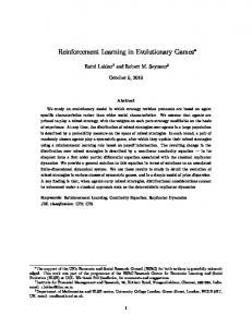
As mentioned previously, work on speeding up RL algorithms has concentrated on speeding up temporal credit assignment i.e. the rate at which the agent constructs estimates of the mean return for each state. We can however also alter the rate at which the policy is adjusted. The problem of setting learning rates for policies can be most easily and thoroughly studied in an envionment without the need for a secondary-reinforcement mechanism. The environment chosen here is a bandit-task of a kind already widely studied in the literature [9, 23]. Reinforcement is immediate and boolean. A summary of the tasks used is given in Figure 4. The performance of an RL algorithm such as the AHC algorithm [23] depends on being able to pick a good value for the learning rate for the policy, , and for the value function, 10 . Figure 3 shows that the performance varies as an inverted U-shaped function of . The optimal value of  roughly increases with the size of the dierence between the mean reinforcements for each action and decreases with its variance. Thus the optimal value of  can vary considerably across tasks. As the degree of uncertainty in an environment is usually unknown this makes RL algorithms hard to optimise. One way to overcome this would be to set the learning rate automatically11. Another approach is to remove the learning rate parameter altogether. This is the approach taken here in Algorithm 1 (see Figure 1). The algorithm works in the following manner. The agent is initially equally uncertain about all actions, so the probability distribu-

0.4 0

100

200

300

400

500 600 Timestep

700

800

900

1000

Figure 3: Performance of a variant of Sut-

ton's reinforcement-comparison algorithm (see Figure 2) on a 2-armed bandit task. The curves of the averge performance for dierent values of  are shown ( = ). Performance is scaled between the worst policy and the best policy: 1 is optimal, 0.5 is random. 0 = 0:55, 1 = 0:45. The gures were calculated from 100 trials of 1000 time steps each. tion across actions is uniform when t = 0. Each time step the action is chosen about which the agent knows least (step 3). This is the action with the widest binomial con dence interval on p, the proportion of successes. The statistics n, x and p are updated (steps 4 and 5). Then the best and worst looking actions are found (step 7). The agent hypothesizes that actions are equally good, and calculates the likelihood of this result on the basis of the observed results. If the observed dierence pmax ? pmin is unlikely on the 'null' hypothesis that the true rates of success for each action are the same (i.e. max = min) then this is rejected at the 100% level of signi cance and the alternative hypothesis that the best looking action is indeed better is accepted (step 8). In this case the action amin is dropped from the list of actions considered for execution. The calculations are made on the binomial distribution. Actions are not dropped in order that the environment be exploited more eectively during the learning period, but so that the environment may be explored more eciently. The algorithm has converged when all actions but one have been dropped. The nal result is an ordering on the set of all actions. The performance of this algorithm was

10 Work has already been done on setting automatically [24], but no such work has been done on setting . 11 e.g. by adjusting  according to the variance in the average return for each state (RC and AHC algorithms) or for each state-action pair (Q-learning).

4

Task Pr(r = 1) a0

0.9 0.55 0.9 0.2

a1

0.1 0.45 0.8 0.1

1

0.98

Performance

1 2 3 4

Figure 4: Table of the 2-arm bandit tasks

used. R = 0; 1. Each pull on an arm is a Bernoulli trial. For convenience a0 is always optimal.

0.96

0.94

0.92

rc(0.5,0.1) algorithm 1 (0.05)

tested against a variant of Sutton's reinforcement algorithm on the four twoarm bandit tasks described in Figure 4. The reinforcement-comparison (RC) algorithm used was optimised across , being set to the same value except in the case of Task 1 where = :1 was found to be optimal. For both algorithms and all tasks 200 simulation runs were made, each of 2000 timesteps. For each step in each run the scaled performance of the exploitation policy the agent currently considers best was recorded. Note that for the agent using Algorithm 1 this is not the actual reinforcement generated during the learning run, but an estimate of how much the agent has learned about the task in the form of a recommended exploitation policy. The recommended exploitation policy for Algorithm 1 is a uniform distribution across the remaining eligible actions. The exploration policy is the one followed during the course of the learning period. The scaled performance is calculated using equation 1. p=

E [R]c ? E [R]w E [R]o ? E [R]w

0.9 0

50

100

150

200

250 300 Timestep

350

400

450

500

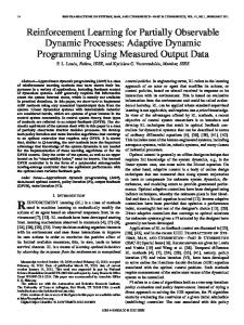
Figure 5: Curves of the mean performance

of Algorithm 1 (see Figure 1) and a variant of Sutton's RC algorithm (see Figure 2) on Task 1. Performance is scaled between the worst policy and the best policy: 1 is optimal, 0.5 is random. 0 = 0:9, 1 = 0:1. Both algorithms were run for 200 trials, each of 2000 time steps. The parameter  of Algorithm 1 was set to 0.05. For the RC algorithm  = 0:5 and = 0:1.

1 0.95 0.9

Performance

0.85 0.8 0.75 0.7 0.65

(1)

0.6

rc(0.0312)

0.55

algorithm 1 (0.05)

where R is the random variable denoting return, and c, o and w denote the current, optimal and worst policies respectively. 6: Curves of the mean performance Figures 5-8 show the mean performance for Figure of Algorithm 1 (see Figure 1) and a variant each algorithm over 2000 timesteps. of Sutton's RC algorithm (see Figure 2) on Task 2. Performance is scaled between the worst policy and the best policy: 1 is optimal, 0.5 is random. 0 = 0:55, 1 = 0:45. Both It can be seen from Figures 5-8 that on Tasks algorithms were run for 200 trials, each of 2000 2 and 3, Algorithm 1 converges signi cantly time steps. The parameter  of Algorithm 1 faster than the reinforcement-comparison al- was set to 0.05. For the RC algorithm  = gorithm. On Tasks 1 and 4 it converges at = 0:0312. about the same rate. On Tasks 2 and 4 how0.5 0

5 Discussion

5

200

400

600

800

1000 1200 Timestep

1400

1600

1800

2000

1

0.95

0.95

0.9

0.9

0.85

0.85

0.8

0.8

Performance

Performance

1

0.75 0.7 0.65

0.7 0.65

0.6

0.6

rc(0.0312)

0.55 0.5 0

0.75

algorithm 1 (0.05)

200

400

600

800

1000 1200 Timestep

1400

1600

1800

rc(0.125) algorithm 1 (0.05)

0.55 0.5 0

2000

200

400

600

800

1000 1200 Timestep

1400

1600

1800

2000

Figure 7: Curves of the mean performance Figure 8: Curves of the mean performance

of Algorithm 1 (see Figure 1) and a variant of Sutton's RC algorithm (see Figure 2) on Task 3. Performance is scaled between the worst policy and the best policy: 1 is optimal, 0.5 is random. 0 = 0:9, 1 = 0:8. Both algorithms were run for 200 trials, each of 2000 time steps. The parameter  of Algorithm 1 was set to 0.05. For the RC algorithm  = = 0:0312.

of Algorithm 1 (see Figure 1) and a variant of Sutton's RC algorithm (see Figure 2) on Task 4. Performance is scaled between the worst policy and the best policy: 1 is optimal, 0.5 is random. 0 = 0:2, 1 = 0:1. Each algorithm was run for 200 trials, each of 2000 time steps. The parameter  of Algorithm 1 was set to 0.05. For the RC algorithm  = = 0:125.

ever it converges to a signi cantly poorer policy on average than the RC algorithm. Why is this? There is a probability that at each timestep the observed results will cause the null hypothesis (0 = 1) to be rejected in favour of the alternative hypothesis 1 > 0. The algorithm then converges to a sub-optimal policy. The probability of such a result gets larger as the dierence between 0 and 1 decreases, and as the variance in p0 and p1 increases. This is why the algorithm converged to such a poor policy on Task 2. There are two possible solutions to this problem: either the signi cance level of the test can be altered dynamically during the learning period in order to keep the probability of an error low; or more simply, actions can become eligible again if the dierence between them and the best action falls outside the critical region once more. This process of unsticking the algorithm would be strengthened by retaining a small probability each timestep of executing one of the actions that the agent has rejected. These strategies are currently being implemented and tested. It is signi cant that Algorithm 1 performs reasonably on all tasks with the same value for , whereas the RC algorithm must be op-

timised with respect to both  and . This paper has argued that RL methods making better use of the information available to them and when combined in a principled manner with teaching methods do have the potential to be fast enough to scale to learning more complex robot tasks. A new algorithm has been presented based on the theory of hypothesis testing, and some initial results presented that show some promise. While it is clearly not the case that the algorithm presented here is ideal, the results indicate that algorithms of a similar kind may have potential. There are a number of extensions that need to be carried out to this work. First a means for reducing the error rate for Algorithm 1 must be found. Secondly more complex bandit trials should be carried out to con rm that the advantage scales to higher numbers of actions. Thirdly, although this algorithm is designed to work only on bandit problems with boolean reinforcement, (i.e. there must be no state, and no unbalanced or delayed reinforcement) the general method should be extendable to problems with unbalanced reinforcement12 and hence to any 12

6

In the manner of Kaelbling's interval-estimation

[8] Jonas Karlsson JoshTenenberg and Steven Whitehead. Learning via task decomposition. In From Animals to

method where a value function on the state space is available.

Acknowledgements

Animats 2: Proceedings of the 2nd International Conference on the Simulation of Adaptive Behaviour, pages 337{343. MIT

Thanks go to Gillian Hayes, John Hallam and Martin Westhead for many valuable discussions on the topics herein, and for comments and advice on the production of the paper. Jeremy Wyatt is in receipt of SERC Research Studentship No.92314758.

Press, 1992. [9] Leslie Pack Kaelbling. Learning in Embedded Systems. PhD thesis, Dept of Computer Science, Stanford, 1990. [10] Leslie Pack Kaelbling. Hierarchical learning in stochastic domains: preliminary results. In Machine Learning: Proceedings of the 10th International Conference, pages 167{173, 1991. [11] Long-Ji Lin. Programming robots using reinforcement learning and teaching. In

References

[1] A. G. Barto. Connectionist learning for control. In W. T. Miller R. S. Sutton and P. J. Werbos, editors, Neural Networks For Control, pages 5{58. MIT Press, 1990. Proceedings of the ninth national confer[2] Rodney A. Brooks and Maja J. Mataric. ence on arti cial intelligence, pages 781{ Real robots, real learning problems, chap786. AAAI Press/MIT Press, 1991. ter 8, pages 193{214. Kluwer Academic Publishers, 1993. [12] Long-Ji Lin. Hierachical learning of robot [3] David Chapman and Leslie Pack Kaelskills by reinforcement. In Proceedings bling. Input generalisation in delayed reof the IEEE International Conference on inforcement learning: an algorithm and Neural Networks 1993, pages 181{186, performance comparison. In Proceedings 1993. of International Joint Conference on Ar[13] Long-Ji Lin and Tom M. Mitchell. Reinti cial Intelligence, 1991. forcement learning with hidden states. In [4] Pawel Cichosz. Truncating temporal difProceedings of the Second International ferences: on the ecient implementation Conference on the Simulation of Adaptive of td() learning. Journal of Arti cial Behaviour. MIT Press, 1992. Intelligence Research, 2:287{318, January [14] P. Maes and R.A. Brooks. Learning to 1995. coordinate behaviours. In Proceedings of [5] Marco Colombetti and Marco Dorigo. the 8th National Conference on AI, 1990. Training agents to perform sequential behaviour. Submitted to the Journal of Evo- [15] S. Mahadevan and J.H. Connell. Automatic programming of behaviour-based lutionary Computation, September 1993. robots using reinforcement learning. Re[6] P. Dayan and G. Hinton. Feudal reinsearch Report RC 16359 (72625), IBM forcement learning. In S.J. Moody J.E., Research Division, July 1990. Hanson and R.P. Lippmann, editors, Advances in Neural Information Processing [16] M. Mataric. Reward functions for acSystems 5, pages {. Morgan Kaufmann, celerated learning. In W.W. Cohen and 1993. H. Hirsh, editors, Machine Learning: Proceedings of the Eleventh International [7] Marco Dorigo and Marco Colombetti. Conference, pages 181{9. Morgan KaufRobot shaping: Developing situated mann, February 1994. agents through learning. Technical Report TR-92-040 (revised), International [17] Matthew A.F. McDonald Computer Science Institute, April 1993. and Philip Hingston. Approximate discounted dynamic-programming is unrelialgorithm [9], so that the con dence intervals and tests are conducted based on the mean reinforcement. able. Technical Report 94/6, University 7

of Western Australia, Dept of Computer Science, October 1994. [18] Andrew W. Moore. Knowledge of knowledge and intelligent experimentation for learning control. In Proceedings of the

Report TR-331 (revised), University of Rochester, Department of Computer Science, June 1990.

International Joint Conference on Neural Networks, volume 2, pages 683{8, July

1991. [19] Ulrich Nehmzow. Experiments in Competence Acquisition for Autonomous Mobile Robots. Ph.d. thesis, Department of Arti-

cial Intelligence, Edinburgh University, 1992. [20] Mark Pendrith. On reinforcement learning of control actions in noisy and nonmarkovian domains. Tech report UNSWCSE-TR-9410, University of New South Wales, School of Computer Science and Engineering, August 1994. [21] Jing Peng and Ronald J. Williams. Incremental multi-step q-learning. In W.W.Cohen and H.Hirsh, editors, Ma-

chine Learning: Proceedings of the 11th International Conference, pages 226{232,

1994. [22] Satinder P Singh. The ecient learning of multiple task sequences. In S. Hanson J. Moody and R. Lippman, editors, Ad-

vances in Neural Information Processing Systems 4, pages 251{258. Morgan Kauf-

mann, 1992. [23] R.S. Sutton.

Temporal Credit Assignmenment in Reinforcement Learning.

PhD thesis, University of Massachusetts, School of Computer and Information Sciences, 1984. [24] R.S. Sutton and S.P. Singh. On step-size and bias in temporal dierence learning. In Proceedings of the Eighth Yale Workshop on Adaptive and Learning Systems, pages 91{96, 1994. [25] Sebastian B. Thrun. Ecient exploration in reinforcement learning. Technical Report CMU-CS-92-102, Carnegie Mellon University, School of Computer Science, January 1992. [26] Steven D. Whitehead and Dana Ballard. Learning to perceive and act. Technical 8