May 24, 2016 - 121 pencil box. 2.89. 3.52. 2.38. 2.62. 2.67. 1.95. 122 pencil sharpener. 1.49. 1.74. 1.20. 1.49. 1.34. 1.33. 123 perfume. 11.55. 5.99. 9.16. 8.62.
arXiv:1605.07651v1 [cs.CV] 24 May 2016
Self Paced Deep Learning for Weakly Supervised Object Detection
Enver Sangineto∗1 Moin Nabi∗1 Dubravko Culibrk2 Nicu Sebe1 1 2 DISI, University of Trento, Italy FTS, University of Novi Sad, Serbia {enver.sangineto,moin.nabi,niculae.sebe}@unitn.it,{dculibrk}@uns.ac.rs
Abstract In a weakly-supervised scenario, object detectors need to be trained using imagelevel annotation only. Since bounding-box-level ground truth is not available, most of the solutions proposed so far are based on an iterative approach in which the classifier, obtained in the previous iteration, is used to predict the objects’ positions which are used for training in the current iteration. However, the errors in these predictions can make the process drift. In this paper we propose a self-paced learning protocol to alleviate this problem. The main idea is to iteratively select a subset of samples that are most likely correct, which are used for training. While similar strategies have been recently adopted for SVMs and other classifiers, as far as we know, we are the first showing that a self-paced approach can be used with deep-net-based classifiers. We show results on Pascal VOC and ImageNet, outperforming the previous state of the art on both datasets and specifically obtaining more than 100% relative improvement on ImageNet.
1
Introduction
A well known problem in object detection is the fact that collecting ground truth data (i.e., objectlevel annotations) for training is usually much more time consuming and expensive than collecting image-level labels for object classification. This problem is exacerbated in the context of the current deep nets, typically composed of tens of millions of weights, which need to be trained either from scratch [14] or “fine-tuned” [9] using large amounts of data. Weakly-supervised techniques for object detection can alleviate the problem by leveraging existing datasets which provide image-level annotations only. In a Multiple Instance Learning (MIL) formalization of the weakly-supervised object detection, an image I, associated with a label of a given class c, is described as a “bag” of Bounding Boxes (BBs), where at least one BB is a positive sample for c and the others are samples of the other classes (e.g., the background class). The main problem is how can the classifier automatically guess what the positives in I are. A typical MIL-based solution alternates between 2 phases: (1) optimizing the classifier’s parameters, assuming that the positive BBs in each image are known, and (2) using the current classifier to predict the most likely positives in each image [6, 20]. However, if the initial classifier is not strong enough, this process can easily drift. For instance, predicted false positives (e.g., BBs on the background) can make the classifier learn something different than the target class. Kumar et al. [15] propose to use a self-paced learning strategy in a MIL framework. The main idea is that a subset of “easy” samples can be automatically selected by the classifier in each iteration. Training is then performed using only this subset, which is progressively increased in the subsequent iterations when the classifier becomes more mature. Self-paced learning, applied in many other ∗
Authors contributed equally.
T1 T2
T3 T4
t=1
t=2
t=3
t=4 …
Figure 1: A schematic illustration of how the training dataset Tt of our deep net evolves depending on t and on the progressively increasing recognition skills of the trained net.
studies [13, 16, 17, 18, 22], is related to curriculum learning [2] and is biologically inspired by the common human process of gradual learning, starting with the simplest concepts. In this paper we adopt a self-paced learning approach to handle the uncertainty related to the BB-class association in a weakly supervised scenario, thus “easy” is interpreted as “likely correct”. We propose a new training protocol for deep nets in which the self-paced strategy is implemented by modifying the mini-batch-based selection of the training samples. As far as we know, this is the first self-paced learning solution directly embedded in a modern deep-net training protocol. More specifically, the solution we propose in this paper is based on a recently proposed deep net architecture for (fully supervised) object detection: Fast-RCNN [8]. Fast-RCNN naturally embeds the idea of an image as a bag of BBs (see Sec. 3). Moreover, in the Fast-RCNN approach, each mini-batch of the Stochastic Gradient Descent (SGD) procedure is sampled hierarchically, by first (randomly) sampling images and then sampling BBs within those images according to BB-level ground truth information. We exploit this “image-centric” sampling but we replace the random image selection with a self-paced strategy in which the images with the highest-confidence boxes for each class are selected the first. In more detail, given an image I with an image-level label y, we use the net trained in the previous iterations to associate a class-specific score siy with each BB bi . The highest score box zI is selected in I. Note that, due to the spatial regression layer in Fast-RCNN, zI is usually a new box, i.e., the bag of BBs associated with I dynamically changes at every self-paced iteration. Once zI is chosen for each I in the training set, we select a subset of images according to the score associated with the corresponding zI and a mini-batch of positive and background BBs is extracted using zI . Moreover, since we train a multi-class classifier (a common approach in deep nets which exploit inter-category representation sharing [14]), we exploit the competition among classifiers of different categories (i.e., among different output neurons of the same net) and an image is chosen only when its label is consistent with the strongest classifier on that image. In summary, our contributions are the following. • We propose a computationally efficient self-paced learning approach for training a deep net for weakly supervised object detection. During the training of the net, the same net, at different evolution stages, is used to predict the class-specific positive BBs and to select the most likely subset of correct samples to use for the subsequent training stages. • We propose to use class-specific confidence and inter-classifier competition to decrease the probability of selecting incorrect samples. • We test our approach on Pascal VOC 07 and ILSVRC13, obtaining slightly better results in the former dataset and largely outperforming the state of the art in the latter (+100% relative improvement). The code will be published with the article. 2
2
Related work
Many recent studies have shown that selecting a subset of “good” samples for training a classifier can lead to better results than using all the samples [16, 17, 24, 27, 29]. A pioneering work in this direction is the curriculum learning approach proposed in [2]. The authors show that suitably sorting the training samples, from the easiest to the most difficult, and iteratively training a classifier starting with a subset of easy samples (which is progressively augmented with more and more difficult samples), can be useful to find better local minima. In [5], easy and difficult images (taken from datasets known to be more or less “difficult”) are provided for training a Convolutional Neural Network (CNN) in order to learn generic CNN features using webly annotated data. In [30], different and progressively more complex CNNs are trained for a segmentation task, using more and more difficult data samples together with the output of the previously learned nets. It is worth noting that in this and in all the other curriculum-learning-based approaches, the order of the samples is provided by an external teacher (thus it is a supervised meta- datum), usually involving human domain-specific expertise. Since our goal is to let the net select as positives those BBs which are most likely to be correct without using human intervention, manually selecting the “good” BBs is approximately equivalent to a standard supervised scenario in which BB-level ground truth is provided. Curriculum learning was extended to self-paced learning in [15]. The main difference between the two paradigms is that in self-paced learning the order of the samples is automatically computed and is a priori unknown. The selection of the “easy” sample set for training is, generally speaking, untractable (it is a subset selection problem). The solution proposed in [15] is based on a continuous relaxation of the problem’s constraints and on the optimization of a Structured SVM, with the assumption that both the objective function and the regularizer are convex functions. Supancic et al. [27] adopt a similar framework in a tracking by detection scenario and train a detector using a subset of video frames, showing that this selection is important to avoid drifting. Frames are selected by computing the SVM objective function for different candidate subsets of frames and then selecting the subset corresponding to the lowest objective value. In [13] the authors pre-cluster the training data in order to balance the selection of the easiest samples with a sufficient inter-cluster diversity. However, the clusters and the feature space are fixed: they do not depend on the current self-paced training iteration and the adaptation of this method to a deep-learning scenario, where the feature space changes during learning, is not trivial. In [22] a set of learning tasks is automatically sorted in order to allow a gradual sharing of information among tasks. In [18] Liang et al. use Exemplar SVMs (ESVMs) [19] to train a classifier from a single positive sample. The trained ESVMs are then run on an unsupervised collection of videos in order to extract new positives gradually different from the seed instances. ESVMs are also used in [16] to assess the “training value” of each instance and use this value to select the best subset of samples for training a classifier. In [17], the easiness of an image region is estimated using its “objectness” and the category context of its surrounding regions. Although some of these self-paced methods use pre-trained CNN-based features to represent samples (e.g., [13, 18]), none of them uses a deep net as the classifier or formulates the self-paced strategy in a deep-net training protocol as we do in this paper. Concerning the broader field of weakly-supervised object detection, a few recent studies address the problem in a deep-learning framework. For instance, in [21], a final max-pooling layer selects the highest scoring position for an instance of an object in the input image and back-propagates the training error only to those of the net’s weights that correspond to the highest scoring window. A similar max-pooling layer over different subwindows of the input image is adopted in [10], together with the Fast-RCNN architecture [8], to select the most significant context box in an action recognition task. Hoffman et al. [11] use both weakly-supervised and strongly-supervised data (the latter being BB-level annotations) to adapt a CNN pre-trained for a classification task to work in a detection task. This work was extended in [12] using a MIL-based SVM training. Encouraging results were obtained both in [11] and in [12] in the ILSVRC detection dataset. However, in both papers, auxiliary strongly-annotated data for half of the 200 ILSVRC categories was used for training, together with image-level-only annotations for the remaining categories.
3
Fast-RCNN and notation
In this section we review the main aspects of the Fast-RCNN [8] approach which are important to understand our proposal and we introduce some notation, used in the rest of the paper. 3
The Fast-RCNN is the state-of-the-art supervised object-detection approach on Pascal VOC and smartly embeds the previous somehow long and tricky RCNN pipeline [9] in one deep net. For instance, no SVMs need to be computed because both the classification and the regression of the final predicted BBs is done by the net. Another important characteristic is that the computation was largely sped up by applying the convolutional filters only once to the whole image instead of to individual BBs. Then, a box-specific pooling layer (called “ROI pooling layer”) is applied to the final convolutional maps and its outcome is input to the final fully-connected layers. The net takes as input an image I (raw pixels) and a set of BBs on I: B(I) = {b1 , ..., bn } . B(I) is computed using an external tool, which usually selects image subwindows taking into account their “objectness”: for instance using Selective Search [28] (that we also use in our experiments). If f () is the function computed by the net, its outcome is a set of detections: f (I, B(I)) = {dic }i=1,...,n,c=1,...C ,
(1)
where C is the number of object classes and, for each class c and each input box bi ∈ B(I), dic = (sic , pic ), where sic is the score and pic the predicted box. Note that, usually, pic 6= bi and pic 6∈ B(I), pic being the result of a spatial regression applied to bi . The ROI pooling layer makes it possible to efficiently compute f (I, B(I)) and the dependence of the net’s output on a set of boxes B(I) is important for our bag of BBs formulation. As mentioned in Sec. 1, another aspect of Fast-RCNN that is exploited in our training protocol is that each mini-batch (used in the mini-batch SGD procedure) is constructed using only 2 images. Specifically, at training time a set T = {I1 , ..., IN } of N images is given, and, for each I ∈ T , the ground truth associated with I is: G(I) = {g1 , g2 , ...} where, for each gj ∈ G(I), gj = (yj , bj ), yj ∈ {1, ..., C} is the label and bj ∈ B(I) is the BB of the j-th object instance in I. In each SGD iteration 2 images are randomly extracted from T . If I is one of these 2 images, for each (yj , bj ) ∈ G(I), bj is matched with the boxes in B(I) using common criteria (i.e., Intersection over Union between two BBs higher than a given threshold) in order to select those BBs in B(I) that will be used as positives for the yj class, as well as a set of “negatives” (i.e., samples for the background class y = 0). For more details we refer the reader to [8]. What is important to highlight here is that Fast-RCNN is a strongly supervised method. Conversely, in our weakly-supervised scenario, we do not have BB-level annotations. Hence, in the rest of the article we assume that our training set is T = {(I1 , y1 ), ..., (IN , yN )}. Note that we assume that only one class label is given per image, thus we make the simplifying assumption that only one object is present in I (in Sec. 4 this constraint will be relaxed). Since G(I) is not given, we use the net (in the current self-paced training iteration) to compute the most likely position of the object in I. In more detail, we assume that the BB in I, including the object corresponding to the label of I, is a latent box zI , which is computed using the regression layer of the net (thus, zI not necessarily belongs to B(I)). In the next sections we show how zI is computed and how T is updated following a self-paced learning strategy.
4
Self-paced learning protocol
We call W the set of weights of all the layers of the net and we initialize our net with W0 , which can be obtained using any standard object classification net (we use AlexNet [14] in our experiments), trained using only image-level information in T . At the end of this section we provide more details on how W0 is obtained. The proposed self-paced learning protocol of the net is composed of a sequence of self-paced iterations. At a self-paced iteration t we use the current net fWt−1 () in order to compute the value of the latent box zI for each I ∈ T . Then we select a subset of T (Tt ) and we use Tt to train a new model Wt . Wt is obtained using the “standard” training procedure of the Fast-RCNN (Sec. 3), based on mini-batch SGD, but is applied to Tt only and iterated for only one epoch, where an epoch corresponds to Nt mini-batch SGD iterations and Nt is the cardinality of Tt . Note that a mini-batch SGD iteration is different from a self-paced iteration. The whole algorithm is summarized in Alg. 1 and we provide the details of all the phases below. 4
Algorithm 1 Self-Paced Weakly Supervised Training Input: T , W0 , r1 , δr , M axIter Output: Trained net f For t := 1 to M axIter: P := ∅ For each (I, y) ∈ T : Compute (sI , zI ) using Eq.2 If Eq. 3 is true, then: P := P ∪ {(sI , zI )} Sort T using the scores in P ; let T 0 be the result Nt = min(rt N, |T 0 |), where |A| is the cardinality of A Let Tt be the Nt topmost elements in T 0 V0 = Wt−1 For t0 := 1 to Nt : Randomly select (I, y) ∈ Tt Compute a mini-batch M B using I, y and zI , where (sI , zI ) ∈ P Compute Vt0 using M B and back-propagation on Vt0 −1 Wt := VNt rt+1 = min(1, rt + δr )
Computing the latent boxes Given an image I, its label y and the current net fWt−1 (), the value of the latent box zI is computed using: (sI , zI ) = arg
max (siy ,piy )∈fWt−1 (I,B(I),y)
siy ,
(2)
where, with a slight abuse of notation, f (I, B(I), y) = {dic ∈ f (I, B(I)) : c = y}. In other words, (sI , zI ) is the detection in f (I, B(I)) with the highest score (sI ) with respect to all the detections specific for the class y. Selecting a new training set Once zI is computed for each I ∈ T , we select a subset of T corresponding to those images in which fWt−1 () is the most confident. With this aim we associate each I ∈ T with the score sI computed using Eq. 2 and we sort T in a descending order using these scores, obtaining T 0 . Then we select the first Nt elements in T 0 , where Nt = rt N and rt ∈ [0, 1] is the ratio of elements of T to select in the current self-paced iteration. At each self-paced iteration rt is increased. Indeed, we adopt the strategy proposed in [15] (and used in most of the self-paced approaches) to progressively increase the training set as the model is more and more mature (see Fig. 1). However, when building Tt , we discard those images I for which the following constraint is not satisfied: sI =
max (sic ,pic )∈fWt−1 (I,B(I))
sic .
(3)
Eq. 3 states that the highest score of fWt−1 () in an image I with respect to class y (sI ), should be also the highest score over all possible classes (background class excluded). This constraint imposes a competition among classifiers, where a “classifier” for the class c is the output neuron of f () specific for class c. Only if the classifier corresponding to the current image label y is “stronger” (more confident) than the others with respect to I, then I will be included in the training set Tt . Details In order to simplify the notation, in Alg. 1 only one image is used to compute a mini-batch, but actually we use 2 images as suggested in [8]. The inner loop over t0 iterates for one epoch (where the length of an epoch depends on the current training set Tt ) and is equivalent to the mini-batch SGD procedure adopted in [8], with a single important difference: Since we do not have BB-level ground truth G(I), each mini-batch is computed using zI as if it was the “ground truth” BB. In this inner loop, the weights of the net are called Vt0 for notational convenience (their update depends on t0 and not on t), but there is only one net model, continuously evolving. 5
If I is associated with multiple labels in the original training set (this happens when I contains different object instances of different classes y1 , y2 , ...) we apply Eq. 2 to all the labels y1 , y2 , ... associated with I. However, due to the top-scoring constraint (Eq. 3), at most one class y and corresponding pair (sI , zI ) will be selected, i.e., the one corresponding to the winning classifier. Nevertheless, a “loser” classifier in iteration t can be the winner in a subsequent iteration and “earn” the sample I for its update. Note that computing Eq. 2 for multiple labels adds only a negligible computational overhead, since f (I, B(I)) is computed only once per image. Finally, in all our experiments we used: r1 = 0.6, δr = 0.1, M axIter = 5 (hence, rM axIter = 1) and we divide the learning rate by a factor of 10 after the first two self-paced iterations. The initial learning rate value (0.001), batch size (128), weight decay (0.0005) and momentum (0.9) adopted are the same suggested in [8] for the fine-tuning of a pre-trained net. Computational issues From a computational point of view, the only additional demanding operation in our approach with respect to the Fast-RCNN training procedure is computing f (I, B(I)) for each I ∈ T , which involves passing I forward through all the layers of f (). Fortunately, Fast-RCNN performs this operation in only ≈ 0.1 seconds per image (e.g., using a Tesla K40 GPU). With N = 20K, computing the latent boxes of all the images in T takes approximately 30 minutes. Note that this operation is repeated only M axIter times during the whole training. Initialization The initial model W0 can be obtained in different ways using only weakly-supervised annotation. Below we describe the steps we followed as a solution example. We used a two-steps procedure: (1) training a Classification Net (CN), inspired by [11, 12] and (2) training a Fast-RCNN using all the images of T for a fixed, small number of SGD iterations, inspired by [15]. (1) Starting from the well known AlexNet [14], pre-trained on ImageNet (1000 classes), we first fine-tune the net on the ILSVRC13 detection dataset [23], which is composed of 200 classes. This is done by removing the last layer from the AlexNet and replacing it with a 200-class output layer. For the fine-tuning we use the train partition of ILSVRC13 (see Sec. 5.1), but we simulate a situation in which we have access to image-level labels only. Let WCN be the weights of this CN, which is used both for the ILSVRC13 and the Pascal experiments. Note that the 20 ILSVRC13 classes, which match the 20 Pascal categories best, are semantically slightly different from the Pascal classes [1] and so we presume that a CN specifically trained for Pascal would give higher final results. (2) Using WCN we can initialize the Fast-RCNN architecture. However, it is important to note that the last layer must once again be removed and replaced by a Fast-RCNN specific layer: C + 1 classification neurons and C × 4 regression neurons [8]. The weights of this layer are randomly initialized. Then, we train the Fast-RCNN detection network for few SGD iterations (30K) using all the images in T and a ”ground truth” simulated by collecting the top scoring boxes obtained using CN. More in detail, for each image I ∈ T we use CN to compute a score for each box b ∈ B(I). Then we select the top-scoring box b∗ corresponding to the label y associated with I and use this as a fixed ground truth for I: G(I) = {(y, b∗ )} (see Sec. 3). We call this method M IL1 because it can be seen as a standard MIL solution with only one iteration over the latent variables (i.e., the latent boxes are not recomputed while the net is evolving: zI is always equal to b∗ during the whole training). For training the M IL1 we used the dataset-specific training set T (which in this case is of course different for Pascal and ILSVRC13) and the final obtained weights are used as W0 in Alg. 1.
5
Experiments
In this section we show the detection accuracy obtained by our method when tested on the well known Pascal VOC 07 and ILSVRC13 benchmarks and we empirically analyse the main features of Alg. 1. 5.1
Detection performance
The ILSVRC13 detection dataset [23] is a standard benchmark for object detection. It is partitioned in 3 main subsets: train, val and test. The train images are more object-centric (one or very few objects per image on average) and represent more classification-style data than the images in the other 2 partitions [12]. All the images of the dataset are annotated with object-level ground truth that we do not use. We use only the labels of the objects contained in each image (where each label ranges over C = 200 classes). Girshick et al. [9] split val further in val1 and val2 and use at most 1000 randomly 6
selected images per category from train. We use the same approach and ≈ 200K randomly selected images from train were used to fine-tune AlexNet and obtain WCN as explained in Sec. 4. Then, we use only val1 as our set T (N ≈ 20K, after image mirroring). Finally, we evaluate on val2 (≈ 10K). Note that this is a broadly adopted protocol, both for supervised (e.g.,[9, 8]) and semi-supervised (e.g., [11, 12]) object detection experiments. Once our net is trained using Alg. 1, it is used as a standard detector at testing time. In other words, given a test image I, we apply Non-Maximum Suppression on f (I, B(I)) as in the original FastRCNN proposal [8] and in this way we obtain multiple, spatially separated detections per category on I and we can compute Average Precision (AP) and mean Average Precision (mAP) following the standard object detection protocol [7]. In Tab. 1 (first row) we compare our approach with the state-of-the-art weakly supervised object detection on ILSVRC13 [29]. Our approach obtains a relative mAP improvement of more than 100%. ILSVRC13 Pascal 07
Cinbis [6] 22.4
Song [25] 22.7
Song [26] 24.6
Bilen [3] 26.4
Bilen [4] 27.7
Wang [29] 6 30.9
Ours 12.06 31.06
Table 1: Quantitative comparison (mAP) on ILSVRC13 val2 and Pascal VOC 2007 test set. Note that Hoffman et al. [11, 12] report results much higher than us (22.74 mAP over the 200 classes) but they cannot be compared with our approach and the other methods in Tab. 1 because their method is strongly supervised, requiring object-level ground truth for half of the 200 ILSVRC13 classes. Pascal VOC 07 [7] is another well known benchmark for object detection and was widely used by different weakly-supervised methods [6, 25, 26, 3, 4, 29]. The number of classes (C) is 20. We adopted the common training-testing protocol used by all the approaches in Tab. 1, in which training is done on the trainval split (it is our T , in which only image-level labels were used) and testing is performed on the test split. As mentioned in Sec. 4, the CN used in the case of Pascal is the same used for ILSVRC13 (a probably sub-optimal solution). T is then used to compute W0 and to train the final net using our self-paced learning protocol. The results are shown in Tab. 1 (second row). It is important to highlight that the Fast-RCNN net we used (both in the Pascal and in the ILSVRC13 experiments) is based on an AlexNet-like architecture. Indeed, most of the approaches in Tab. 1 [25, 26, 3, 4, 29] use CNN-features computed with AlexNet and this makes the different methods comparable to each other with respect to the capacity of the net. Tab. 1 shows that our method is slightly better than the state of the art on this benchmark [29]. It is also worth noticing that the performance of the method in [29] is sensitive to the number of latent categories, a parameter that, in the case of the Pascal experiments, was tuned for each class [4, 29]. Moreover, our method largely outperforms [29] on the larger ILSVRC13 dataset. In the Appendix we provide the class-specific AP of our method for each Pascal and ILSVRC13 category. Finally, the evaluation of the initialization model (M IL1 ) on Pascal obtained a mAP of 24.74: a difference of more than 6 points with respect to the self-paced-trained net. 5.2
Ablation analysis
In this section we use ILSVRC13 val2 to analyse the importance of different elements of our proposed learning protocol by separately removing important parts of Alg. 1. We start with comparing our method (Self-Paced, SP) with a “pure” MIL-based solution, where the latent boxes zI are computed as before (i.e., using Eq. 2 and the current net fWt−1 (), including the regression part) but removing all the self-paced specific elements. Specifically, in Alg. 1 we keep T fixed in every iteration t (Eq. 3 is not used and no score-based selection is done) and we use all images for training. Conversely, we call SO (Selection Only) the training protocol in which we select a subset of “easy” images using the same sequence of ratios r1 , ...rt , ...rM axIter as in Alg. 1 but without computing (sI , zI ) by means of Eq.2. Instead, for each I we use the top-scoring box b∗ selected using CN (see the construction of the training set of M IL1 in Sec. 4) and its corresponding score s∗ when sorting T (i.e., sI = s∗ and zI = b∗ independently of t). SO is basically a simplified self-paced learning procedure in which the current net is not used to re-compute the latent boxes nor to sort the images in 7
T . Boxes and scores are fixed and decided by CN, however, the model will observe more and more data (from “easy” to “difficult” images) while t increases. The results are reported in Tab. 2, in which we compute the mAP for different nets fWt () obtained at the end of different iterations t and for each of the three training protocols. The first column W0 is the same for all the three methods as it is the evaluation of M IL1 , which is used as the pre-trained model for all the protocols. The results show that SP is able to increase its accuracy during time, confirming the self-paced assumption of a model which progressively becomes more mature and, as a consequence, is more and more reliable when it computes the values of its latent variables. On the other hand, the other two simplified solutions do not really seem to be able to evolve over time. MIL achieves a final mAP even worse than M IL1 . This is probably due to a drifting effect - at time t all the images in T are used for training and a large portion of them are noisy (i.e., are associated with wrong latent boxes). Thus Wt is a weak model and it is used to compute Tt+1 , most likely producing many errors that will be accumulated over time. In SP this problem is alleviated because only the ”best” images in Tt are used to train Wt . Sample selection is performed also in SO, but its mAP is substantially stable with respect to different iterations (see also the Appendix). This is probably due to the fact that there can be little progress if the model cannot update the initial predictions done by the classification net. Moreover, the sample selection strategy in SP takes also into account the condition in Eq. 3, prudently discarding those images in which the current model is uncertain, a constraint which is not used in SO. In the Appendix we present another experiment showing the precision of the latent boxes computed by SP, which further confirms this hypothesis. Comparing the category-specific AP obtained with M IL1 with the corresponding AP obtained by SP with fW5 (), 120 classes out of 200 have improved. Even categories with a very limited number of images in T (e.g., french horn with just 20 example images) could improve significantly and mainly the categories with a very poor initialization like the microphone (AP= 0.07 with M IL1 ) sentenced to no gain across the self-paced iterations (see the Appendix). As a final experiment, we tested the importance of the regression part. As explained in Sec.s 3-4, zI is computed using the regression layer of Fast-RCNN, thus it usually does not belong to the original bag B(I). Removing the regression layer both at training and at testing time and choosing zI among the BBs in B(I) (training time) we obtain a mAP of 7.57 (4.49 points less than our best result on ILSVRC13). This result shows the importance of the proposed iterative strategy in which the current net is used to compute the supposed location of the object inside the training images. W0 W1 W2 W3 W4 W5 MIL 9.54 9.66 9.01 8.97 8.59 8.7 SO 9.54 9.08 9.15 8.77 8.89 8.97 SP 9.54 10.68 10.74 11.77 11.97 12.06 Table 2: mAP on ILSVRC13 val2 computed with different nets fWt () and with respect to different versions of our training approach.
6
Conclusions
We proposed a self-paced learning protocol for deep nets in a weakly supervised object detection scenario. Our proposal is based on the progressive selection of a subset of training images for which the current net is the most confident. The lack of object-level ground truth is modeled using latent boxes whose values are computed by the net’s regression layer and that become more accurate during the evolution of the net. While in the past self-paced learning strategies have been successfully adopted for other classifier types (mainly SVMs), we showed that this paradigm can also be utilized for the training of deep nets and that it is specifically useful for discarding noisy samples in an object detection task. We achieved state-of-the-art results on the ILSVRC13 detection dataset, outperforming the previous weakly-supervised best-performing method and achieving a more than 100% relative improvement, and we obtained results slightly better than the state of the art on Pascal. 8
References [1] L. Bazzani, A. Bergamo, D. Anguelov, and L. Torresani. Self-taught object localization with deep networks. In IEEE Winter Conference on Applications of Computer Vision (WACV), 2016. [2] Y. Bengio, J. Louradour, R. Collobert, and J. Weston. Curriculum learning. In ICML, pages 41–48, 2009. [3] H. Bilen, M. Pedersoli, and T. Tuytelaars. Weakly supervised object detection with posterior regularization. In BMVC, 2014. [4] H. Bilen, M. Pedersoli, and T. Tuytelaars. Weakly supervised object detection with convex clustering. In CVPR, 2015. [5] X. Chen and A. Gupta. Webly supervised learning of convolutional networks. arxiv:1505.01554, 2015. [6] R. G. Cinbis, J. J. Verbeek, and C. Schmid. Multi-fold MIL training for weakly supervised object localization. In CVPR, pages 2409–2416, 2014. [7] M. Everingham, L. Van Gool, C. K. I. Williams, J. Winn, and A. Zisserman. The PASCAL Visual Object Classes Challenge 2007 (VOC2007) Results. [8] R. B. Girshick. Fast R-CNN. In ICCV, 2015. [9] R. B. Girshick, J. Donahue, T. Darrell, and J. Malik. Rich feature hierarchies for accurate object detection and semantic segmentation. In CVPR, pages 580–587, 2014. [10] G. Gkioxari, R. B. Girshick, and J. Malik. Contextual action recognition with R*CNN. arxiv:1505.01197, 2015. [11] J. Hoffman, S. Guadarrama, E. Tzeng, J. Donahue, R. B. Girshick, T. Darrell, and K. Saenko. LSDA: large scale detection through adaptation. arXiv:1407.5035, 2014. [12] J. Hoffman, D. Pathak, T. Darrell, and K. Saenko. Detector discovery in the wild: Joint multiple instance and representation learning. In CVPR, pages 2883–2891, 2015. [13] L. Jiang, D. Meng, S. Yu, Z. Lan, S. Shan, and A. G. Hauptmann. Self-paced learning with diversity. In NIPS, pages 2078–2086, 2014. [14] A. Krizhevsky, I. Sutskever, and G. E. Hinton. ImageNet classification with deep convolutional neural networks. In NIPS, 2012. [15] M. P. Kumar, B. Packer, and D. Koller. Self-paced learning for latent variable models. In NIPS, pages 1189–1197, 2010. [16] À. Lapedriza, H. Pirsiavash, Z. Bylinskii, and A. Torralba. Are all training examples equally valuable? arxiv:1311.6510, 2013. [17] Y. J. Lee and K. Grauman. Learning the easy things first: Self-paced visual category discovery. In CVPR, pages 1721–1728, 2011. [18] X. Liang, S. Liu, Y. Wei, L. Liu, L. Lin, and S. Yan. Computational baby learning. arxiv:1411.2861, 2014. [19] T. Malisiewicz, A. Gupta, and A. A. Efros. Ensemble of Exemplar-SVMs for object detection and beyond. In ICCV, 2011. [20] M. H. Nguyen, L. Torresani, F. D. la Torre, and C. Rother. Learning discriminative localization from weakly labeled data. Pattern Recognition, 47(3):1523–1534, 2014. [21] M. Oquab, L. Bottou, I. Laptev, and J. Sivic. Is object localization for free? - Weakly-supervised learning with convolutional neural networks. In CVPR, pages 685–694, 2015. [22] A. Pentina, V. Sharmanska, and C. H. Lampert. Curriculum learning of multiple tasks. In CVPR, pages 5492–5500, 2015. [23] O. Russakovsky, J. Deng, H. Su, J. Krause, S. Satheesh, S. Ma, Z. Huang, A. Karpathy, A. Khosla, M. S. Bernstein, A. C. Berg, and F. Li. Imagenet large scale visual recognition challenge. arxiv:1409.0575, 2014. [24] E. Sangineto. Statistical and spatial consensus collection for detector adaptation. In ECCV, pages 456–471, 2014. [25] H. O. Song, R. Girshick, S. Jegelka, J. Mairal, Z. Harchaoui, and T. Darrell. On learning to localize objects with minimal supervision. In ICML, 2014. [26] H. O. Song, Y. J. Lee, S. Jegelka, and T. Darrell. Weakly-supervised discovery of visual pattern configurations. In NIPS, 2014. [27] J. S. Supancic III and D. Ramanan. Self-paced learning for long-term tracking. In CVPR, pages 2379–2386, 2013. [28] J. R. R. Uijlings, K. E. A. van de Sande, T. Gevers, and A. W. M. Smeulders. Selective search for object recognition. International Journal of Computer Vision, 104(2):154–171, 2013. [29] C. Wang, K. Huang, W. Ren, J. Zhang, and S. J. Maybank. Large-scale weakly supervised object localization via latent category learning. IEEE Transactions on Image Processing, 24(4):1371–1385, 2015. [30] Y. Wei, X. Liang, Y. Chen, X. Shen, M. Cheng, Y. Zhao, and S. Yan. STC: A simple to complex framework for weakly-supervised semantic segmentation. arxiv:1509.03150, 2015.
9
A
Appendix
In this Appendix we show some additional experimental results. Specifically, in Sec A.1 we show the percentage of ”correct” latent boxes automatically selected by our method during training and we compare with [12] using the same precision-based protocol. In Sec A.2 we compare our self-paced learning approach with the two simplified versions of the method (MIL and SO) presented in Sec. 5.2 when training is performed with more iterations of Alg. 1. All the experiments of Sec. A.1-A.2 refer to the ILSVRC13 dataset (either val1 or val2) and the same net models (W0 , ..., W5 ) used in the experiments reported in Sec. 5. Finally, in Sec. A.3 we show the class-specific AP for ILSVRC13 val2 and Pascal VOC 07 test set and the class-specific AP evolution over different self-paced iterations (ILSVRC13). A.1
Precision of the selected subsets of training data
In this section we evaluate the number of ”correct” samples selected for training the net. To this aim we adopt the protocol suggested in [12], where the authors compare the quality of their mined boxes (i.e., the BBs used for training and automatically mined on the training images) using the training set (ILSVRC13 val1) and the Pascal VOC Intersection-Over-Union (IoU) criterion. More specifically, both in our approach and in the method presented [12], only one box (zI ) is selected for each image I associated with a category label y. The selected box is then compared with all the object instances of class y in I and it is associated with the ground truth BB having the highest IoU value. If this value is higher than a given threshold, the selected box is considered as correct. We use 0.5 as the threshold value because this is the value used in the Fast-RCNN mini-batch construction process to collect positives (see Sec. 3 and [8] for more details). In Tab. 3 we show the results, where precision is the percentage of correct samples over all the samples included in the training set Tt . In case of [12], precision is computed with respect to the whole val1 because no subset selection is done in that work. T1 in Tab. 3 is the dataset obtained with the initialization model W0 and used to train W1 , while T5 is the dataset obtained with W4 and used in the last iteration to train W5 (see Alg.1). As shown in the table, precision in T5 is largely improved with respect to precision in T1 . Precision in T5 is much higher than the precision obtained by [12], even when object-level annotation for 100 over 200 categories is used as auxiliary data during training.
Hoffman et al. [12] without auxiliary strongly supervised data Hoffman et al. [12] with auxiliary strongly supervised data Ours (T1 ) Ours (T5 )
Precision (IoU > 0.5) 26.10 28.81 20.55 37.01
Table 3: Precision of the selected boxes used for training. In our self-paced approach, precision is computed over the elements in Tt , which is a subset of ILSVRC13 val1, while in [12] precision is computed over the whole val1. However, the comparison is fair because, differently from [12], we do not use the whole val1 for training but only the subset Tt , thus the quality of the training boxes should be compared with only those samples actually used for training. Note that the precision in T5 is much higher than the precision obtained in [12], even in the case in which Hoffman et al. use BB-level ground truth data for half of the ILSVRC13 categories. Fig. 2- 3 qualitatively illustrate how the value of the latent variable zI for the same image I is computed over different self-paced iterations and why the new predictions usually improve with respect to the previous ones. A.2
Comparing our Self-Paced training protocol with two simplified versions
We report in Tab. 4 the results of Tab. 2 of Sec. 5.2 with 2 more columns. These two new columns show the behaviour of the 3 analysed procedures (MIL, SO and SP, see Sec. 5.2) when we continue for 2 more self-paced iterations (t) in the main loop of Alg. 1. 10
a) Bird
b) Car
c) Bicycle
d) Dog
e) Car
f) Dog
Figure 2: Qualitative results: visualizations of the predicted latent box zI from four selected selfpaced iterations (chronologically ordered from left to right) and different training images. The leftmost column shows the ground-truth label of each image.
11
a) tvmonitor
b) Car
Figure 3: Other qualitative results in which the evolution over time of the predictions of the net did not succeed in localizing the true objects into the images. The leftmost column shows the ground-truth label of each image.
MIL SO SP
W0 9.54 9.54 9.54
W1 9.66 9.08 10.68
W2 9.01 9.15 10.74
W3 8.97 8.77 11.77
W4 8.59 8.89 11.97
W5 8.7 8.97 12.06
W6 9.4 9.64 11.96
W7 9.36 9.74 11.99
Table 4: mAP on the ILSVRC13 detection dataset (val2) computed with different nets fWt () and with respect to different versions of our training protocol. The first 6 columns are the same reported in Tab. 2. However, here we added 2 more columns (W6 and W7 ) in order to show the behaviour of the 3 algorithms with a larger number of iterations (t). Observing the behaviour of the 3 algorithms when training is performed for other 2 iterations, we see that the mAP obtained by the corresponding net’s models W6 and W7 , when evaluated on ILSVRC13 val2, is basically stable for all three methods (with small oscillations). A.3
Category-specific evaluation
In Tab. 5 we show the per-category AP results on Pascal VOC 07 test set. In 10 out of 20 categories we achieve state of the art results and in 11 out of 20 we outperform the method proposed in [29]. In Tab. 6 we show the per-category AP obtained by our method on ILSVRC13 val2. As in Sec. 5.2, we analyse 6 different nets (W0 , ...W5 ), corresponding to the 5 self-paced iterations of Alg. 1 plus the initialization model (W0 , i.e., M IL1 ), used as a comparison. This is done in order to show that most of the categories progressively improve during learning and that this improvement is generalized and not dominated by a few categories. In fact, as mentioned in Sec. 5.2, the AP of 120 out of 200 categories increases when evaluated using fW5 () with respect to the evaluation obtained using the initial model fW0 (). This is not a trivial result, because, since sample sorting and selection in T 0 (see Alg. 1) is done without any category-specific information, a few good categories in fW0 () could potentially dominate the selection of samples in Tt . For instance, categories like antelope or fox, which have AP 22.09 and 22.61 using fW0 (), respectively, are already strong in the beginning of the learning process and could dominate the selection of new samples in T1 , T2 , .... Conversely, initially very weak classifiers like cream or oboe (AP 3.06 and 1.51 using fW0 (), respectively) could be penalized because not able to win the competition in Eq. 3. However, our empirical results show that this harmful domination of the initial strong classifiers does not happen and that learning is spread over most of the categories. We believe that this is due to the fact that good classifiers (e.g., antelope) do not have high scores in an image showing an oboe, because most of the BBs of the oboe’s image (background boxes included) have an appearance different from an antelope. Thus even a weak classifier can win the competition on its own samples and ”gain” new samples to add to the next training set Tt which will finally lead to the improvement the weak classifier.
12
Category aeroplane bicycle bird boat bottle bus car cat chair cow diningtable dog horse motorbike person pottedplant sheep sofa train tvmonitor mAP
Cinbis [6] 35.8 40.6 8.1 7.6 3.1 35.9 41.8 16.8 1.4 23 4.9 14.1 31.9 41.9 19.3 11.1 27.6 12.1 31 40.6 22.4
Song [25] 27.6 41.9 19.7 9.1 10.4 35.8 39.1 33.6 0.6 20.9 10 27.7 29.4 39.2 9.1 19.3 20.5 17.1 35.6 7.1 22.7
Song [26] 36.3 47.6 23.3 12.3 11.1 36 46.6 25.4 0.7 23.5 12.5 23.5 27.9 40.9 14.8 19.2 24.2 17.1 37.7 11.6 24.6
Bilen [3] 42.2 43.9 23.1 9.2 12.5 44.9 45.1 24.9 8.3 24 13.9 18.6 31.6 43.6 7.6 20.9 26.6 20.6 35.9 29.6 26.4
Bilen [4] 46.2 46.9 24.1 16.4 12.2 42.2 47.1 35.2 7.8 28.3 12.7 21.5 30.1 42.4 7.8 20 26.8 20.8 35.8 29.6 27.7
Wang [29] 48.8 41 23.6 12.1 11.1 42.7 40.9 35.5 11.1 36.6 18.4 35.3 34.8 51.3 17.2 17.4 26.8 32.8 35.1 45.6 30.9
Ours 42.84 35.65 30.65 27.33 3.15 57.14 56.78 42.46 12.92 1.71 0.02 22.50 30.40 57.34 32.84 18.44 34.17 24.42 47.44 43.04 31.06
Table 5: Quantitative comparison in terms of average precision (AP) on Pascal VOC 2007 test set.
13
Table 6: Per-class AP on the ILSVRC13 detection val2. # 1 2 3 4 5 6 7 8 9 10 11 12 13 14 15 16 17 18 19 20 21 22 23 24 25 26 27 28 29 30 31 32 33 34 35 36 37 38 39 40 41 42 43 44 45 46 47 48 49 50
Category accordion airplane ant antelope apple armadillo artichoke axe baby bed backpack bagel balance beam banana band aid banjo baseball basketball bathing cap beaker bear bee bell pepper bench bicycle binder bird bookshelf bow bow tie bowl brassiere burrito bus butterfly camel can opener car cart cattle cello centipede chain saw chair chime cocktail shaker coffee maker computer keyboard computer mouse corkscrew cream
W0 31.83 34.55 17.79 22.09 6.07 32.39 14.85 0.80 4.65 1.39 6.11 0.03 7.13 0.27 18.92 7.21 0.00 2.38 4.17 31.87 12.85 9.21 1.82 19.05 3.83 39.59 4.92 0.89 0.23 5.08 9.01 3.03 28.70 60.85 6.66 8.48 21.11 12.62 9.97 6.49 13.34 0.09 4.03 6.94 11.75 3.31 3.18 1.70 13.03 3.06
W1 30.59 42.60 25.72 23.04 9.08 37.39 16.46 0.00 7.62 1.01 9.58 0.23 7.78 2.25 9.68 13.63 0.00 1.46 9.00 29.88 8.62 5.03 1.83 22.37 6.63 45.39 5.46 2.75 0.12 5.01 10.97 1.31 28.78 66.93 11.02 9.88 24.48 10.51 3.84 12.92 2.70 4.00 4.85 12.09 13.10 6.51 6.28 1.34 14.62 7.49
14
W2 28.28 41.51 22.50 30.49 9.01 33.12 12.04 0.00 6.84 0.78 8.54 0.12 7.58 4.19 8.63 20.32 0.00 1.20 12.43 31.66 16.26 6.97 0.55 20.05 6.88 49.05 3.69 5.49 0.06 3.29 13.89 2.85 24.39 63.54 6.89 3.21 22.93 13.36 4.28 17.72 3.49 3.09 4.00 6.07 15.30 7.18 4.70 1.25 4.69 7.80
W3 30.48 41.90 21.15 33.21 11.08 34.33 18.16 0.03 8.77 0.98 9.38 0.09 9.50 4.02 11.46 19.99 0.00 0.64 11.78 32.44 14.59 6.31 0.58 23.22 6.95 50.12 4.51 4.69 0.15 5.10 13.60 2.76 25.52 67.28 11.50 5.38 24.76 15.15 4.04 18.68 11.14 0.14 4.97 4.56 15.53 11.44 6.85 3.75 9.65 9.83
W4 31.70 43.68 19.92 34.22 11.12 34.10 20.25 0.06 12.71 1.32 9.73 0.10 6.83 3.73 13.49 23.71 0.00 0.90 11.95 31.60 15.37 6.00 0.66 24.21 7.35 48.44 4.92 3.70 0.01 5.57 12.86 2.77 28.86 67.08 11.19 7.05 26.29 12.33 4.31 16.83 13.05 0.24 5.08 4.39 15.29 8.10 6.21 3.49 14.15 11.15
W5 31.14 45.77 20.26 34.07 11.57 42.73 19.10 0.06 13.39 1.36 9.58 0.10 7.67 3.69 14.47 23.73 0.00 0.26 12.01 31.98 15.31 5.85 0.95 23.78 7.21 47.17 4.78 3.65 0.01 5.62 14.87 2.71 28.55 68.00 11.23 8.07 25.56 10.82 3.63 16.53 14.60 0.18 5.00 4.28 15.82 11.43 6.49 3.42 20.09 11.13
# 51 52 53 54 55 56 57 58 59 60 61 62 63 64 65 66 67 68 69 70 71 72 73 74 75 76 77 78 79 80 81 82 83 84 85 86 87 88 89 90 91 92 93 94 95 96 97 98 99 100
Category croquet ball crutch cucumber cup or mug diaper digital clock dishwasher dog domestic cat dragonfly drum dumbbell electric fan elephant face powder fig filing cabinet flower pot flute fox french horn frog frying pan giant panda goldfish golf ball golfcart guacamole guitar hair dryer hair spray hamburger hammer hamster harmonica harp hat with a wide brim head cabbage helmet hippopotamus horizontal bar horse hotdog iPod isopod jellyfish koala bear ladle ladybug lamp
W0 1.72 1.34 5.22 7.51 1.46 4.62 7.79 16.80 4.10 18.44 0.23 2.56 28.65 31.17 9.96 7.56 3.60 0.24 0.08 22.61 9.17 22.53 5.08 34.60 5.37 17.15 32.61 13.27 5.49 3.74 1.71 15.57 0.72 41.87 0.49 21.65 6.10 4.92 5.08 21.24 0.04 7.34 4.06 15.80 10.06 7.32 37.38 0.47 11.74 0.99
W1 0.23 2.07 5.64 9.44 1.76 9.04 0.53 20.31 5.14 28.74 0.30 0.36 22.05 37.81 5.78 8.31 8.83 0.13 0.78 34.68 11.33 26.39 4.53 29.10 8.55 15.60 21.26 13.72 4.37 2.38 3.74 17.79 0.50 45.93 3.68 25.33 11.44 8.08 4.99 25.72 0.05 7.40 9.50 19.03 13.28 6.12 57.34 1.46 14.97 0.85
15
W2 0.44 3.28 5.25 11.21 2.13 8.89 0.02 11.69 1.80 21.04 0.55 0.37 21.18 26.42 5.00 8.19 5.35 0.31 0.83 27.28 18.03 29.56 6.12 28.11 10.92 15.22 22.63 10.79 2.89 0.07 3.78 14.96 0.68 32.06 3.10 32.04 10.92 3.83 4.24 23.40 0.08 4.95 11.25 31.93 13.50 2.76 46.84 0.06 20.06 0.36
W3 0.37 0.80 4.11 11.81 0.63 11.89 0.07 14.22 3.23 24.13 0.35 0.11 21.68 30.51 2.79 5.50 6.19 0.25 0.06 32.34 20.22 31.91 6.78 31.63 11.46 18.43 27.25 9.16 2.87 0.53 4.07 16.21 0.38 54.71 4.98 40.41 13.54 6.36 3.78 25.18 0.06 6.74 7.53 27.54 16.81 3.24 47.50 0.07 19.62 0.89
W4 0.30 0.58 3.26 12.96 0.70 8.45 0.01 15.40 3.14 22.78 0.37 1.26 27.37 29.07 4.19 4.93 7.01 0.23 0.12 34.11 20.32 35.85 6.69 30.37 11.30 19.13 28.44 10.41 3.00 1.06 2.94 13.81 0.51 54.52 4.27 39.65 13.19 7.53 3.14 22.24 0.03 6.26 7.85 27.20 18.35 3.21 56.12 0.14 15.86 0.88
W5 0.27 0.65 3.66 13.05 0.82 11.88 0.01 16.27 3.80 23.24 0.38 1.25 27.15 36.48 4.11 4.28 7.32 0.26 0.14 34.25 22.64 36.23 7.38 28.82 11.52 15.04 27.50 10.08 4.62 0.57 3.13 13.85 0.48 54.78 3.49 36.54 13.01 8.02 2.78 22.53 0.03 6.28 7.85 26.24 18.82 2.97 55.99 0.13 18.02 0.90
# 101 102 103 104 105 106 107 108 109 110 111 112 113 114 115 116 117 118 119 120 121 122 123 124 125 126 127 128 129 130 131 132 133 134 135 136 137 138 139 140 141 142 143 144 145 146 147 148 149 150
Category laptop lemon lion lipstick lizard lobster maillot maraca microphone microwave milk can miniskirt monkey motorcycle mushroom nail neck brace oboe orange otter pencil box pencil sharpener perfume person piano pineapple ping-pong ball pitcher pizza plastic bag plate rack pomegranate popsicle porcupine power drill pretzel printer puck punching bag purse rabbit racket ray red panda refrigerator remote control rubber eraser rugby ball ruler salt or pepper shaker
W0 7.60 5.81 4.51 3.50 6.39 5.12 0.20 3.36 0.07 19.30 16.62 0.74 17.49 19.21 13.53 0.07 0.11 1.51 3.85 2.73 2.89 1.49 11.55 0.14 5.06 6.20 0.01 3.66 8.89 0.39 1.78 8.72 0.06 24.08 0.83 3.33 6.17 0.01 0.58 0.82 43.34 0.05 10.26 16.13 9.90 17.05 0.01 0.04 0.30 9.99
W1 6.61 8.09 1.74 1.53 10.54 9.86 0.23 4.36 0.06 14.38 19.84 1.13 23.29 29.59 11.44 0.17 0.26 6.95 1.24 3.92 3.52 1.74 5.99 0.04 1.61 8.49 0.01 5.97 15.38 1.37 0.24 11.85 0.03 22.84 2.10 3.84 6.47 0.00 1.68 1.55 48.29 0.08 13.26 22.12 6.50 17.48 0.02 0.03 2.54 7.61
16
W2 10.95 12.73 1.32 6.60 10.39 11.48 0.48 1.64 0.05 8.98 20.60 2.47 29.92 21.66 14.24 0.10 1.25 10.64 1.57 6.72 2.38 1.20 9.16 0.09 4.59 7.45 0.01 8.45 18.01 1.00 0.24 8.16 0.05 28.82 1.18 5.78 6.74 0.01 1.72 2.15 49.48 0.14 17.59 21.93 6.35 21.45 0.02 0.02 1.24 6.79
W3 10.38 14.47 1.07 4.43 14.77 13.07 0.33 3.63 0.05 9.18 21.57 2.40 31.27 21.52 12.80 0.08 0.36 11.93 3.31 8.59 2.62 1.49 8.62 0.06 5.46 9.44 0.00 8.52 18.74 1.52 1.54 9.87 0.06 33.67 4.90 5.54 4.51 0.01 0.55 2.29 52.08 0.11 18.99 17.70 8.61 24.26 0.01 0.04 1.96 7.43
W4 14.33 14.52 1.20 4.09 14.96 12.70 0.13 4.71 0.06 11.95 21.36 1.19 30.80 22.56 11.62 0.06 0.44 14.16 2.76 8.14 2.67 1.34 7.06 0.07 10.20 9.51 0.00 8.54 19.84 1.88 3.02 10.64 0.05 35.55 4.69 4.96 4.09 0.00 0.85 1.78 52.71 0.11 20.72 20.10 9.18 29.73 0.01 0.03 1.52 6.94
W5 16.78 14.43 1.28 3.16 15.47 11.97 0.19 4.70 0.05 11.75 21.37 0.95 31.59 24.20 12.59 0.06 0.46 12.40 2.06 8.07 1.95 1.33 6.86 0.09 11.62 9.56 0.00 8.59 20.82 1.78 3.45 9.88 0.05 29.84 4.75 6.45 4.06 0.00 0.77 1.71 52.51 0.09 21.02 18.64 9.27 28.61 0.01 0.03 1.53 6.82
# 151 152 153 154 155 156 157 158 159 160 161 162 163 164 165 166 167 168 169 170 171 172 173 174 175 176 177 178 179 180 181 182 183 184 185 186 187 188 189 190 191 192 193 194 195 196 197 198 199 200
Category saxophone scorpion screwdriver seal sheep ski skunk snail snake snowmobile snowplow soap dispenser soccer ball sofa spatula squirrel starfish stethoscope stove strainer strawberry stretcher sunglasses swimming trunks swine syringe table tape player tennis ball tick tie tiger toaster traffic light train trombone trumpet turtle tv or monitor unicycle vacuum violin volleyball waffle iron washer water bottle watercraft whale wine bottle zebra
W0 15.90 15.23 0.11 2.22 18.81 0.09 6.61 24.51 1.58 21.22 33.11 0.01 20.17 7.65 0.04 17.91 3.88 2.12 0.58 0.14 4.90 0.10 1.51 0.11 18.70 1.55 1.36 11.73 8.88 19.72 3.13 10.38 22.46 1.20 10.28 3.49 2.66 22.47 20.12 0.96 1.49 2.02 0.02 2.71 41.19 5.28 6.62 23.15 2.74 31.42
W1 8.31 20.98 0.14 1.90 21.06 0.10 9.41 18.04 8.82 22.31 33.02 0.34 15.73 8.73 0.06 13.58 18.42 2.23 1.45 0.46 5.52 0.02 1.56 0.02 26.33 2.64 1.43 13.34 6.82 9.95 2.67 14.75 19.86 0.44 18.32 0.81 0.79 27.89 31.82 0.24 3.28 2.25 0.05 3.29 42.17 3.99 4.97 28.03 1.72 38.57
17
W2 6.67 13.07 0.33 5.14 22.27 0.05 14.30 15.97 11.06 24.55 33.75 0.15 20.55 7.85 0.05 22.74 20.20 1.84 1.17 1.08 7.72 0.07 1.89 0.03 24.95 2.52 1.99 11.05 11.64 21.67 3.97 22.63 24.70 0.54 18.06 1.25 1.66 26.79 29.97 0.44 0.31 1.10 0.02 1.98 43.94 4.76 4.78 24.49 1.50 35.06
W3 8.10 16.53 0.37 3.63 22.21 0.03 11.93 19.41 12.37 24.61 29.48 0.18 18.81 8.45 0.09 27.82 23.69 2.91 1.97 2.97 6.19 0.06 2.10 0.00 29.92 2.54 2.39 11.14 10.87 22.57 4.32 21.56 24.20 0.64 19.41 0.61 5.14 33.99 33.86 0.76 0.33 0.83 0.02 3.93 46.22 4.72 4.78 35.86 1.54 40.19
W4 8.54 19.27 0.39 3.86 22.14 0.05 11.58 18.61 13.73 24.74 28.01 0.29 17.04 9.16 0.13 19.37 25.45 4.15 2.29 2.98 5.79 0.09 0.92 0.00 33.65 2.54 2.14 10.02 9.90 24.35 4.51 20.26 25.58 0.44 21.65 0.87 5.75 34.16 33.87 1.01 0.13 0.72 0.02 3.87 42.60 4.83 4.06 34.07 1.56 35.66
W5 7.47 19.98 0.34 3.91 17.82 0.05 11.85 18.34 13.27 24.09 29.20 0.26 16.85 9.18 0.12 19.34 25.66 4.08 2.28 3.04 5.71 0.08 1.01 0.00 33.69 2.54 2.13 9.98 8.89 23.60 4.56 21.24 25.10 0.55 21.76 0.83 5.66 31.79 33.24 0.89 0.48 0.70 0.01 3.85 43.03 4.89 4.17 33.49 1.55 35.25