... we consider here is a variation of the one presented in Banko and Brill (2001). ..... Bo Pang, and Steven Baker for many helpful comments. We also thank three ...
Proceedings of HLT-NAACL 2003 Main Papers , pp. 94-101 Edmonton, May-June 2003
Weakly Supervised Natural Language Learning Without Redundant Views Vincent Ng and Claire Cardie Department of Computer Science Cornell University Ithaca, NY 14853-7501 yung,cardie � @cs.cornell.edu
Abstract We investigate single-view algorithms as an alternative to multi-view algorithms for weakly supervised learning for natural language processing tasks without a natural feature split. In particular, we apply co-training, self-training, and EM to one such task and find that both selftraining and FS-EM, a new variation of EM that incorporates feature selection, outperform cotraining and are comparatively less sensitive to parameter changes.
1
Introduction
Multi-view weakly supervised learning paradigms such as co-training (Blum and Mitchell, 1998) and co-EM (Nigam and Ghani, 2000) learn a classification task from a small set of labeled data and a large pool of unlabeled data using separate, but redundant, views of the data (i.e. using disjoint feature subsets to represent the data). Multi-view learning has been successfully applied to a number of tasks in natural language processing (NLP), including text classification (Blum and Mitchell, 1998; Nigam and Ghani, 2000), named entity classification (Collins and Singer, 1999), base noun phrase bracketing (Pierce and Cardie, 2001), and statistical parsing (Sarkar, 2001; Steedman et al., 2003). The theoretical performance guarantees of multi-view weakly supervised algorithms come with two fairly strong assumptions on the views. First, each view must be sufficient to learn the given concept. Second, the views must be conditionally independent of each other given the class label. When both conditions are met, Blum and Mitchell prove that an initial weak learner can be boosted using unlabeled data. Unfortunately, finding a set of views that satisfies both of these conditions is by no means an easy problem. In addition, recent empirical results by Muslea et al. (2002)
and Nigam and Ghani (2000) have shown that multi-view algorithms are quite sensitive to the two underlying assumptions on the views. Effective view factorization in multi-view learning paradigms, therefore, remains an important issue for their successful application. In practice, views are supplied by users or domain experts, who determine a natural feature split that is expected to be redundant (i.e. each view is expected to be sufficient to learn the target concept) and conditionally independent given the class label.1 We investigate here the application of weakly supervised learning algorithms to problems for which no obvious natural feature split exists and hypothesize that, in these cases, single-view weakly supervised algorithms will perform better than their multi-view counterparts. Motivated, in part, by the results in Mueller et al. (2002), we use the task of noun phrase coreference resolution for illustration throughout the paper.2 In our experiments, we compare the performance of the Blum and Mitchell co-training algorithm with that of two commonly used single-view algorithms, namely, self-training and Expectation-Maximization (EM). In comparison to co-training, self-training achieves substantially superior performance and is less sensitive to its input parameters. EM, on the other hand, fails to boost performance, and we attribute this phenomenon to the presence of redundant features in the underlying generative model. Consequently, we propose a wrapper-based feature selection method (John et al., 1994) for EM that results in performance improvements comparable to that observed with self-training. Overall, our results suggest that single-view 1 Abney (2002) argues that the conditional independence assumption is remarkably strong and is rarely satisfied in real data sets, showing that a weaker independence assumption suffices. 2 Mueller et al. (2002) explore a heuristic method for view factorization for the related problem of anaphora resolution, but find that co-training shows no performance improvements for any type of German anaphor except pronouns over a baseline classifier trained on a small set of labeled data.
weakly supervised learning algorithms are a viable alternative to multi-view algorithms for data sets where a natural feature split into separate, redundant views is not available. The remainder of the paper is organized as follows. Section 2 presents an overview of the three weakly supervised learning algorithms mentioned previously. In section 3, we introduce noun phrase coreference resolution and describe the machine learning framework for the problem. In section 4, we evaluate the weakly supervised learning algorithms on the task of coreference resolution. Section 5 introduces a method for improving the performance of weakly supervised EM via feature selection. We conclude with future work in section 6.
2
Weakly Supervised Algorithms
In this section, we give a high-level description of our implementation of the three weakly supervised algorithms that we use in our comparison, namely, co-training, selftraining, and EM. 2.1 Co-Training Co-training (Blum and Mitchell, 1998) is a multi-view weakly supervised algorithm that trains two classifiers that can help augment each other’s labeled data using two separate but redundant views of the data. Each classifier is trained using one view of the data and predicts the labels for all instances in the data pool, which consists of a randomly chosen subset of the unlabeled data. Each then selects its most confident predictions from the pool and adds the corresponding instances with their predicted labels to the labeled data while maintaining the class distribution in the labeled data. The number of instances to be added to the labeled data by each classifier at each iteration is limited by a pre-specified growth size to ensure that only the instances that have a high probability of being assigned the correct label are incorporated. The data pool is refilled with instances drawn from the unlabeled data and the process is repeated for several iterations. During testing, each classifier makes an independent decision for a test instance and the decision associated with the higher confidence is taken to be the final prediction for the instance. 2.2 Self-Training Self-training is a single-view weakly supervised algorithm that has appeared in various forms in the literature. The version of the algorithm that we consider here is a variation of the one presented in Banko and Brill (2001). Initially, we use bagging (Breiman, 1996) to train a committee of classifiers using the labeled data. Specifically, each classifier is trained on a bootstrap sample created by randomly sampling instances with replacement
from the labeled data until the size of the bootstrap sample is equal to that of the labeled data. Then each member of the committee (or bag) predicts the labels of all unlabeled data. The algorithm selects an unlabeled instance for adding to the labeled data if and only if all bags agree upon its label. This ensures that only the unlabeled instances that have a high probability of being assigned the correct label will be incorporated into the labeled set. The above steps are repeated until all unlabeled data is labeled or a fixed point is reached. Following Breiman (1996), we perform simple majority voting using the committee to predict the label of a test instance. 2.3 EM The use of EM as a single-view weakly supervised classification algorithm is introduced in Nigam et al. (2000). Like the classic unsupervised EM algorithm (Dempster et al., 1977), weakly supervised EM assumes a parametric model of data generation. The labels of the unlabeled data are treated as missing data. The goal is to find a model such that the posterior probability of its parameters is locally maximized given both the labeled data and the unlabeled data. Initially, the algorithm estimates the model parameters by training a probabilistic classifier on the labeled instances. Then, in the E-step, all unlabeled data is probabilistically labeled by the classifier. In the M-step, the parameters of the generative model are re-estimated using both the initially labeled data and the probabilistically labeled data to obtain a maximum a posteriori (MAP) hypothesis. The E-step and the M-step are repeated for several iterations. The resulting model is then used to make predictions for the test instances.
3
The Machine Learning Framework for Coreference Resolution
Noun phrase coreference resolution refers to the problem of determining which noun phrases (NPs) refer to each real-world entity mentioned in a document. In this section, we give an overview of the coreference resolution system to which the weakly supervised algorithms described in the previous section are applied. The framework underlying the system is a standard combination of classification and clustering employed by supervised learning approaches (e.g. Ng and Cardie (2002); Soon et al. (2001)). Specifically, coreference resolution is recast as a classification task, in which a pair of NPs is classified as co-referring or not based on constraints that are learned from an annotated corpus. Training instances are generated by pairing each NP with each of its preceding NPs in the document. The classification associated with a training instance is one of COREFER ENT or NOT COREFERENT depending on whether the NPs
Feature Type Lexical Grammatical
Feature PRO STR PN STR SOON STR NONPRO PRONOUN 1 PRONOUN 2 DEMONSTRATIVE 2 BOTH PROPER NOUNS NUMBER GENDER ANIMACY APPOSITIVE PREDNOM BINDING CONTRAINDICES SPAN MAXIMALNP SYNTAX
Semantic
INDEFINITE PRONOUN EMBEDDED 1 TITLE WNCLASS
Positional Others
ALIAS SENTNUM PRO RESOLVE
Description C if both NPs are pronominal and are the same string; else I. C if both NPs are proper names and are the same string; else I. C if both NPs are non-pronominal and the string of NP��� matches that of NP��� ; else I. Y if NP��� is a pronoun; else N. Y if NP��� is a pronoun; else N. Y if NP��� starts with a demonstrative such as “this,” “that,” “these,” or “those;” else N. C if both NPs are proper names; NA if exactly one NP is a proper name; else I. C if the NP pair agree in number; I if they disagree; NA if number information for one or both NPs cannot be determined. C if the NP pair agree in gender; I if they disagree; NA if gender information for one or both NPs cannot be determined. C if the NPs match in animacy; else I. C if the NPs are in an appositive relationship; else I. C if the NPs form a predicate nominal construction; else I. I if the NPs violate conditions B or C of the Binding Theory; else C. I if the NPs cannot be co-indexed based on simple heuristics; else C. For instance, two non-pronominal NPs separated by a preposition cannot be co-indexed. I if one NP spans the other; else C. I if both NPs have the same maximal NP projection; else C. I if the NPs have incompatible values for the BINDING , CONTRAINDICES , SPAN or MAXIMALNP constraints; else C. I if NP��� is an indefinite and not appositive; else C. I if NP��� is a pronoun and NP��� is not; else C. Y if NP��� is an embedded noun; else N. I if one or both of the NPs is a title; else C. C if the NPs have the same WordNet semantic class; I if they don’t; NA if the semantic class information for one or both NPs cannot be determined. C if one NP is an alias of the other; else I. Distance between the NPs in terms of the number of sentences. C if NP��� is a pronoun and NP��� is its antecedent according to a naive pronoun resolution algorithm; else I.
Table 1: Feature set for the coreference system. The feature set contains relational and non-relational features that are used to generate an instance representing two NPs, NP��� and NP��� , in document , where NP��� precedes NP��� . Non-relational features test some property P of one of the NPs under consideration and take on a value of YES or NO depending on whether P holds. Relational features test whether some property P holds for the NP pair under consideration and indicate whether the NPs are COMPATIBLE or I NCOMPATIBLE w.r.t. P; a value of NOT APPLICABLE is used when property P does not apply.
co-refer in the text. A separate clustering mechanism then coordinates the possibly contradictory pairwise classifications and constructs a partition on the set of NPs. We perform the experiments in this paper using our coreference resolution system (see Ng and Cardie (2002)). For the sake of completeness, we include the descriptions of the 25 features employed by the system in Table 1. Linguistically, the features can be divided into five groups: lexical, grammatical, semantic, positional, and others. However, we use naive Bayes rather than decision tree induction as the underlying learning algorithm to train a coreference classifier, simply because (1) it provides a generative model assumed by EM and hence facilitates comparison between different approaches and (2) it is more robust to the skewed class distributions inherent in coreference data sets than decision tree learners. When the coreference system is used within the weakly supervised setting, a weakly supervised algorithm bootstraps the corefer-
ence classifier from the given labeled and unlabeled data rather than from a much larger set of labeled instances. We conclude this section by noting that view factorization is a non-trivial task for coreference resolution. For many lexical tagging problems such as part-of-speech tagging, views can be drawn naturally from the left-hand and right-hand context. For other tasks such as named entity classification, views can be derived from features inside and outside the phrase under consideration (Collins and Singer, 1999). Unfortunately, neither of these options is possible for coreference resolution. We will explore several heuristic methods for view factorization in the next section.
4
Evaluation
In this section, we empirically test our hypothesis that single-view weakly supervised algorithms can potentially outperform their multi-view counterparts for problems without a natural feature split.
4.1 Experimental Setup To ensure a fair comparison of the weakly supervised algorithms, the experiments are designed to determine the best parameter setting of each algorithm (in terms of its effectiveness to improve performance) for the data sets we investigate. Specifically, we keep the parameters common to all three weakly supervised algorithms (i.e. the labeled and unlabeled data) constant and vary the algorithm-specific parameters, as described below. Evaluation. We use the MUC-6 (1995) and MUC-7 (1998) coreference data sets for evaluation. The training set is composed of 30 “dry run” texts, 1 of which is selected to be the annotated text and the remaining 29 texts are used as unannotated data. For MUC-6, 3486 training instances are generated from 84 NPs in the annotated text. For MUC-7, 3741 training instances are generated from 87 NPs. The unlabeled data is composed of 488173 instances and 478384 instances for the MUC-6 and MUC-7 data sets, respectively. Testing is performed by applying the bootstrapped coreference classifier and the clustering algorithm described in section 3 on the 20–30 “formal evaluation” texts for each of the MUC-6 and MUC-7 data sets. Co-training parameters. The co-training parameters are set as follows. Views. We tested three pairs of views. Table 2 reproduces the 25 features of the coreference system and shows the views we employ. Specifically, the three view pairs are generated by the following methods.
Mueller et al.’s heuristic method. Starting from two empty views, the iterative algorithm selects for each view the feature whose addition maximizes the performance of the respective view on the labeled data at each iteration. 3 This method produces the view pair V1 and V2 in Table 2 for the MUC-6 data set. A different view pair is produced for MUC-7.
Random splitting of features into views. Starting from two empty views, an iterative algorithm that randomly chooses a feature for each view at each step is used to split the feature set. The resulting view pair V3 and V4 is used for both the MUC-6 and MUC-7 data sets.
Splitting of features according to the feature type. Specifically, one view comprises the lexicosyntactic features and the other the remaining ones. This approach produces the view pair V5 and V6, which is used for both data sets. Pool size. We tested pool sizes of 500, 1000, 5000. Growth size. We tested values of 10, 50, 100, 200, 250. 3
Space limitation precludes a detailed description of this method. See Mueller et al. (2002) for details.
Feature PRO STR PN STR SOON STR NONPRO PRONOUN 1 PRONOUN 2 DEMONSTRATIVE 2 BOTH PROPER NOUNS NUMBER GENDER ANIMACY APPOSITIVE PREDNOM BINDING CONTRAINDICES SPAN MAXIMALNP SYNTAX INDEFINITE PRONOUN EMBEDDED 1 TITLE WNCLASS ALIAS SENTNUM PRO RESOLVE
V1
V2 X X X X
V3
X
X X X X
X X X
X X X X X X
X X X
X X X
X X X X X X
X X X
X X X
X X X X
X X X X
X X
V4 X X
X X
V5 X X X X X X X X X X X X X X X X X X X X X
V6
X X X X
Table 2: Co-training view pairs employed by the coreference system. Column 1 lists the 25 features shown in Table 1. Columns 2-7 show three different pairs of views that we have attempted for co-training coreference classifiers.
Number of co-training iterations. We monitored performance on the test data at every 10 iterations of cotraining and ran the algorithm until performance stabilized. Self-training parameters. Given the labeled and unlabeled data, self-training requires only the specification of the number of bags. We tested all odd number of bags between 1 and 25. EM parameters. Given the labeled and unlabeled data, EM has only one parameter — the number of iterations. We ran EM to convergence and kept track of its test set performance at every iteration. 4.2 Results and Discussion Results are shown in Table 3, where performance is reported in terms of recall, precision, and F-measure using the model-theoretic MUC scoring program (Vilain et al., 1995). The baseline coreference system, which is trained only on the labeled document using naive Bayes, achieves an F-measure of 55.5 and 43.8 on the MUC-6 and MUC7 data sets, respectively. The results shown in row 2 of Table 3 correspond to the best F-measure scores achieved by co-training for the two data sets based on co-training runs that comprise all of the parameter combinations described in the previous subsection. The parameter settings with which the best
Experiments
MUC-6 Best Parameter Setting — v=V5/V6,g=50,p=5000,i=220 b=7 i=20 —
Baseline Co-Training Self-Training EM FS-EM
R 58.3 47.5 54.1 64.8 64.2
P 52.9 81.9 78.6 51.8 66.6
MUC-7 Best Parameter Setting — v=V5/V6,g=100,p=500,i=260 b=9 i=2 —
F 55.5 60.1 64.1 57.6 65.4
R 52.8 40.6 54.6 54.1 53.3
P 37.4 77.6 62.6 40.7 70.3
F 43.8 53.3 58.3 46.4 60.5
Table 3: Comparative results of co-training, self-training, EM, and FS-EM (to be described in section 5). Recall, Precision, and F-measure are provided. For co-training, self-training, and EM, the best results (F-measure) achieved by the algorithms and the corresponding parameter settings (with views v, growth size g, pool size p, number of iterations i, and number of bags b) are shown. 100
80 Baseline Recall Precision F−measure
90
Baseline Recall Precision F−measure 75
80 70
Score
Score
70 65
60 60 50
55
40
30
0
100
200
300
400 500 600 700 Number of Co−Training Iterations
800
900
1000
50
1
3
5
7
9
11 13 15 Number of Bags
17
19
21
23
25
Figure 1: Learning curve for co-training (pool size = 5000, growth size = 50) for the MUC-6 data set.
Figure 2: Effect of the number of bags on the performance of self-training for the MUC-6 data set.
results are obtained are also shown in the table. To get a better picture of the behavior of co-training, we present the learning curve for the co-training run that gives rise to the best F-measure for the MUC-6 data set in Figure 1. The horizontal (dotted) line shows the performance of the baseline system, which achieves an F-measure of 55.5, as described above. As co-training progresses, F-measure peaks at iteration 220 and then gradually drops below that of the baseline after iteration 570. Although co-training produces substantial improvements over the baseline at its best parameter settings, a closer examination of our results reveals that they corroborate previous findings: the algorithm is sensitive not only to the number of iterations, but to other input parameters such as the pool size and the growth size as well (Nigam and Ghani, 2000; Pierce and Cardie, 2001). The lack of a principled method for determining these parameters in a weakly supervised setting where labeled data is scarce remains a serious disadvantage for co-training. Self-training results are shown in row 3 of Table 3: self-training performs substantially better than both the baseline and co-training for both data sets. In contrast to co-training, however, self-training is relatively insensi-
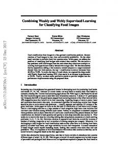
tive to its input parameter. Figure 2 shows the fairly consistent performance of self-training with seven or more bags for the MUC-6 data set. We observe similar trends for the MUC-7 data set. These results are consistent with empirical studies of bagging across a variety of classification tasks where seven to 25 bags are deemed sufficient (Breiman, 1996). To gain a deeper insight into the behavior of selftraining, we plot the learning curve for self-training using 7 bags in Figure 3, again for the MUC-6 data set. At iteration 0 (i.e. before any unlabeled data is incorporated), the F-measure score achieved by self-training is higher than that of the baseline system (58.5 vs. 55.5). The observed difference is due to voting within the self-training algorithm. Voting has proved to be an effective technique for improving the accuracy of a classifier when training data is scarce by reducing the variance of a particular training corpus (Breiman, 1996). After the first iteration, there is a rapid increase in F-measure, which is accompanied by large gains in precision and smaller drops in recall. These results are consistent with our intuition regarding self-training: at each iteration the algorithm incorporates only instances whose label it is most confident about into
80
tures causes the generative model and hence EM to perform poorly. Although self-training depends on the same model, it only makes use of the binary decisions returned by the model and is therefore more robust to the naive Bayes assumptions, as reflected in its fairly impressive empirical performance.5 In contrast, the fact that EM relies on the probability estimates of the model makes it more sensitive to the correctness of the model.
Baseline Recall Precision F−measure 75
Score
70
65
60
5 55
50
0
1 2 Number of Self−Training Iterations
3
Figure 3: Learning curve for self-training using 7 bags for the MUC-6 data set. the labeled data, thereby ensuring that precision will increase. 4 As we can see from Table 3, the recall level achieved by co-training is much lower than that of self-training. This is an indication that each co-training view is insufficient to learn the concept: the feature split limits any interaction of features in different views that might produce better recall. Overall, these results provide evidence that self-training is a better alternative to co-training for weakly supervised learning for problems such as coreference resolution where no natural feature split exists. On the other hand, EM only gives rise to modest performance gains over the baseline system, as we can see from row 4 of Table 3. The performance of EM depends in part on the correctness of the underlying generative model (Nigam et al., 2000), which in our case is naive Bayes. In this model, an instance with � feature values � ��
���� , ����� , and class � is created by first choosing the class with prior probability ������� and then generat ��
�"! ing each available feature with probability ��� ��� independently, under the assumption that the feature values are conditionally independent given the class. As a result, model correctness is adversely affected by redundant features, which clearly invalidate the conditional independence assumption. In fact, naive Bayes is known to be bad at handling redundant features (Langley and Sage, 1994). We hypothesize that the presence of redundant fea4
When tackling the task of confusion set disambiguation, Banko and Brill (2001) observe only modest gains from selftraining by bootstrapping from a seed corpus of one million words. We speculate that a labeled data set of this size can possibly enable them to train a reasonably good classifier with which self-training can only offer marginal benefits, but the relationship between the behavior of self-training and the size of the seed (labeled) corpus remains to be shown.
Meta-Bootstrapping with Feature Selection
If our hypothesis regarding the presence of redundant features were correct, then feature selection could result in an improved generative model, which could in turn improve the performance of weakly supervised EM. This section discusses a wrapper-based feature selection method for EM. 5.1 A Two-Tiered Bootstrapping Algorithm We now describe the FS-EM algorithm for boosting the performance of weakly supervised algorithms via feature selection. Although named after EM, the algorithm as described is potentially applicable to all single-view weakly supervised algorithms. FS-EM takes as input a supervised learner, a single-view weakly supervised learner, a labeled data set # , and an unlabeled data set $ . In addition, it assumes knowledge of the positive class prior (i.e. the true percentage of positive instances in the data) like co-training and requires a deviation threshold that we will explain shortly. FS-EM, which has a two-level bootstrapping structure, is reminiscent of the meta-bootstrapping algorithm introduced in Riloff and Jones (1999). The outer-level bootstrapping task is feature selection, whereas the inner-level task is to learn a bootstrapped classifier from labeled and unlabeled data as described in section 4. At a high level, FS-EM uses a forward feature selection algorithm to impose a total ordering on the features based on the order in which the features are selected. Specifically, FS-EM performs the three steps below for each feature %'& that has not been selected. First, it uses the weakly supervised learner to train a classifier ( from the labeled and unlabeled data ( #�)�$ ) using only the feature %'& as well as the features selected thus far. Second, the algorithm uses ( to classify all of the instances in #*)+$ . Finally, FS-EM trains a new model on just $ , which is now labeled by ( . At the end of the three steps, exactly one model is trained for each feature that has not been selected. The forward selection algorithm then selects the feature with which the corresponding model achieves the best performance 5 It is possible for naive Bayes classifiers to return optimal classifications even if the conditional independence assumption is violated. See Domingos and Pazzani (1997) for an analysis.
on # (w.r.t. the true labels of the instances in # ) for addition to ,�-/.�0 (the set of features selected thus far).6 The process is repeated until all features have been selected. Unfortunately, since # can be small, selecting a feature for incorporation into , -1.20 by measuring the performance of the corresponding model on # may not accurately reflect the actual model performance. To handle this problem, FS-EM has a preference for adding features whose inclusion results in a classification in which the positive class prior (i.e. the probability that an instance is labeled as positive), 3 & , does not deviate from the true positive class prior, 3 , by more than a pre-specified threshold value, 4 . A large deviation from the true prior is an indication that the resulting classification of the data does not correspond closely to the actual classification. This algorithmic bias is particularly useful for weakly supervised learners (such as EM) that optimize an objective function other than classification accuracy and can potentially produce a classification that is substantially different from the actual one. Specifically, FS-EM attempts to ensure that the classification produced by the weakly supervised learner weakly agrees with the actual classification, where the weak disagreement rate between two classifications is defined as the difference between their positive class priors. Note that weak agreement is a necessary but not sufficient condition for two classifications to be identical.7 Nevertheless, if the addition of any of the features to , -1.20 does not produce a classification that weakly agrees with the true one, FS-EM picks the feature whose inclusion results in a positive class prior that has the least deviation instead. This step can be viewed as introducing “pseudo-random” noise into the feature selection process. The hope is that the deviation of the high-scoring, “highdeviation” features can be lowered by first incorporating those with “low deviation”, thus continuing to strive for weak agreement while potentially achieving better performance on # . The final set of features, ,�5�&�-16"7 , is composed of the first 8 features chosen by the feature selection algorithm, where 8 is the largest number of features that can achieve the best performance on # subject to the condition that the corresponding classification produced by the weakly supervised algorithm weakly disagrees with the true one by at most 4 . The output of FS-EM is a classifier that the weakly supervised learner learns from # and $ using only the features in , 5�&�-16"7 . The pseudo-code describing FS-EM is shown in Figure 4. 6 The reason for using only 9 (instead of 9 and : ) in the validation step is primarily to preclude the possibility of getting a poor estimation of model performance as a result of the presence of potentially inaccurately labeled data from : . 7 In other words, ;=;/� does not imply that the corresponding classifications are identical.
Input:
(a supervised learning algorithm) (a single-view weakly supervised learning algorithm) 9 (labeled data) (unlabeled data) : A (original feature set) ; (true positive class prior) B (deviation threshold) A AJILKNM Initialize: CEDF