Modular robotics is the assembly of simple individual modules into a larger, ... For
the algorithm presented in this paper, the initial con- figuration has to be ...
Self-Reconfiguration Using Graph Grammars for Modular Robotics Daniel Pickem ∗ Magnus Egerstedt ∗ ∗
Georgia Institute of Technology, Atlanta, GA 30332 USA, {daniel.pickem,magnus}@gatech.edu
Abstract: In this paper, we apply graph grammars to self-reconfigurable modular robots and present a method to reconfigure arbitrary initial configurations into prespecified target configurations thus connecting the motions of modules to formal assembly rules. We present an approach for centralized reconfiguration planning and decentralized, rule-based reconfiguration execution for three-dimensional modular structures. The reconfiguration is done in two stages. In the first stage, paths are planned for each module and then rewritten into production rules as defined for graph grammars. In stage two, these rules are applied in a decentralized fashion by each node individually.We show that our approach yields a unique reconfiguration sequence and a graph grammar that results in the target configuration being the only reachable stable configuration. 1. INTRODUCTION Modular robotics is the assembly of simple individual modules into a larger, functional robot. The benefit of constructing such modular robots out of smaller building blocks is that they can be rearranged into different configurations that can perform different functions and have different capabilities. In fact, the key advantages of modular robots are their potential for versatility, robustness, and low cost. The ability to reconfigure allows modular robots to adapt to new tasks and environments by changing their morphology. Broken modules can be replaced by functional ones or new modules can be added without changing the general functionality of the structure (see for example Yim et al. [2007]). The goal of this work is to present a novel approach for the automatic reconfiguration of three-dimensional modular robots from an arbitrary initial configuration into a desired target configuration. This process is completed in two stages; the planning and the execution stage. In stage one, paths are planned for every module from its initial position to its target position. The resulting paths are then rewritten into a ruleset. This paper follows the general route laid down in Jones and Mataric [2003], where rules are automatically generated for two-dimensional structures. Three-dimensional structures were addressed in Brandt and Ostergaard [2004], albeit only for a much smaller class of systems compared to what is done in this paper. For the algorithm presented in this paper, the initial configuration has to be known (as is also the case for Jones and Mataric [2003] and Brandt and Ostergaard [2004]). The dependence on initial configurations has been treated in Fitch et al. [2003] for manually defined rulesets. Other work on manually defined rulesets includes Butler et al. [2004] who have demonstrated the feasibility and scalability of rule-based self-reconfiguration. The rulesets in these papers do not contain graph grammatical production rules. Klavins [2007], on the other hand, manually synthesizes graph grammars for two-dimensional reconfiguration and
we will follow the approach for three-dimensional structures in this paper. The main contribution of this paper is the automatic generation of graph grammars for the self-reconfiguration of three-dimensional structures. Any arbitrary initially connected configuration composed of cubic modules can be reconfigured into any prespecified target configuration. The only constraints of our method are that both configurations are not allowed to contain any enclosures and have to feature an overlapping region that contains at least one module. Our approach yields a unique reconfiguration sequence and we prove that the target configuration is the only possible outcome of the reconfiguration sequence. 2. RELATED WORK Much work has been done on the planning aspect of selfreconfiguration. This section specifically presents relevant rule-based reconfiguration approaches. Butler et al. [2004] describe a rule-based system inspired by cellular automata. Their rulesets are designed manually and enable groups of modules to split and merge, climb over or move around obstacles, or move through tunnels. Brandt and Ostergaard [2004] introduce a rule-based control strategy for the ATRON system (see Brandt et al. [2007]). Their rules take connectivity information into account and are automatically generated. They introduce wild card rules to reduce the size of the ruleset. Jones and Mataric [2003] show rulebased control for two-dimensional structures. The rules are automatically generated and only use connectivity information to check for rule applicability. These rules are either manually synthesized, limited to a specific class of structures or do not guarantee a successful reconfiguration to the target structure. Graph grammars, as a tool for manipulating graphs, have also been applied to modular robotics. Klavins [2007], for example, uses graph grammars to reconfigure programmable parts, a triangle shaped hardware implementation. He manually synthesizes rulesets that are designed to
form specific structures out of the triangular modules. As opposed to our system, Klavins [2007] allows multiple rules to be applicable to the whole system at the same time. Unlike for our system, this approach does not guarantee a uniquely determined reconfiguration sequence or the reaching of the target configuration.
3. SYSTEM REPRESENTATION In this paper we investigate a modular robotic system whose basic building blocks are visually represented by cubes (see Fig. 1). Moreover, no physical constraints beyond collision-avoidance such as gravity, module masses, or forces are taken into account. Additionally, the entire reconfiguration process happens in free space and is not restrained by walls, floors, or any other obstacles. These assumptions are made in order to focus the contribution on the self-reconfiguration process rather than on implementation-specific details. Following the taxonomy in Yim et al. [2007], modular robots can generally be categorized into lattice-type and chain-type architectures. We present a lattice-based system that is embedded in a discrete coordinate system using the sliding cube model (see Fitch et al. [2003]). In the sliding cube model, every module is represented as a cube with dimension δ (w.l.o.g. we use unit cubes, i.e. δ = 1), an origin xi ∈ Z3 , a globally unique integer identifier, and labels. A cube is capable of executing motions, which can be generally described as functions f (xi , m) = xi + m where xi ∈ Z3 and m ∈ Z3 . Therefore, a motion moves a cube to a new position in Z3 . In particular, the cubes in our system are capable of two primitive motions - sliding along a surface made of other cubes as well as transitioning to orthogonal surfaces. Definition 1. A sliding motion ms is such that f (xi , ms ) = xi + ms where xi ∈ Z3 and ms ∈ Z3 ∧ ms ∈ Ms . Ms is the set of all possible sliding motions and is defined as Ms = {m ∈ Z3 |mx = 1 ∨ my = 1 ∨ mz = 1 ∧ mx + my + mz = 1}. Definition 2. A corner motion mc is such that f (xi , mc ) = xi + mc where xi ∈ Z3 and mc ∈ Z3 ∧ mc ∈ Mc . Mc is the set of all possible corner motions and is defined as Mc = {m ∈ Z3 |mx < 2 ∧ my < 2 ∧ mz < 2 ∧ mx + my + mz = 2} 1 . Note, however, that we will not allow the application of sliding or corner motions unless they are feasible, i.e. obey connectivity constraints and do not collide with other cubes. In fact, the movement of individual cubes requires a connected substrate of other cubes, which is referred to as a configuration.The representable space of our system is Z3N and any configuration C is a subset of the representable space, C ⊂ Z3N . One way in which a configuration can be described is through three adjacency matrices and a labelset. Every adjacency matrix describes the adjacency of cubes along one dimension. Its entries are given by g(C) = (Ak , l), where 1 In Rus and Vona [2001], a corner motion is referred to as convex motion
1 Ak = [ai,j,k ] = −1 0
if (xi − xj )T · bk = 1 if (xi − xj )T · bk = −1 otherwise
l(i) = l(ci ), ci ∈ C, i, j ∈ {1, . . . , N } Here, k represents one dimension of the configuration space Z3N spanned by the three orthogonal base vectors bk , ci stands for a cube of the configuration C, and the labels l(i) of node i are the same as the labels of cube ci . One adjacency matrix for every dimension of the configuration space is required to encode the three-dimensional geometry of the configuration. Alternatively, a configuration can be represented as a labeled graph. Definition 3. The represented graph G = (V, E, lG ) is composed of the vertex set V , the edge set E, and edge and vertex label set lG and is derived from (Ak , l) via the adjacency-to-graph mapping (V, E, lG ) = h(Ak , l). V is a finite set of integers corresponding to the cube IDs, i.e. V = {1, . . . , N }, where N is the total number of cubes. E is derived from the three adjacency matrices Ak as E ⊆ V × V , with ei,j ∈ E if Ai,j,k 6= 0 for some k ∈ {1, 2, 3}. lG contains edge labels and vertex labels and is derived from Ak and l as follows: lG (vi ) = l(ci ) with vi ∈ V, ci ∈ C lG (ei,j ) = sign(Ai,j,k )bk with ei,j ∈ E and Ai,j,k 6= 0 Here, i, j ∈ {1, . . . , N }, l(ci ) ∈ l, and bk is a base vector. The vertex labels of vi ∈ G are the same as the labels for the cubes ci ∈ C. G is a directed, labeled graph that preserves the three-dimensional structural information of the configuration. The graph notation is required to define graph grammar rules and apply them to our system in Section 5.2. An advantage of the graph notation is that we can apply graph theoretical concepts such as the notion of connectivity. In this paper, we assume that the initial configuration C I and the target configuration C T are known and contain the same number of modules. We then employ a two-stage planning process, in which we plan paths for every module that has to be moved in stage one (see Section 4) and generate the ruleset based on these paths in stage two (see Section 5.2). The ruleset is then executed as shown in Section 5.3. 4. PATH PLANNING The reconfiguration process requires us to move cubes from their initial positions to their target positions. Therefore, we have to calculate paths for cubes ci ∈ C I to their desired positions in cj ∈ C T . Cubes ci in the initially overlapping region Oinit = C I ∩ C T (see Fig. 1(a)), do not have to be moved and are excluded from the planning process. The planning stage is composed of multiple steps, which are the calculation of the currently overlapping region O = C ∩ C T , the movable set M, the immediate target successor set R, the path calculation (for every cube ci ∈ C I \ Oinit ), and the ruleset generation (see Section 5.2). In this section, we will formally define M and R, the notion of articulation points and paths, and describe the planning approach. Definition 4. An articulation point v in a graph G is a node whose removal would increase the number of
(a) Initial configuration (transparent), target configuration (wireframe), and overlapping nodes (opaque)
(b) Movable nodes (opaque) as part of the initial configuration (transparent)
(c) Immediate target successor positions (opaque) as neighboring positions of the initial configuration (transparent)
Fig. 1. Graphical representation of the overlapping, movable, and immediate target successor set in the simulator connected components c(G), i.e. c(G − v) > c(G) 2 . In other words, the removal of v would disconnect the graph.
O) ∩ M to position cj ∈ C T ∩ R. The length of the path pi , or the total number of motions, is denoted as |pi |.
A connected graph G has only one connected component, c(G) = 1. Our self-reconfigurable system has to remain connected at all times to guarantee a successful reconfiguration. In order to enforce this requirement, we have to ensure that a node that is an articulation point is never moved. The movable set is therefore defined as follows: Definition 5. The movable set M is a set of cubes that can be moved without disconnecting the configuration and is defined as M = {ci ∈ C|ci ∈ C I \ O ∧ ci ∈ / A(C) ∧ |N1 (ci , C)| ≤ 5}. N1 (ci , C) is the one-hop neighborhood and defined as N1 (ci , C) = {cj ∈ C|dist(ci , cj ) = 1}. A(C) is the set of articulation points of the graph representing the current configuration C.
Both M and R define a set of cubes. Before we can plan a path for a cube ci to a position cj , we need to define an assignment. Therefore, we calculate the pairwise costs between any two cubes ci ∈ M and cj ∈ R and pick the pair of cubes with the lowest cost. The assignment resulting from this greedy approach is then used as input for the path planner. This process is repeated for all cubes ci ∈ C I \ O and paths are computed to their respective target positions cj ∈ C T . Note that this approach ensures that progress is never blocked and the target configuration will indeed be assembled given that the initial configuration is connected and does not contain any enclosures (see Theorem 1) In this paper, we use A* for path planning together with the Manhattan distance as cost metric as it most accurately represents the discrete lattice structure of our system and the possible movements of the nodes. The result of the path planning stage is a set of paths that describe the complete reconfiguration from C I to C T . This set of paths is then rewritten into a ruleset as discussed in the next section.
This definition is based on the sliding cube model (see Fitch et al. [2003]) and only allows modules on the surface of the configuration to be relocated. This is because Def. 5 excludes immobile cubes within the configuration (i.e. cubes that have six neighbors) from the movable set. While M is a set of movable cubes, we need to find potential target positions for cubes ci ∈ M - the immediate target successor set R. Definition 6. The immediate target successor set R is defined as positions cj ∈ C T that are adjacent to the current configuration, i.e. lie in the one-hop neighborhood N1 (C) of the current configuration C as well as in the target configuration C T . R = (C T ∩ N1 (C)) \ C, where N1 (C) = {cj |cj ∈ / C ∧ ci ∈ C ∧ dist(ci , cj ) = 1} (see Fig. 1(c)). Therefore, R is a subset of N1 (C). Note that N1 (C) is the one-hop hull of the current configuration C and at the same time the planning space for the path planner. In that planning space, we plan a path pi for a single cube at a time, i.e. from ci ∈ M to cj ∈ R. We know by assumption that R is nonempty unless the target configuration has already been assembled. The path pi is only allowed to contain positions ck ∈ N1 (C) and use primitive motions to move the current cube ci . Definition 7. A path is a concatenation of motions m ∈ {mc , ms } (see Def. 1 and Def. 2) that move cube ci ∈ (C I \ 2 Connected components of a graph G are its maximal connected subgraphs.
5. RULE GENERATION In this paper, we employ graph grammatical concepts to bridge the gap between global information that is available during planning and local information that is available to the cubes during reconfiguration. The centralized path planning results are rewritten into rules that can be checked locally for applicability. Contrary to rules only based on connectivity information, graph grammars offer fine-grained control over the applicability of rules and allow the encoding of additional information into the labels of the rules. Before we introduce our rule generation and execution approach, we define the graph grammatical terms used in this paper, taken from Klavins et al. [2006]. Definition 8. A production rule or simply a rule consists of two labeled graphs; a left-hand side gl and a right-hand side gr . It describes a transformation of a graph GS , that is isomorphic to gl , from GS to gr .
A graph grammar is a set of production rules that operate on a graph G0 . Therefore, we call the pair (G0 , Φ) a system, where G0 is an initial labeled graph and Φ is a graph grammar. A rule r ∈ Φ can be applied to G0 only when it is applicable: Definition 9. A rule is applicable to G if there exists a subgraph GS of G that is isomorphic to gl . This is also denoted as GS ∼ = gl . Once the applicability of a rule r to a subgraph GS of G has been determined, r can be applied to G. The application r of a rule r yields a new graph Gi − → Gi+1 , where Gi+1 results from Gi by replacing the subgraph GS with gr . Each step in the reconfiguration process yields a graph Gi that is part of a trajectory, i.e. a finite or infinite sequence σ = {Gi }ki=0 s.t. there exists a sequence of applicable rules ri → Gi+1 . Each graph Gi is {ri }k−1 i=0 where ri ∈ Φ and Gi − called reachable by the system (G0 , Φ). A reachable graph can be temporary, such that some rule r in Φ is applicable to it, or stable (see Klavins et al. [2006]). Definition 10. A graph G is stable, if no rule in Φ is applicable to it. Stable graphs play an important role in this paper. In this section, we prove that the graph representing C T is the only reachable stable graph given a system (G0 , Φ). Here, G0 is derived from C I and Φ is an automatically generated graph grammar. Furthermore, this section describes the structure of our rules and the rule generation framework. 5.1 Rule Structure For the purpose of self-reconfiguration, a production rule for our system uses the rule structure shown in Def. 8 and its two labeled graphs gl and gr are defined as follows: gl = f (N2 (ci , C))
(a) Left-hand side of a rule
(b) Right-hand side of a rule
Fig. 2. Visual representation of a rule showing a corner motion of cube 1. f −1 (gr ) of some rule. The highlighted cube is the currently active cube ci . As part of gl and gr , each rule contains information about how the labels of the current node change through the application of the rule as well as optional label updates for the neighbors. Each label is composed of multiple data fields, which include the node ID, the rule ID, a flooding flag indicating the start and the end of the flooding process, and a field storing the latest finished path. The node ID and the rule ID are globally unique integers and ensure the uniqueness of each rule and the unambiguity of the whole reconfiguration. The flooding flag controls the start and end of the propagation process to update every node’s knowledge about the latest finished path. The field last path concludes a label and stores the most recently finished path locally at every node. This field also controls the execution sequence of all individual paths, since the execution of path pi depends on the conclusion of path pi−1 . The initial labeling of all nodes of the graph G0 = (V, E, lG ) = f (C I ) and the label update mechanism through rules are designed so that only one rule is applicable to any cube vi ∈ V at any given time. Therefore, the reconfiguration is unambiguous and deterministic.
gr = f (N2 (ci + m, C)), f is given below but essentially maps from cubesets to graphs. N2 (ci , C) is the immediate motion successor set of the current cube ci in the configuration C and √ is given by N2 (ci , C) = {cj ∈ C|ci ∈ C ∧ dist(ci , cj ) ≤ 2}. N2 (ci , C) contains all cubes at a distance of one primitive motion from cube ci . Both graphs, gl and gr , are derived from the sets N2 (ci , C) and N2 (ci + m, C) of ci and its current motion m (given by the path planner) via the cubeset-tograph mapping f . Definition 11. The relationship between a cubeset C and a graph G = (V, E, lG ) is given by the cubeset-to-graph mapping f, which is defined as f = h ◦ g such that (V, E, lG ) = f (C) with mappings g and h defined in Section 3. The inverse graph-to-cubeset mapping f −1 is given by f −1 = g −1 ◦ h−1 such that f −1 (V, E, lG ) 3 C. ∼ The application of a rule r to a subgraph GS , i.e. r(GS = gl ) = gr , yields a new graph G0 . The changes in the edge r 0 and label set described by G = (V, E, lG ) − → (V, E 0 , lG )= 0 G represent the motion in the configuration space, i.e. C = f −1 (G) and C 0 = f −1 (G0 ), where ci has been moved from ci ∈ C to ci + m ∈ C 0 . Fig. 2 shows a graphical representation of N2 (ci , C) = f −1 (gl ) and N2 (ci + m, C) =
5.2 Rule Generation The main contribution of this paper is the automatic generation of a graph grammar Φ that describes the unamΦ biguous reconfiguration C I − → C T . The path planning and the rule generation are interleaved, which means that once a path pi (i ∈ {1..|P |} where |P | = |C I \ Oinit | = |C T \ Oinit |) has been computed, the ruleset Rpi that represents pi is generated. Rpi consists of |pi | motion rules, one flooding activation rule, and one propagation rule. More |pi | formally Rpi is defined as Rpi = {{rmi }i=1 , rp , rf }. The entire ruleset Φ is composed of all sub-rulesets Rpi , i.e. |P | Φ = {{Rpi }i=1 }. The three types of generated rules are defined as follows: Definition 12. A motion rule rm changes the edge set and the label set of the graph G = (V, E, lG ), specifically those edges whose end point is the current node vi . Therefore, the application of a motion rule results in the motion of a cube ci (represented by node vi ∈ G) in the configuration space C. More formally, rm rewrites the graph G = (V, E, lG ) as follows: r
0 (V, E, lG (vi )) −−m → (V, E 0 , lG (vi ))
Definition 13. A flooding activation rule rf updates the last path field of the current node vi and sets the flooding flag from 1 to 0, which activates the corresponding propagation rule. A flooding rule only affects the labels of the current node vi and does change the edge set. More formally, rf rewrites the graph G = (V, E, lG ) as follows: rf
0 (V, E, lG (vi )) −→ (V, E, lG (vi )) Definition 14. A propagation rule rp updates the current node vi ’s labels by setting the flooding flag from 0 to 1 and incrementing the last path field of all its neighbors vj ∈ f (N2 (ci , C)). It also sets the flooding flag of its neighbors vj to 0 so that the same rule rp is applicable to them. This type of rule is a wildcard rule w.r.t. the node ID. A propagation rule does not change the edge set. More formally, rp rewrites the graph G = (V, E, lG ) as follows: rp
0 (V, E, lG (vi , vj )) −→ (V, E, lG (vi , vj ))
For each motion mj in the path pi , the neighborhood structure of two consecutive positions of the active cube is calculated and stored in a rule. Additionally, each rule stores the labels before and after the application of the rule. More formally, for each motion mj (j ∈ {1..|pi |} as defined in Def. 7) of path pi , our algorithm generates a motion rule ri,j composed of gl and gr :
gl = f (N2 (ci + (
j X
mk ) − mj , C)
k=1
gr = f (N2 (ci +
j X
mk , C)
k=1
Here, ci is the currently moved cube and the starting point of path pi and N2 (ci , C) is the immediate motion successor set as defined in Section 5.1. The labels of gl are defined the following way: if j > 1 lG (gri,j−1 ) lG (gli,j ) = lG (gri−1,|pi−1 | ) if j = 1, i > 1 lG,init otherwise The labels of gr are derived from the labels of gl via the label update mechanism defined for motion rules, flooding rules, and propagation rules and can be summarized as follows. rm lG (gli,j ) −−→ lG (gri,j ) for motion rules rf lG (gri,j ) = lG (gli,j ) −→ lG (gri,j ) for flooding rules rp lG (gli,j ) −→ lG (gri,j ) for propagation rules The labels are created with a strictly monotonically increasing global rule ID ensuring that each rule is globally unique and describes exactly one step in the complete reconfiguration sequence. This process is repeated for every motion mj of path pi . After the end of the current path pi is reached a flooding activation rule and a propagation rule are generated, |pi | resulting in a ruleset Rpi = {{rmi }i=1 , rp , rf }. The rule generation process is repeated for every path pi (i ∈ {1..|P |}) until the reconfiguration is completed, i.e. until the target configuration C T has been assembled. This means that the only reachable, stable graph as defined
in Def. 10 is the graph representing the desired target configuration C T . Theorem 1. The graph G = (V, E, lG ) = f (C T ) representing the target configuration C T is the only reachable, stable graph to the ruleset Φ. Proof 1. This proof is based on Theorem 1 in Rus and Vona [2001] and the definition and properties of a unitmodular self-reconfiguring system. Our system is composed of unit cubes, which can be assembled into arbitrarily shaped configurations. Thus our system satisfies property one. Property two states that in a configuration composed of unit modules, there always exists a module that can be relocated to any position on the surface S. In our system, S is defined as S = N1 (C) = {ci |ci ∈ / C∧ cj ∈ C ∧ dist(ci , cj ) = 1} and R is a subset of S, R ⊂ S. The movable set M, on the other hand, is a subset of the boundary ∂C of C, where ∂C = {ci |ci ∈ C ∧ |N (ci , C)| ≤ 5}. |M| ≥ 2 according to Lemma 6 in Rus and Vona [2001] and only contains cubes ci ∈ ∂C. Therefore, our system fulfills property two of Theorem 1 as well. As a result, our system is self-reconfigurable and C T can be assembled incrementally from C I . Therefore, every cube ci ∈ C I \ Oinit will be moved to its target position cj ∈ C T . Since the current configuration C always remains connected (by construction of M and R), i.e. c(G) = c(f (C)) = 1, a path always exists between ci and cj . The individual module paths are planned sequentially, which means that path pi+1 is planned after path pi was planned and executed. This approach implicitly determines a unique reconfiguration sequence.The outcome of the planning stage, i.e. the execution of paths pi for i ∈ {1, . . . , N } with N = |C I \ Oinit |, therefore, unambiguously yields C T . By construction of the ruleset and the label update mechanism, the same sequence of reconfiguration steps is achieved during the execution stage of the ruleset. Therefore, we can conclude that the only reachable, stable graph is (V, E, lG ) = f (C T ). 2 5.3 Ruleset Execution The goal of the ruleset execution is the reconfiguration of C I into C T . In other words, given a system (G0 , Φ) we want r1 r2 r3 to execute the assembly sequence G0 −→ G1 −→ G2 −→ rn . . . −→ Gstable , where G0 = f (C I ), Gstable = f (C T ), and n is the total number of rules. To accomplish this reconfiguration, every node vi ∈ G periodically checks the ruleset for applicable rules r ∈ Φ. If the graph represented by the current neighborhood N2 (ci , C), i.e. GS = f (N2 (ci , C)) is isomorphic to the left-hand side gl of some rule r ∈ Φ, an applicable rule has been found and is applied to the current node vi . The application of r a rule r rewrites the subgraph GS into gr , i.e. GS − → gr . If the application of a rule changes the edge structure of GS , which is the case only for motion rules, the cube ci is moved in the configuration space. The execution of the last motion rule rmi,|pi | of a path pi triggers a flooding activation rule rfi . This rule in turn triggers a propagation rule rpi . Through the repeated application of rpi to every node vi ∈ V every node’s local state is updated about the completion of the latest path through directed flooding. This process is repeated until every path pi is completed and no more rules in Φ are applicable to any node vi ∈ V ,
Table 1. Reconfiguration planning results for overlapping box configurations Size
Overlap [N]/[%]
Steps
Rules
Runtime [min]
100
30 / 30%
837
907
3.70
200
60 / 30%
1543
1683
16.65
300
90 / 30%
2426
2636
63.26
400
120 / 30%
3279
3559
135.64
500
150 / 30%
4275
4625
246.93
250
4000
150
3000
100
Ruleset size [N]
Runtime [min]
200
Runtime [min] Ruleset size [N] Cubic approximation for runtime Linear approximation for ruleset size
2000 50
1000 0 100
150
200
250 300 350 Configuration size [N]
400
450
500
Fig. 3. Number of generated rules and required runtime for ruleset generation of box configurations i.e. until a stable graph is reached. An example of a reconfiguration sequence is shown in Fig. 4. 6. RESULTS This section presents simulation results obtained by reconfiguring overlapping box configurations (see Table 1), which ranged in size from 100 to 500 modules. Our test system was equipped with an Intel Core i5-540M dual core processor and 4GB of DDR3 memory. In Table 1, the field Size refers to the number of modules in the configuration, Overlap is the number of initially overlapping modules, Steps is the total number of motions of all modules to achieve the desired reconfiguration, Rules is the total number of generated rules in the ruleset, and Runtime is the time it took to generate the ruleset. As shown in Fig. 3, the size of the ruleset increases approximately linearly with the number of nodes, while the runtime of our algorithm increases approximately cubically for the box configurations. The runtime is primarily determined by the planning approach, which necessitates planning a path for every individual node. Our algorithm features a time complexity of O(N 2 ) for the relocation of an individual cube and a total time complexity of O(N 3 ) for the entire reconfiguration process. REFERENCES D. Brandt, D. J. Christensen, and H. H. Lund. Atron robots: Versatility from self-reconfigurable modules. In In Proceedings of the IEEE International Conference on Mechatronics and Automation (ICMA), pages 2254– 2260, Harbin, China, Aug. 2007. David Brandt and Esben H. Ostergaard. Behaviour subdivision and generalization of rules in rule-based control of the atron self-reconfigurable robot, 2004.
Fig. 4. Example of a reconfiguration sequence from a random two-dimensional configuration to a chair. Zack Butler, Keith Kotay, Daniela Rus, and Kohji Tomita. Generic decentralized control for lattice-based selfreconfigurable robots. The International Journal of Robotics Research, 23(9):919–937, 2004. R. Fitch, Z. Butler, and D. Rus. Reconfiguration planning for heterogeneous self-reconfiguring robots. In Intelligent Robots and Systems, 2003. (IROS 2003). Proceedings. 2003 IEEE/RSJ International Conference on, volume 3, pages 2460 – 2467, Oct. 2003. Chris Jones and Maja J. Mataric. From local to global behavior in intelligent self-assembly. In Proceedings of the 2003 IEEE International Conference on Robotics and Automation, ICRA 2003, September 14-19, 2003, Taipei, Taiwan, pages 721–726. IEEE, 2003. E. Klavins. Programmable self-assembly. Control Systems, IEEE, 27(4):43 –56, Aug. 2007. E. Klavins, R. Ghrist, and D. Lipsky. A grammatical approach to self-organizing robotic systems. Automatic Control, IEEE Transactions on, 51 Issue: 6:949 – 962, 2006. Daniela Rus and Marsette Vona. Crystalline robots: Self-reconfiguration with compressible unit modules. Autonomous Robots, 10(1):107–124, Jan. 2001. Mark Yim, Wei-Min Shen, Behnam Salemi, Daniela Rus, Mark Moll, Hod Lipson, Eric Klavins, and Gregory S. Chirikjian. Modular self-reconfigurable robot systems – challenges and opportunities for the future. IEEE Robotics and Autonomation Magazine, March:43–53, 2007.