Department of Computer Science, University of Colorado,. Boulder ...... ment systems introduced by Habel and Kreowksi [3,4], with one technical change.
JOURNAL
OF COMPUTER
AND
SYSTEM
Edge-Label
SCIENCES
40, 188-228
Controlled
(1990)
Graph Grammars*
MICHAEL G. MAIN Department of Computer Science, University of Colorado, Boulder, Colorado 80309 AND
GRZEGORZ ROZENBERG Instirute of Applied Mathematics and Computer Science, University of Leiden, Leiden, The Netherlands; and Department of Computer Science, Univeristy of Colorado, Boulder, Colorado 80309 Received
March
22, 1988
We introduce a graph-grammar model based on edge-replacement, where both the rewriting and the embedding mechanisms are controlled by edge labels. The general power of this model is established-it turns out to have the complete power of recursive enumerability (in a sense to be made precise in the paper). In order to understand where this power originates, we identify three basic features of the embedding mechanism and examine how restrictions on these features affect the generative power. In particular, by imposing restrictions on all three features simultaneously, we obtain a graph-grammar model that was previously introduced by Kreowski and Habel. fi? 1990 Academic Press, Inc.
1. INTRODUCTION In recent years, node-label controlled (NLC) graph grammars have been intensively studied as a method for generating node-labeled graphs [l, 7-10, 133. The key feature of NLC-grammars is that both the rewriting of a subgraph and the embedding of a newly introduced subgraph are controlled by node labels. (This is in contrast to the algebraic approach [2], where rewriting and embedding are based on structural properties of graphs.) Node-labeled graphs, which are the subject of NLC-grammars, are fundamental objects with numerous applications in computer science and other areas. Within the realm of graphs, one also has edgelabeled graphs, which are equally fundamental. It is natural to ask how the labelbased control mechanism carries over to edge-labeled graphs. The aim of this paper is to initiate systematic research in this area. * G. Rozenberg has been supported in part by National Science Foundation Grant MCS-83-05245. M. Main has been supported in part by National Science Foundation Grant DCR-84-02341. 188 OO22OOOO/90 $3.00 Copyright All rights
0 1990 by Academic Press, Inc. 01 reproduction in any iorm reserved.
189
EDGE-LABELCONROLLEDGRAPHGRAMMARS
The model of edge-label controlled (ELC) graph grammars we are presenting is influenced by our experience with NLC-grammars, and by the research of H. J. Kreowski on edge replacement systems [3,4]. However, we should warn that making a proposal for ELC grammars involves much more than simply taking the dual of NLC grammars. The paper begins by presenting our basic ELC model and illustrating its features by examples. It turns out that our basic model is “too powerful” in the sense that it generates all the class of recursively enumerable graph languages. In order to formally state and prove this result, we have to formalize the notion of a recursively enumerable graph language. We do this by introducing a simple algorithmic language for constructing graphs. In analyzing ELC grammars more closely, one can distinguish three basic parameters used in the rewriting process. Roughly speaking, the first parameter determines whether neighboring edges can be deleted when an edge is rewritten. The second parameter determines whether the source and target nodes of a rewritten edge can “merge” during the rewriting process. The third parameter controls whether multiple copies of the source and target nodes of a rewritten edge can appear. We investigate the impact of these three parameters. It is interesting to notice that if we make all three parameters “restrictive,” then we get the original edge-replacement systems proposed by Habel and Kreowski [3,4]. Other combinations of the parameters yield other classes of languages. Terminology and notation. Throughout the paper, the term graph refers to a directed, edge-labeled, finite graph with at least one node (and with no self-loops). Multiple edges between the same pair of nodes are allowed. For a finite alphabet A, the set of all graphs with labels chosen from A is denoted G,. Formally, such a graph is a tuple (I’, E, 1, source, target), where V is a non-empty finite set of nodes, E is a non-empty finite set of edges, 1: E -+ A is a function assigning labels to edges, and source, target: E + V are functions assigning source and target nodes to edges. We do not distinguish between isomorphic graphs, so that the term “graph” actually refers to a class of isomophic graphs. The graph with exactly one node is denoted by ??. An edge labeled by A is called an A-edge. We say that an edge is incident to its source and target nodes, and two edges which are incident to a common node are called adjacent. Similarly, two nodes which are incident to a common edge are called adjacent. The set of nodes of a graph c( is denoted by nodes(u) and the set of edges of a is denoted by edges(a). The cardinality of a set S is denoted by ISI.
2. EDGE-LABEL CONTROLLED
GRAPH
GRAMMARS
DEFINITION 2.1. An edge-label controlled graph grammar
5-tuple (Z, A, P, S, C), where -
C is a finiteset of edge labels.
(ELC grammar) is a
190
MAINANDROZENBERG
- A is a proper subset of C, called the terminal labels; elements of 2’-- A are nonterminals. -
P is a finite set of productions; each production
has the form
where A is a nonterminal label, CIE G,, and LX,,,,,, and atargetare nonempty subsets of nodes(u). -
S is a nonterminal label called the start label.
-
CE (C v {ISOLATED}) x C is the connection relation.
An ELC grammar without a specified start label is called an ELC grammar scheme. The way that an ELC grammar generates a set of graphs (its graph language) is similar to the mechanism of node-label controlled (NLC) graph grammars, with the connection relation determining how a newly introduced subgraph is connected to the rest of the graph during a derivation step. The symbol ISOLATED in the domain of the connection relation is not in C. It is needed so that isolated nodes in a newly introduced subgraph can have new edges attached to them during a derivation step. But before the complete description of this mechanism, we need a short discussion of the productions. The graph CI,on the right side of a production, is nonempty since G, contains only nonempty graphs. These graphs are called daughter graphs, and intuitively a rule such as A := (CI,CI,,,,,, atarget) will be used to replace an A-edge by the subgraph a. In this replacement procedure, the labels of edges adjacent to various nodes in a will be important. For this reason, we assign a “type” to each node in a daughter graph, based on the labels of the node’s adjacent edges. These types are not an intrinsic part of the graph (i.e., the nodes remain unlabeled), but merely an aid in describing the replacement procedure. The “type” of a node with no incident edges is an ISOLATED-node.A node with an incident A-edge is an A-node. A node with several incident edges may have several types; for example, a node could be both an A-node and a B-node if it has both A and B edges incident to it. Throughout the replacement procedure, new edges will be added, connecting a daughter graph to the rest of the graph. But when we add these new edges, we will not change the “types” that we have identified with each node-i.e., if we add an A-edge, this will not make new A-nodes. The dependence of “types” on edge-labels is part of the philosophy behind ELC grammars. Our general guideline is that the entire ELC replacement procedure should depend on edge labels-in the same way that the NLC replacement procedure depends on node labels. This replacement procedure consists of two steps: rewriting an edge with a production rule that introduces a new subgraph, and embedding the new subgraph by adding new edges. The types will be used in the embedding step, and because of our underlying philosophy these types must depend on edge labels. Now we can give the complete description of the replacement procedure. Let
EDGE-LABEL CONROLLED GRAPH GRAMMARS
G = (Z; d, P, S, C) be an ELC grammar. A production is used to transform a graph in the following way.
191
A := (a, 01,,,,,, atarget) of P
Part 1. Start with a graph p; within p, choose any occurrence of an A-edge, which we will call the mother edge. Let s be the source node of the mother edge, and let t be the target node. All edges which are incident to s or t (except the mother edge) are called neighborhood edges. The mother edge, the neighborhood edges, plus s and t are now deleted from the graph ,u, yielding a new graph ,B’. Part 2. Add a copy of CI(the daughter graph) to the graph p’ (where the edges and nodes of the copy of a are disjoint from ,u’). Part 3. Now we introduce new edges between $ and the daughter graph. The introduction of these edges is controlled by the connection relation C, and by the “types” of the nodes in the daughter graph. The process consists of adding edges, according to one of the following rules:
(where u # t) (i) Outgoing edges. For each neighborhood egde +-%. and each node v E asource, if there is some Y such that v is a Y-node kd (Y, Z) E C, then connect v to u with a Z-edge (G J. Similarly, for each neighborhood Au (where u # s) and each node v E atarget, if there is some Y such that v edge , is a Y-node and (Y, Z) E C, then connect v to u with a Z-edge (GU). (ii) Incoming edges. For each neighborhood edge .-%. (where u#t) and each node v E Al__ if there is some Y such that v is a F-nodesand (Y, Z) E C, then connect u to v with a Z-edge (UA ,). Similarly, for each neighorhood edge L (where u #s) and each node v E atarget, if there is some Y such that v is a G-node and ( Y, Z) E C, then connect v to u with a Z-edge (U&V ). Part 4. The final thing that remains to be done is to establish some new internal edges in the daughter graph; these edges correspond to edges that were oiiginally parallel to the mother edge. Specifically, for each neighborhood edge I, and each pair of nodes u E CX,,,,,, and v E atarget, if there are two pairs (Y, Z) E C and (Y’, Z) E C such that u is a Y-node and v is a Y-node, then connect u to v with a Z-edge (UA ,). Similarly, for each neighborhood edge e s and each pair of nodes u E utarget and v E c(,,,,,, , if there are two pairs (Y, Z) E C and (Y’, Z) E C such that u is a Y-node and v is a Y’-node, then connect u to v with a Z-edge cU& ,). Since self-loops are not allowed, these connections are only done when u # v.
The final result has been to replace the mother edge with a copy of CLEdges were transferred from the mother’s source and target to tl,,,,, and atarget. Let q be the graph resulting after Part 4. We write p aG q to denote the relation “9 is directly derived from .Hin G.” If there exists a finite sequence of transformations,
192
MAIN AND ROZENBERG
then we write pc, *E p,,, and say that p,,, is derivedfrom p,, in G; the finite sequence is called a derivation of length m, and each application of the replacement procedure is one derivation step. The language generated by the grammar G, also called an ELC language, is the set of all graphs in G, which can be derived from a graph with a single S-edge connecting two nodes; that is,
Any graph which can be derived from the start graph +% is called a graphical from the context, the notation will be simplied to * and a*
form of G. Whenever the grammar G is understood
Examples
We present several examples of productions and their application in a replacement procedure. The nodes of a daughter graph CIwill be represented as follows: 0 is a node which is in neither ~~~~~~nor ~~~~~~~ ; 0 is a node which is in only asource; ? ?is a node which is in only atarget; and ? ?is a node which is in both GI,,,,,, and a target. EXAMPLE 2.1. Consider a grammar with one terminal b and one nonterminal B, and the complete connection relation (all of (6, B, ISOLATED} x {b, B} ). Here is a production rule that will can change a B-edge to a b-edge:
B:=
Q
bs
When this production is applied to a graph, the first part of the replacement procedure will select some B-edge as the mother edge. In Part 1 of the replacement procedure, this edge will be removed, along with its source, target, and neighborhood edges. This step would look like this for a typical graph (the mother edge is indicated by the dotted box): b
-0
Initial Graph
B
After Part 1
In Part 2 of this example replacement, a copy of the daughter graph is added. This yields the graph:
EDGE-LABEL CONROLLED GRAPH GRAMMARS
1YJ
b
-0
-0
b
B
After Part 2
For Part 3 of this example, new edges are established between the new daughter graph and the rest of the graph. Because the connection relation is the complete relation, this step is easy: each neighborhood edge is reestablished with a connection to the daughter’s source or target. The result is this graph:
After Part 3 EXAMPLE 2.2. Consider a grammar with the connection relation {(6, A), (X, a), (X, b)} and the following production (among others):
Let c1 be the right side of the above production. Here is an example of how the production is used in a replacement procedure. The example begins with the following four-node graph-the mother edge for this example is indicated by the dotted box. a
194
MAIN AND ROZENBERG
In Part 1 of the replacement procedure, the mother edge is removed, along with its source, target, and neighborhood edges. In this case there are four neighborhood edges (the two curved edges which are adjacent to the mother target and the two b-edges which are adjacent to the mother source). When these are removed, only a single edge remains, from the top of the previous drawing:
In Part 2 of the replacement procedure, a disjoint of the daughter graph is added, yielding this disconnected graph (the dotted line indicates the new daughter graph):
Also in Part 2 of the replacement procedure, we assign “types” to the nodes of the daughter graph, according to the labels of the adjacent edges. In this case, the upper node of the daughter graph is an X-node and a b-node; the lower left node is a b-node and an A-node; and the lower right node is an A-node and an X-node. In Part 3 of the replacement procedure, edges are established between the daughter graph and the rest of the graph. These edges are established by examining the connection relation, and by examining each of the neighborhood edges that were deleted in Part 1. For example, the pair (b, A) is in the connection relation, and there is a neighborhood A-edge from the mother target to the upper left node of the original graph. This implies that a new A-edge is established from every type b-node in atarget to the upper left node of the original graph. This gives one new edge:
...
Notice that there is no A-edge from the second node of atargetto the upper left node of the graph, since this second node is not a type b-node. In all, Part 3 will add four
EDGE-LABEL CONROLLED GRAPH GRAMMARS
195
edges between the daughter graph and the rest of the graph. At the end of Part 3, the graph looks like this: a
In this case, Part 4 does nothing (since there were no edges parallel to the mother edge), so the entire replacement procedure looks like this:
~
I-:“_:... i... :.............i *
EXAMPLE 2.3. Consider the same production as the previous example, but suppose that the connection relation contains only the pair (A, a). The production can be applied to the same graph as before, but the result is different. In particular, the daughter graph is reconnected to the rest of the graph in a different way. The pair (A, a) is in the connection relation, and there is a neighborhood u-edge from the upper right node of the original graph to the mother target node. Therefore a new a-edge is established from the upper right node of the original graph to every type A-node in atarget. The complete replacement procedure is drawn below, with the mother edge and daughter graph outlined: a
a
EDGE-LABEL CONROLLED GRAPH GRAMMARS
197
daughter graph (GI)which is in both CI,,,,,, and utarget. The connection relation for this example contains all possible pairs, and the production rule is:
EdLo
x :=
When this production is applied to an X-edge, a new X-edge is introduced, and all connections to the old X-target node are transferred to the new X-source node. Here is an example replacement procedure with the mother edge and daughter graph outlined:
A
...... . . ... . . . :
x
f
:................... .......
.................. :
:.‘.”
x
3
;
i . ..................... B
B
+:
+?
EXAMPLE 2.6. This is an example of a complete grammar. The nonterminal labels are {S, X, A}, with start label S. There are two terminal labels {a, b}. The connection relation is {(a, a), (a, A), (a, b), (6, A), (X, a), (X, b)}. There are these three productions (The source and target nodes for the daughter graph of the first production are not indicated because they are irrelevant; this production is only applied as the first step of a derivation, where there are no neighborhood or parallel edges.):
s :=
198
MAIN AND ROZENBERG
A derivation in this grammar begins by replacing the start label with the first production rule: A
At this point in the replacement procedure, the graph has precisely one X-edge, and two A-edges. The X-edge may be replaced using the second production rule, which will keep the total number of X-edges at one and add one new A-edge in a particular way. For example, applying the second production rule to the above graph results in this replacement procedure: A
The third production rule changes an A-edge to an a-edge. Because of the connection relation, an application of the third production also causes any X-edge adjacent to the mother source or target to “disappear.” This is because (a, X) is not in the connection relation. For example, here is a replacement procedure using the third production rule: A
a
This particular derivation can be completed by applying the third production rule to the remaining two A-edges. This gives the final two steps of the derivation like this:
EDGE-LABEL
CONROLLED
GRAPH
GRAMMARS
199
a
More generally, a derivation in this example grammar has these three stages: 1. The first derivation production rule.
step where the start-edge is replaced using the first
2. Applications of the second and third production rules, without replacing the A-edge adjacent to the X-edge. At each point in this stage, the graph has the form:
The edges around the “rim” are all labeled by either A or a. The only restrictions are that the edge which is immediately counterclockwise from X is an a-edge, and the edge which is immediately clockwise from X is an A-edge. 3. Eventually, in any derivation, the A-edge which is adjacent to the X-edge will be rewritten to an a. At this point, the X-edge disappears, since (a, X) is not in the connection relation. 4. The remainder of the derivation replaces any remaining A-edges with a-edges, using the third production rule. The end result is a graph of this form:
From this, it is easy to see that the grammar generates all graphs of the above form, with at least three a’s. In Section 8, we will show that this graph language cannot
200
MAIN AND ROZENBERG
be generated without a connection relation which breaks some edges (such as the way the X-edge is broken by replacing the adjacent A-edge). EXAMPLE 2.7. This is an example of a grammar which generates only discrete graphs. (There are no terminal labels.) The source and target sets for the productions of this grammar are always distinct single nodes of a daugther graph. Despite this simple form for productions, the grammar is interesting because the only graphs it generates have exactly 3 x (gn) nodes. This “exponential growth” in graph size will be used in Section 8. The start label for the grammar is S and the other nonterminal labels are (4, A,, A,, X B}. Th e connection relation contains these pairs:
(A,, Ai) for i=O, 1 or 2 Vi+,> Ai) for i = 0, 1 or 2; addition is modulo 3 (4 AZ) (ISOLATED,B).
Here are the productions of the grammar. As in the previous example, the source and target nodes of the first production are omitted, since this production is only used at the start of a derivation, s :=
---x---O
Ao
So
X
8 Ai :=
X
0
B:=
8
g%
There is no production for the non-terminal X-which means that the only way that an X-edge can disappear from a graph during a derivation is by replacing an adjacent edge and failing to reconnect the X-edge. Since there are no terminal labels, the grammar generates only discrete graphs. As mentioned above, the sizes of these discrete graphs are growing exponentially.
EDGE-LABEL CONROLLED GRAPHGRAMMARS
201
To prove this, let S*a, * ... *a,,, be a derivation of a discrete graph a,. We prove four properties which hold for any of the graphical forms ak: 1. Every non-X-edge in elk is adjacent to every other non-X-edge. 2. Every non-X-edge in c(~ is adjacent to one X-edge, and this X-edge is not adjacent to any other edge. 3. Let A:(Q) be the number of &-edges in Q, and similarly for A:, and B#. If elk contains at least one Ai-edge, then B#(Q)).
Inodes(g,)l =3x (A,#(a,)+Af(cr,)+A:(~l~)+ 4.
AT,
Define the value of Q to be the following integer: If A,#(a,) = 0 then value(cr,) = 9A F(Q) + ~A~#(cQ)+ lnodes(a,)l elsevalue(cck)=21A,#(cr,)+9Af(cc,)+45Af(a,)+
Inodes(a,)l.
Then there exists an integer n such that value(cl,) = 3 x (sn). The proof of these propertiy is byA6nduction on k. The base step (k = 1) is easy w and properties 14 are easily verified for since ~1~is the fixed graph this graph. The induction step is a case analysis, based on the five possible productions which can be applied at elk~ , = ctk. The fourth property implies that every graph generated by this grammar has 3 x (sn) nodes for some n. In fact, any such graph (n > 1) can be generated by this grammar. ??
3. EXPLICITELC GRAMMARS In order to use an ELC production, we associate “types” with each node of the daughter graph. These types are the labels of the edges which are incident to the node, and these types are used (in Parts 3 and 4) to determine which new connections are made between this node and the rest of the graph. Thus, the labels in daughter graphs serve two purposes: they label the edges, and they also control the “types” that affect the new connections. It may sometimes be convenient to separate these two roles of the edge labels. As an alternative to this method of associating types, we could explicitly assign types to the nodes of each daughter graph-without regard to the labels of incident edges. In particular, we could assign a set of edge labels L(U) to each node u of each daughter graph. If L(U) is the empty set, then u is to be treated as if it is an IsOLArED-node. Otherwise it will be treated as an A-node for each A in L(U). This explicit assigning of types to daughter graph nodes permits a simplier design of grammars in many cases. We call these grammars explicit ELC grammars (since each node of each daughter graph has an explicit set of labels assigned to it).
202
MAIN AND ROZENBERG
The formal definition of an explicit ELC grammar is the same as Definition 2.1, except that each production has the form
where L is a function from nodes(a) to 2= (the powerset of the edge label set). The four parts of the replacement procedure are unchanged, except that the “type” of a node v in the daughter graph is explicitly given by L(v). Can explicit ELC grammars generate graph languages which cannot be generated by any ELC grammar? No! The following theorem shows how an explicit ELC grammar can be converted to an ordinary ELC grammar, without affecting the language that is generated. THEOREM 3.1. The class of languages generated precisely the class of ELC languages.
by explicit ELC grammars
is
Clearly every ELC language can be generated by an explicit ELC gramProof mar. For the other direction, let G = (C, A, P, S, C) be an explicit ELC grammar. We will construct an ELC grammar G’ which generates the same language as G. The label set of G’ is C u P(Z), where P(Z) is the powerset of Z. The terminals are still A and the start symbol is still S. The productions of G’ are the same as those in G, but each daughter graph is modified. For each node u in a daughter graph, we add one extra node m,, and there is an edge labeled by L(u) from m, to U. The source and target subsets of the daughter graph remain unchanged. For each new nonterminal label XE P(Z), there is also one new production: X := ? ? . Finally, the connection relation of G’ is the union of these five sets:
{W, A)IXEp(n
andforsomeBEX:(B,A)ECj
{(0, A) I (ISOLATED,A) E C} {(ISOLATED,A)(A EC} {(X
Y)IX
YEPO)}
{(ISOLATED,X)IXE
P(C)}.
Each production of a derivation in G can be simulated in G’ by a sequence of productions: the first production corresponds to the step from G, but with the extra nodes m,, and the rest of the productions in the sequence apply the new productions to get rid of the m, nodes, by collapsing them into other nodes. In this way, each graph generated by G is also generated by G’. It is straightforward to show that these are the only graphs G’ generates. 1 The explicit form is useful for showing that specific languages are ELC. In particular, we will use it to show that ELC languages have the complete power of recursive enumerability. But first we must define R.E. graph languages, which is the subject of the next section.
203
EDGE-LABEL CONROLLED GRAPH GRAMMARS
4. RECURSIVELY ENUMERABLE GRAPH LANGUAGES This section defines recursively alphabet
A. Intuitively
these
enumerable are
graph languages
languages
whose
over a fixed terminal
elements
can
be effectively
enumerated. 4.1. Linear Descriptions of Graphs We start with a small “algorithmic graphs,
language”
using a simple set of primitive
which can be used to construct
instructions.
The instructions
allow opera-
tions like “add a new node” or “connect two specific nodes with a Y-edge.” The language is designed with one goal in mind: sequences of instructions should be easy to “simulate” allowable
by a fixed ELC
instructions
grammar.
Because
may not be the most natural
of this goal, the collection
possible,
enough to construct any graph (with 2 or more nodes). Each sequence of instructions can be thought of as a little algorithm a graph.
At the beginning
(before
any
graph” has exactly two nodes, labeled some edges, or nodes, assume
instructions
that the nodes
are labeled
by consecutive
keep track of one distinguished
node number
current = 1). As will be shown,
instructions
also renumber
are executed),
to generate the “current
1 and 2, and no edges. Each instruction
or does some other alteration
LEFT and RIGHT. The RIGHT instruction
adds
to the graph. At each step we integers
starting
can change
at 1. Also, we
called current (initially
in a variable
the value of current, and
the nodes. We begin with a list of the different instructions,
specify how they can be put together
of
but the set is complete
and then
to form “graph programs.”
The LEFT instruction
subtracts
one from the value of current.
adds one to the value of current.
EDGE, (Y is any label).
This
connects
node
number
current to node number
current + 1, using a Y-edge. SWAP.
This instruction
node number ADD.
This
swaps the node numbers
of node number
current with
current + 1. The value of current remains unchanged. instruction
adds
a new
node.
The
number
of the
new node
is
current + 1. Any node with a number higher than current has its node number incremented by 1. The value of current remains unchanged. JOIN.
This instruction
causes two nodes to merge. In particular,
bered current and current + 1 are joined disappear. Any other node number decremented by 1.
together.
with a number
higher
SKIP, IGNORE, and END. The SKIP instruction tion causes the next instruction to be ignored.
the nodes num-
Any edges between the two nodes than
current + 1 has its node
does nothing. The IGNORE instrucis a special instruction which
END
must appear twice at the end of each sequence. It has no effect on the construction of the graph. The “operational” reason for these instructions will become apparent later.
571/40/Z-6
204
MAIN AND ROZENBERG
These instructions can be put together sequentially to form “graph programs.” We require these programs to meet certain restrictions. In particular, RIGHT and EDGE, can only be given if current is less than the number of nodes in the current graph. A LEFT instruction requires current > 1, and the IGNORE instruction cannot be the final instruction in the algorithm, nor can it precede another IGNORE instruction. Also, we require that the total number of nodes in the graph being constructed is never less than 2-hence JOIN cannot appear unless there are at least three nodes in the graph. For reasons to be explained later, we also require that the SWAP and JOIN instructions appear only when current is less than n - 1 (where n is the number of nodes in the current graph). Finally, the END instruction must twice appear at the end of the sequence, and nowhere else. When these END instructions occur, the value of current must be 1. A graph program is any sequence of instructions which meet these rules. It is decidable whether a given string is a graph program: simply execute the potential program to see if any of the conditions are violated. Since program is straight-line code (no iteration/recursion) any potential program will eventually terminate or violate a condition. EXAMPLE.
Here is an example graph program: EDGE,, ADD, EDGE,, RIGHT, This program constructs the following three node graph:
EDGE,, LEFT, END, END.
4.2. Formal Definition of R.E. Graph Languages We are now ready to give the definition of a recursively enumerable graph language. For any graph program x, define graph(x) to be the graph constructed by x. The one-node graph does not have a graph program, so we will define graph(oNE) = (where ONE is a new symbol). ??
DEFINITION 4.1. A graph language L is called recursively enumerable iff there exists a recursively enumerable string language M such that
L= {graph(x)lxeM}.
This definition of R.E. graph languages is a bit peculiar because we have not used one of the obvious ways of encoding graphs (such as a list of its nodes followed by a list of its edges). However, Definition 4.1 is equivalent to a definition obtained with a more obvious encoding of graphs-this follows from the fact that there are simple computable transformations between our encoding and the obvious graph encodings. So, why have we used this peculiar encoding of graphs? Because this programmed
EDGE-LABELCONROLLEDGRAPHGRAMMARS
205
encoding is easy for an ELC grammar to decode. This decoding is the topic of the next section.
5. THE POWER
OF ELC
GRAMMARS
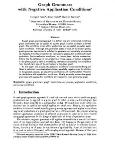
This section demonstrates that ELC grammars generate precisely the recursively enumerable graph languages. The proof uses a technique similar to an approach taken for “handle NLC” grammars in [12]. These are graph grammars which generate node-labeled graphs, but where the item replaced in a derivation step consists of an edge plus the edge’s source and target node. (These three things form a “handle”). The proof of the result begins with an ELC grammar scheme S, which can “simulate” graph programs. 5.1. Executing Graph Programs This section gives an ELC grammar scheme S, which “simulates” the graph programs of Section 4. The simulation occurs by starting with a graph which corresponds to some arbitrary graph program I,, Z,, .... Z,. From this starting point, the only terminal graph which S, can derive is the graph which the program Z, 7 Z,, ..*,Z, constructs. This is obtained by having the productions of S, execute the instructions of the graph program in a particular way. The terminal labels for S, are the labels of A. The non-terminals are the instructions (LEFT, RIGHT, EDGE., SWAP, ADD, IGNORE, SKIP, JOIN, END) plus five extra symbols (X, A, B, G, T). The connection relation is C x 2, where C is the set of all labels. The productions will be given after a short discussion. Suppose we have a graph program I,, I,, .... Z,, which encodes a graph ZL.When the graph program is executed, we can keep track of the graph as it is being constructed, and also we can keep track of the value of current at each step. Specilitally, let pi be the graph that exists after executing i instructions of the graph program (together with the information about how its nodes are numbered). Also, let current, be the value of current at this point. Thus, pLois the beginning graph, with two nodes (numbered 1 and 2) and no edges, while pL, is the final graph ,u. Now define some auxiliary graphs qO, q,, .... qn_ 2. The graph vi contains enough information to specify pi, the ordering on pL;s nodes, the value of current, and the list of remaining instructions (Z,+ i, ,.., I,). In particular, we define vi by adding some new nodes and edges to pi. The graph vi is shown in Fig. 5.1. The line of uncircled nodes at the bottom of the figure are the nodes of pi. They are connected in order by a sequence of X-edges, so that node number 1 is on the left and the highest numbered node is on the far right. The edges drawn below these nodes in the figure are the actual edges of pi. Above each node of pi is a “stick” of extra nodes. All but one of these sticks is a chain of two A-edges. The other stick is a chain of the remaining instructions Ii+, , .... Z,. The node number of the node which has the special “instruction stick” is also the value of current,. The explicit ELC grammar is constructed so that only one possible production
206
MAINANDROZENBERG
l A
A
A
A
x
...
...
> Edgesof pi
FIG. 5.1. The graph q,. The uncirclednodes are the nodes of p,.
can be applied to a graph like yli. This one production is completely determined by the next instruction in the “instruction stick.” For example, if the instruction Ii+ 1 is RIGHT, then there is a production which corresponds to the RIGHT instruction which can be applied to vi. The effect of applying this production is to move the instruction stick right one node. In this way, vi is transformed into vi+ 1. Finally, when qn_* is reached, there are only two instructions (END,END) remaining. At this point, some extra productions must be applied to Y]_~ to get rid of the extra nodes and edges. The final result will be the graph ,u,, = .LL Two more items should be mentioned about the qI graphs: Actually, it is possible to apply a “wrong” production to vi. For example, the LEFT production might be applied when it should be a RIGHT production. However, the application of a “wrong” production always results in one or more of the “sticks” becoming disconnected from the rest of the graph. Once this happens, the derivation can never finish with a terminal graph. In particular, the only way an A-edge or an END-edge can be removed is if there is a G or X edge in the same connected component of the graph. ??
The nodes which have attached “A-sticks” (i.e., those which are not currenti) may have a more complicated structure attached. This structure will be a graph of A and B edges. We require that this attached graph has at least one edge which is not connected to the uncircled node from pi, and that no B-edges are adjacent to this uncircled node. So, vi can actually be a bit more complicated than Figure 5.1. ??
Figures 5.2 through 5.12 show the productions which correspond to each of the instructions, together with an example of how these instructions would transform vi into vi+ i. As an example, we can look at the production for the RIGHTinstruction in detail (see Fig. 5.2). Prior to applying this production to an vi graph, the first instruction on the instruction stick of vi must be a RIGHTinstruction. After the production, we want the instruction stick to be “moved right one node,” and the RIGHT instruction to be removed. Actually, this is not quite the way the production works: after the production, the instruction stick has been “moved right one node,”
207
EDGE-LABEL CONROLLED GRAPH GRAMMARS
FIG. 5.2. Production Pl, the RIGHT instruction. Example derivation step: The edges C and D in this example are from the graph which is being constructed. The . . . indicates the instruction stick. The mother edge and daughter graph are indicated by dotted boxes.
x A I, /I
!
,
A
A
Ii
A
A
1 A 1
R
/I
LEFT
A
*
LEFr :. ,
C
A
I,
\ A
j
D
i__
R A
:
0
/\ x
D
, /
R
0
:
i\
/i I
IGNORE x
A j
A
__
C
FIG. 5.3. Production P2, the LEFT instruction. Example derivation step: The edges C and D in this example are from the graph which is being constructed. The t.. indicates the instruction stick. The mother edge and daughter graph are indicated by dotted boxes.
208
MAIN AND ROZENBERG
a
A A
A A
A
% A
%
x
%
Li----u i
Ii
A
A
EDGE
x j
....! x
A
mmy
1 I\
.. : :
A
I, i\
, Ii
A
X
D
C
D
;
Y
;
c
FIG. 5.4. Production P3 (for each YE .X), the EDGE ,,instruction. Example derivation step: The edges C and D in this example are from the graph which is being constructed. The indicates the instruction stick. The mother edge and daughter graph are indicated by dotted boxes.
but the RIGHT instruction is still on the stick. However, an IGNORE instruction has been inserted in front of the RIGHT instruction-which is the programmed equivalent of removing the RIGHT instruction. (In fact, this was the whole reason for including the IGNORE instruction in the instruction set.) An example of the RIGHT production in a derivation step is shown at the bottom of Fig. 5.2. Notice that the actual production is not applied to the RIGHT-edge itself, but rather to the X-edge whose source is also the source of the RIGHT-edge. Each of the other instructions is implemented similarly. The productions are given in the explicit ELC form. Recall that in the explicit form, each node u of a daughter graph has an explicit set L(U) of edge-labels which determines when it is an A-node. In the figures, we will write L(U) next to each node u of a daughter graph. S, denotes d u (X}; S, denotes A u {X, A}, and S3 denotes the set of instructions (LEFT, RIGHT, EDGE,, SWAP, ADD, IGNORE, SKIP, JOIN, END). We will use the notation from Section 2 to denote the Source and target subsets (0, 0, ? ? , @I ). The formal result that we need about this graph grammar Lemma 5.1.
scheme is stated in
LEMMA 5.1. Let P= II, .... Z, be a graph program which constructs some graph ~EEG~ (with 1~1> 1). Let vi (O< i 0). Actually, we can prove a result which is stronger than the lemma. The result is this: Let y be any
218
MAIN AND ROZENBERG
graphical form of G, and suppose the nodes of y are partitioned into m disjoint sets S, 7 S,, .*.,S,, where each set Si is connected. An unordered pair of sets {Si, Si} is called adjacent if there is an edge from a node of Si to a node of S,, or vice versa. We will prove that the total number of pairs of adjacent sets is no more than cm. (This immediately implies the lemma, by taking y to be a terminal graph and partitioning it into singleton nodes.) The proof of the stronge;result is an induction on the length of the derivation of y. The base step (y is -) is trivial. For the induction step, assume the result holds for graphical forms with derivations of length k, and suppose we now have a graphical form y with a derivation of length k + 1. Let S,, .... S, be the partition of y (as above). Also, let y’ be the next-to-last graphical form in the derivation of Y, and let X := (a, E,,,,,,, atarget) be the final production which takes y’ to y. (Recall that N,,,,,, and atargetmust be singleton sets. Because of this we will abuse notation and let %,urce and atarget be the actual single nodes rather than singleton sets of nodes.) The nodes of y’ are nearly identical to those of y. The only differences are that y’ has two extra nodes (the mother source and mother target) which y does not have, and y has the nodes of the daughter graph which y’ does not have. From this, we see that the partition S,, .... S, of y also gives us a partition S;, .... Sk of y’, as follows: If Lx,,“,,, is in set Sj, then the mother source node in y’ is in set S:; if utarge, is in set S;, then the mother target node in y’ is in set S:; each other node of y’ is placed in the same set as its corresponding node in y. Of course, some of the resulting partition sets of y’ may be empty, but this is not forbidden. We will let n denote the number of such empty sets in the partition of y’. Also note that if a node v of the daughter graph is in set Si, then Sl is either empty, or it contains the mother source or mother target. (Otherwise it is not connected.) What adjacent pairs can occur in the partition of y? There are only two sorts of adjacencies that can arise: 1. A pair {Si, S,} may be adjacent in y because {S:, S;} is adjacent in y’. By the induction hypothesis, the maximum number of such adjacencies is c(m - n). 2. Let Si be one of the sets which contains at least one of the daughter nodes, and let S, be a set such that S; is empty. These might be adjacent in y, even if they were not adjacent in y’ (since S, can contain one of the daughter graph nodes). Now, there are no more than c choices for Si and no more than n choices for Sj. Therefore, the number of adjacencies of this kind is no more than cn. Hence, the number of pairs of adjacent sets in y is no more than c(m - n) + cn = cm, as required. 1 One consequence of the above lemma is that the language G, of all graphs over by an ELC, grammar (when A is nonempty). However, when restriction 3 is removed, it is not difficult to generate G,, even if the other two restrictions are present. The technique is to first generate graphs with lots of edges, then selectively remove edges. This does not work when restriction 3 is
A cannot be generated
219
EDGE-LABELCONROLLEDGRAPHGRAMMARS
present, because graphs with “lots of edges” cannot be generated in the first place. This gives the following corollary: THEOREM
The lines indicated by solid arrows in the following diagram are
7.2.
proper inclusions: ELC
ProojI None of the classes on the lower right side of the diagram can generate the language G, of all graphs over A. But even ELC,, can easily generate this language. 1
8. REQUIRING A COMPLETE
CONNECTION
RELATION
ELC, grammars require the connection relation to be complete. This means that once an edge is established, it can never be removed, except by rewriting it or by “collapsing” its source and target nodes. We show three results about this restriction. First, we show that certain non-trivial language problems are decidable for ELC, grammars. This implies that the ELC, languages are a proper subclass of all R.E. languages. The other two results are combinatorial lemmas about the languages generated by ELC,, and ELC,, grammars. These lemmas are used to show three other proper inclusions of language classes. 8.1. The Reduction from R.E. For convenience, we assume throughout this subsection that all ELC grammars have nonterminal labels chosen from some fixed countably infinite set IV, and they have terminal labels chosen from some other fixed countably infinite set T. This does not effect the generative power of the grammars (up to a renaming of terminal labels). Suppose we have a collection of ELC grammars H. For example, H might be all of the ELC grammars, or perhaps only those grammars that meet certain specified
220
MAIN AND ROZENBERG
restrictions (like ELC,). The class of grammars H is called recursioe provided that it is decidable whether an arbitrary ELC-grammar is in H. A language problem on H is a problem of the form: “Gioen a grammar G (from H), does L(G)...?” The question (indicated by “...?‘) can be any yes-no question like “contain a discrete graph?’ or “contain an infinite number of graphs ?” A language problem on H is nontrivial if there are grammars in H where the answer is “yes,” and there are other grammars in H for which the answer is “no.” A modification of the proof of Rice’s theorem [ 151 gives us the following result. LEMMA 8.1. Let H be a recursive collection of ELC grammars such that every recursively enumerable graph language is generated by some grammar of H. Then every non-trivial language problem on H is undecidable.
Let H,, H,, ... be some effective enumeration of those grammars in H Proof which have no terminal symbols. Also, let yi denote the discrete graph with i nodes and no edges. A diagonalization argument shows that
K= {YilYi4Hi) is not a language generated by a grammar of H, hence K is not recursively enumerable. Next, consider the membership problem for H: Given a grammar H of H and a graph y, determine whether y E L(H). If this problem is decidable, then the following would be an R.E. string language (program
I Y, $ f&l
(where program is the function from Section 4). But, this would imply that K (from the previous paragraph) is recursively enumerable, which we know is not true. Therefore, the membership problem for H is undecidable. Finally, suppose P is a nontrivial language problem on H and suppose there is an algorithm to decide P. We can proceed as in the proof of Rice’s theorem to use this algorithm to decide the membership problem for H. By this contradiction we conclude that P must be undecidable. [ Now, consider ELC,. This class of grammars is recursive, but the “one-node” problem is decidable in this class, as shown in this lemma: LEMMA
8.2. Let G E ELC,. Zt is decidable whether the one-node graph is in L(G).
Proof: First, we define the “destructive” labels of G to be the smallest set of labels such that:
1. If X := ? ?is a production 2.
Let X := /3 be a production
of G, then X is destructive. of G. (We do not care what the source and
target sets are.) Define fi’ to be the subgraph of /I obtained by keeping only destruc-
tive edges. If fi’ is connected, then X is destructive.
221
EDGE-LABEL CONROLLED GRAPH GRAMMARS
Such a smallest set exists since the set of all labels meets these two conditions, and whenever two sets of labels meet the conditions then so does their intersection. In fact, the smallest set of labels to meet these two conditions can be computed by starting with those labels that must be destructive by rule 1, then continue to add any new labels that are forced to be destructive by rule 2 until eventually no new iff A’ is destructive. Therefore, labels need to be added. We claim that X 5 E L(G) iff the start label is destructive, and this can be determined by computing the set of destructive labels. 1 ??
??
Because the one-node problem is non-trivial, the previous two lemmas imply that ELC, does not generate all of the R.E. languages: THEOREM
8.3.
L(ELC, ) is u proper subclass of L(ELC).
8.2. A Result about Restrictions 1 and 2’ This section demonstrates that the graphs generated by ELC,, grammars always contain a certain simple kind of subgraph. The result needs a few preliminary definitions: DEFINITION 8.1.
Let y be a graph and S a subset of nodes(y).
a. neighborhood(S) = {v E nodes(y) - S 1there exists some node in S which is directly connected to v by an edge of y}. b. S is a 2-simple set in y provided that neighborhood (S) can be expressed as a union neighborhood(S) = N, u NZ, and for each v E S, either (i)
v is directly connected to none of neighborhood
(S), or
(ii)
v is directly connected to all of N, and none of N, -N,,
(iii)
v is directly connected to all of N, and none of N, -N,.
or
LEMMA 8.4. Let L be an ELC,, language. Then there exists a constant c such that for any MEL (with Inodes(a)l > c), there exists u’E L such that:
(a)
Jnodes(a)( = [nodes(x
and
(b)
~1’has a 2-simple subset S with 3 < ISI 6 c.
Proof: Let G be an ELC,* grammar generating L, and let c be the maximum number of nodes in a daughter graph of a production of G. Consider a graph u EL (with [nodes(a)1 > c), and a derivation S %>cp jc y sSG o! of tl. The graph y in this derivation is the first point in the derivation such that Inodes(y)( = modes(c The daughter graphs used in the remainder of the derivation all have precisely two nodes-otherwise the number of nodes in the graphical form grows beyond Inodes(a)l, and because of restriction 2, it cannot shrink again. Thus, each produc3 The results of this section were developed with Mark Brissenden. It is related to a similar result about NLC-grammars [6].
222
MAIN AND ROZENBERG
tion in the derivation y s, a is the replacement of a mother edge by zero or more new edges. In general, c( is obtained from y by replacing each nonterminal edge by zero or more terminal edges. We now modify the derivation y 5, CIas follows: 1. For each nonterminal label X which appears in y, choose some arbitrary two node graph 6, such that X sG 6,. Such a graph must exist, otherwise the derivation y 5, CIwould not be possible without increasing the number of nodes. 2. Apply the derivation X SG 6, to each nonterminal label in y. Let tl’be the resulting terminal graph. The graph tl’ is in L and has the same number of nodes as y and c(. In fact, since a’ is obtained by making single-edge replacements to y, we may as well identify the nodes of a’ with the nodes of y. Let S be the set of nodes in CI’that were introduced in the daughter graph of the step /I aG y, and let cr be this daughter graph. We have 3 d ISI < c. Moreover, S is 2-simple, which is shown as follows: The division of the neighborhood of S is N, v N,, where N, contains those neighborhood nodes which were adjacent to resourcein y, and Nz contains those neighborhood nodes which were adjacent to ctarget in y. Now the nodes of S are precisely the nodes of G‘,and there are three cases for such a node: 1. A node which is in neither osourcenor c-rtarget.Such a node is not directly connected to any node in N, or N,, since it cannot be directly connected to any of the neighborhood of o in the graphical form y. 2. A node which is in (T,,,,, but not otarget. Because of the complete connection relation, such a node must remain connected to all of N,. However, it cannot be directly connected to any of N, -N,, because it is not connected to any of these nodes in y. 3. A node which is in ctarget but not asource. Because of the complete connection relation, such a node must remain connected to all of N,. However, it cannot be directly connected to any of N, - N, , because it is not connected to any of these nodes in y. 1 If the connection relation is not complete, then it is possible to generate an infinite language of discrete graphs which does not meet the requirements of Lemma 8.4. In particular, the “wheel” graphs generated by Example 2.6 do not meet the requirement of the lemma. This is because the only 2-simple subgraphs of the n-node wheel graph have less that 3 nodes, or more than n - 3 nodes. Therefore, this language cannot be generated by an ELC,, grammar. However, Example 2.6 is an ELC, grammar, giving the result: THEOREM
8.5. L(ELC,,) is a proper subclass
8.3. A Result about Restrictions
of L(ELC,).
1 and 3
The primary result of this section is similar to the “interchange lemma” for context-free string languages [ 143. The result applies to ELC,3 grammars.
EDGE-LABEL CONROLLED
223
GRAPHGRAMMARS
LEMMA 8.6. Let L be an infinite language of discrete graphs, generated by an ELC,3 grammar. Then L contains four graphs a,, az, b,, pz such that a1 #/?, and
Inodes
- Inodes
= Inodes(j?i)1 - lnodes(jz)l.
The current version of the proof needs a number of preliminaries, some of which might be eliminated in a simplier proof. The rest of this section gives those preliminaries (which are not used elsewhere) and the proof. If we have a derivation step S: a * /II,in an ELC, gramThe follow function. mar, then the nodes of a can be mapped to the nodes of /? by a function follow,: nodes(a) + nodes(B). The function follow, maps the mother source node to the source node of the daughter graph, and it maps the mother target node to the target node of the daughter graph. All other nodes of a are also nodes of B, so follow, is the identity function on these nodes. Similarly, if D: a % /? is a derivation of zero or more steps, then we can define follow,: nodes(a) + nodes(B), by composing the follow functions of the individual derivation steps. A double-pointed graph (or DP-graph) is a triple (0 vi, v,), where 0 is a graph and vi, v2 are distinguished nodes of 0. A DP-graph is proper if its two distinguished nodes are not the same node. For a label X, we will abuse notation, and let X also stand for the proper two-node DP-graph with a single X-edge from the first node to the second node. We also ambiguously let denote the one-node DP-graph. We will use capital Greek (0, Y) for DP-graphs, and DISCRETE denotes the set of all discrete DP-graphs. DP-graphs.
??
The 0
operation on DP-graphs.
Let 0 = (0, v, , v2) and Y = (II/, wl, w2) be two DP-graphs. The graph 0 0 Y is obtained by “merging” 8 and $, and identifying their pairs of distinguished nodes. Here is an example:
We give the formal definition for the case where Y is proper or neither of the DP-graphs is proper. (The remaining case, where 0 is proper and Y is not proper, is symmetric to the case where Y is proper and 0 is not). In this case, the nodes of 00 Y are (nodes(O) u nodes(@)) - {wi, wZ}. The edges of 8 remain the same, as do those edges of tj which were not incident to its distinguished nodes. An edge whose source was wk (k = 1 or k = 2) in $ has a new source vk, and similarly for targets. (The exception is an edge between the two distinguished nodes of +, when 0 is not proper. Such an edge disappears, since we do not allow self-loops.) The 0 operafion on sets of DP-graphs. Let A and B be two sets of DPgraphs. The graph language A @B is defined as {0 0 Y 10 E A and YE B}.
224
MAINANDROZENBERG
LIT L,, L,. Let G be an ELC, grammar, and let 0 = (0, vl, v2) be a proper DP-graph. We can define three graph languages. The first language consists of the discrete graphs that can be generated from 0 without “collapsing” v1 and vl. The second language is the same, except v1 and v2 must be collapsed. The third language is needed for some special cases later on. L,(o)=
{(~,fOllOW,(V,),fOllOW,(V,))EDISCRETE( for some derivation D: 8 %- I,+,follow,(v,)
#followr,(v,))
OWD(V,),fOllOW,(V,)) E DISCRETE 1 LA@) = {W, f0 11 for some derivation D: 6 5 t+b,follow,(v,)
= follow,(v,)}
L3(0) = { YE DISCRETE 1for some derivation D: 8 5 $,
follow,(v,)
#follow,(v,),
(~5,follow,(v,),
follow,(v,))
Y is obtained from by merging the two points}.
In the last line, Y is obtained by identifying follow,(v,)
with follow,(v,).
Derivations of discrete graphs, Let G be an ELC,, grammar which generates only discrete graphs, and let (0 0 !Y) be a graphical form for G. The discrete graphs which can be generated from (0 + Y) are completely defined by
Now we can proceed. Proof of Lemma 8.6. Assume that L does not contain four graphs as specified in the lemma. From this, we will show that L contains only a finite number of graphs. Let G be the ELC,3 grammar which generates L. The proof proceeds by assigning a “type” to each derivation in G. There will be only a finite number of derivation types, and each derivation type will generate only a finite number of different graphs. Therefore, G generates only a finite number of graphs. Let S be the start symbol of the grammar, and consider a derivation D: S 5. y. We assign a “type” to this derivation as follows:
1. If L,(S) = (y}, then D has type “1”. Otherwise, continue to step 2. 2.
If L2(S) = (y}, then D has type “2”. Otherwise, continue to step 3.
3. If neither of the previous two steps has assigned a type to D, then there must be some label X, a proper DP-graph 0 and a pair (i, j) such that: A.
The derivation D has the form S %(X0
B.
(i, j) is (1, l), (2, 3), or (3, 2).
c.
IL,(X)l > 1.
D.
y E (L,(X) 0 L,(O)).
0) % y.
EDGE-LABELCONROLLED
225
GRAPHGRAMMARS
For example, we can choose X= S, and let 0 be the two-node discrete proper DP-graph, and conditions A-D will all be met for some (i, j). (In particular, condition C is met, because the derivation is not of type 1 or 2). The graphical form (X0 8) in condition A is called an undetermined point in the derivation, because the final graph in the derivation has not yet been determined. There may be many values of X, (i, j), and 0 which meet conditions A-D. We want to choose the values so that the undetermined point (X0 0) is as far right as possible. If there are several choices which are equally far right, then the decision between the choices is arbitrary. Given this choice, the type of the derivation D is “(X, i, j).” Clearly there are only a finite number of types of derivations. There is at most one graph generated by derivations of type 1, and at most one graph generated by derivations of type 2. It remains to show that for any type (X, i, j), there are only a finite number of different graphs generated by derivations of this type. The proof has three cases, depending on the value of (i, j). First, consider a type (X, 1, 1). The set L,(X) contains at least two discrete DP-graphs (from condition C). Let m, and m, be the sizes of two different discrete DP-graphs in L,(X). There must be some fixed integer n,, which depends only on X, such that whenever (X00) is a graphical form in G, then L,(O) contains at most one discrete DP-graph, and this DP-graph has the fixed number of nodes n,. (If there were two such sizes, say n, and n2, then G would generate four discrete graphs of sizes m, + n, -2,m,+n,-2,m,+n,-2andm,+n,-2.But,wehave already assumed that four such graphs do not exist.) Consider a derivation S f (_&‘@@)a (Y@O) 9 y of type (X, 1, l), where (X00) is the rightmost undetermined point of the derivation. Note that L,(Y) contains only one graph-otherwise (X0 0) would not be the rightmost undetermined point of the derivation. Let n, be the number of nodes in this one graph. This implies that the final graph y has exactly n, + n, - 2 nodes. Since there are only a finite number of choices for Y (because there are a finite number of production rules), this implies that there are only a finite number of different graphs that can be derived by a derivation of type (X, 1, 1). The cases of (X, 2, 3) and (X, 3,2) derivations are treated similarly. m If the connection relation is not complete, then it is possible to generate an infinite language of discrete graphs which does not have four graphs as specified in Lemma 8.6. In particular, the sizes of the discrete graphs generated by Example 2.7 are increasing exponentially. Therefore, this language does not meet the property of Lemma 8.6, and it cannot be generated by an ELC,3 grammar. However, Example 2.7 is an ELC,, grammar, giving the result: THEOREM
8.7. L(ELC,,)
proper subclass of L(ELC,,).
is a proper subclass of
L(ELC,),
and L(ELC,,J)
is a
226
MAINANDROZENBERG 9. DISCUSSION
We have introduced and studied a new graph grammar model (ELC grammars), with motivation from the previously studied node-label controlled (NLC) graph grammars and the edge-rewriting systems of Habel and Kreowski. The replacement procedure of ELC is completely controlled by edge-labels, in analogy to the NLC grammars where replacement is node-label controlled. Three simple restrictions placed on the ELC model results in the edge-rewriting systems of Habel and Kreowski. The ELC model has the complete power of recursive enumerability. In order to understand where this power arises, we have studied several obvious restrictions on the model, resulting in the following hierarchy diagram: ELC ,_,,,,,..,,....../.“”
1
\
_...” ,,..” ELC2 “.’ 1
kELC1
x.EL[
ELc12”------,I’p‘
,.,,,,,,,,,.,.,,,,.,,.....,......../.FLc13
ELC123
The solid arrows indicate proper inclusions of language classes, as shown in Sections 7 and 8. The remaining four dotted lines all correspond to removing restriction 2 (disjoint source and target sets). In one sense, we know that these four dotted lines are also proper inclusions, because it is impossible to generate the onenode graph in ELC,. (This is similar to the fact that context-sensitive string grammars cannot generate the empty string without an erasing rule.) However, apart from this special case, we do not currently know whether restriction 2 causes a reduction in power. In particular, if L is an ELC-language, is L - { } always an ELC,-language? (and similarly for the other three dotted lines). The fact that ELC grammars have the full power of recursive enumerability needs to be taken as a warning. In particular, Rice’s theorem implies that every non-trivial question about ELC-languages is undecidable. Hence, in most practical cases, where there is interest in parsing or other questions about the graphs being generated, we will need to work with models that are less powerful than ELC. In our current work we are considering the above three restrictions in this light, as well as the special case where source and target subsets are required to be the entire daughter graph. Here are several other natural research directions that we are continuing to study: ??
EDGE-LABEL CONROLLED GRAPH GRAMMARS
227
1. Research on the combinatorial properties and decidability properties of the individual subclasses of ELC grammars in our diagram. 2. Hopefully the results of the previous questions will help us to single out a central subclass of ELC grammars. Once such a central subclass arises, we would like to study this in more depth. A similar plan was followed for node-label control grammars, yielding the tractable subclass of boundary NLC grammars [16]. 3. We plan to undertake a comparison of ELC grammars with other wellknown classes of graph grammars. In particular, a careful comparison between ELC and NLC grammars (also on various sublevels) seems natural, since in both grammar models the replacement mechanism is driven by labels. This should contribute to our understanding of the subtle issue of node-edge duality in the context of graph replacement. Our preliminary research indicates that this is a complex issue which may lead to a consideration of hypergraph grammars. 4. There are also a number of technical issues concerning our model. For example, we do not currently allow loops in graphs, although loops are allowed in Habel-Kreowski’s edge-replacement systems. Is this a critical difference, or can loops be accommodated in the ELC model?
ACKNOWLEDGMENTS We thank the referees who provided suggestions that were particularly helpful in Sections 4.2 and 8.3. Mark Brissenden made suggestions for Section 8.2, and Hans-Jorg Kreowski simplified Section 5.2.
REFERENCES 1. B. COURCELLE, An axiomatic definition of context-free rewriting and it’s applications to NLC grammars, Theoret. Compur. Sci. 55 (1987), 141-181. 2. H. EHRIG, M. PFENDER,AND H. J. SCHNEIDER,Graph grammars-An algebraic approach, in “Proceedings, Conf. Switch. Automata Theory, 1973,” pp. 167-180. 3. A. HABELAND H.-J. KREOWSKI,On context-free graph languages generated by edge replacement, in “Graph-Grammars and Their Application to Computer Science, 2nd International Workshop” (H. Ehrig, M. Nagl, and G. Rozenberg, Eds.), Lecture Notes in Computer Science, Vol. 153, pp. 143-158, Springer-Verlag, Berlin, 1983. 4. A. HABELAND H.-J. KREOWSKI,“Characteristics of Graph Langages Generated by Edge Replacement,” Technical Report, Department of Computer Science, University of Bremen, 1985. 5. M. HARRISON,“Introduction to Formal Language Theory,” Addison-Wesley, Reading, MA, 1978. 6. J. HOFFMANN AND M. G. MAIN, “Results on NLC Grammars with One-letter Terminal Alphabets,” University of Colorado Technical Report Cu-CS-348-86, September 1986. 7. D. JANSSENS AND G. ROZENBERG, On the structure of node-label controlled graph languages, Inform. Sci. 20 (1980), 191-216. 8. D. JANSSENS AND G. ROZENBERG, Restrictions, extensions and variations of NLC grammars, Inform. Sci. 20 (1980), 217-244. 9. D. JANSSENSAND G. ROZENBERG,Decision problems for node-label controlled graph grammars, .I. Comput. System Sci. 22 (1981) 144177.
57114012-S
228
MAIN AND ROZENBERG
10. D. JAN~SENS AND G. ROZENBERG, Graph
grammars
with
neighbourhood
Theoret. Comput. Sci. 21 (1982), 55-74. 11. H. C. M. KLEIJN, M. F’ENTTONEN,G. ROZENBERG, AND K. SALOMAA,Direction Znform. and Control 63 (1984), 113-l 17. sensitive grammars,
controlled
embedding,
independent
context-
12. M. G. MAIN AND G. ROZENBERG, “Handle NLC Grammars and Languages,” University of Colorado Technical Report CU-CS-315-85 (1985), submitted for publication. 13. M. NAGL, A tutorial and bibliographical survey on graph grammars, in “Graph-Grammars and Their Application to Computer Science and Biology” (V. Claus, H. Ehrig, and G. Rozenberg, Eds.),
Lecture Notes in Computer Science, Vol. 73, pp. 70-126, Springer-Verlag, Berlin, 1978. 14. W. OGDEN, R. J. Ross, AND K. WINKLMANN, An “Interchange Lemma” for context-free languages, SIAM J. Comput. 14 (1985), 41&415. 15. H. G. RICE, Classes of recursively enumerable sets and their decision problems, Trans. Amer. Math. Sot. 89 (1953), 25-59. delinitions, normal forms, 16. G. ROZENBERG AND E. WELZL, Boundary NLC graph grammars-Basic and complexity, Inform. and Control 69 (1986), 136-167.