Self-tuning PI TCP flow controller for AQM routers ... - Semantic Scholar

Self-Tuning PI TCP Flow Controller for AQM Routers With Interval Gain and Phase Margin Assignment Yang Hong and Oliver W.W. Yang SITE, University of Ottawa Ottawa, Ontario K1N 6N5, Canada

Changcheng Huang Dept. of Systems and Computer Engineering Carleton University, Ottawa, ON K1S 5B6, Canada E-mail: [email protected]

E-mail: {yhong, yang}@site.uottawa.ca

Internet, which may result in slow response and cause possible buffer overflow. Self-tuning AQM controllers were presented in [8, 9], but these AQM controllers always self-tune even on slight traffic load changes.

Abstract- We propose a self-tuning proportional-integral (PI) controller for Active Queue Management (AQM) in the Internet. Classical control theory is applied in the controller design. We assign proper interval of gain and phase margins to achieve good AQM performance while adapting the AQM control system to great traffic load changes very well. Based on the knowledge of the queue size, our PI controller can regulate the TCP source window size to clamp the steady value of queue size to specified target buffer occupancy. OPNET simulations demonstrate that with our self-tuning PI controller applied, the network shows good stability robustness.

In this paper, we apply classical control theory in a selftuning PI controller design based on gain and phase margins. Instead of specifying a fixed value of the gain margin and phase margin, we assign intervals of gain and phase margins for AQM control system to real-time monitored so that selftuning PI controller can self-tune only when the load changes in the Internet drift the gain margin or phase margin outside the interval. Otherwise, self-tuning PI controller remains unchanged.

Keywords: Active Queue Management, PI Control, Gain Margin, Phase Margin, Self-Tune

1. INTRODUCTION Congestion control has become a critical problem in the development of the Internet. This is because congestion in the Internet can cause high packet loss rates, increased delays, and can even break the whole system by causing congestion collapse. TCP (Transmission Control Protocol) congestion control mechanism has been the basis of the operation of the Internet. It adopts the end-to-end window-based flow control to avoid congestion [1].

2. NETWORK MODELING The non-linear dynamic model for TCP/AQM was developed by [10] and has been linearized in [11]. Figure 1 depicts the linearized model considered in this paper.

-

The Internet mainly depends on the cooperative nature of TCP congestion control in order to limit packet loss and to fairly share network resources. Active Queue Management (AQM) is proposed for congestion avoidance by dropping packets when congestion is anticipated instead of waiting for the queue to become full. As the only AQM algorithm widely implemented in current industry, Random Early Detection (RED)[2] attempts to drop packets with a certain probability that is a function of the average queue size, when the incipient congestion is detected. However, it is very difficult to tune RED parameters in order to perform well under different traffic conditions. BLUE [3] is a self-configuring (adaptive) AQM mechanism, which uses packet loss and link underutilization events to adjust the rate of congestion notification. Random Exponential Marking (REM) [4] attempts to stabilize both the input rate around link capacity and the queue around a small target, regardless of the number of users sharing the link. It is typical to measure the stability robustness of the control system in the frequency domain using gain and phase margins [5]. Based on these margins, a PI controller was designed for industrial control system in [6]. Another PI controller has been proposed for TCP/AQM routers and yielded a unique solution in [7]. But it does not allow any flexibility to adjust the great variations in the load level of the IEEE Communications Society Globecom 2004

δp

C (s)

δq

P ( s)e − sR 0

G (s ) Figure 1. Block diagram of a linearized AQM control system

In the model C (s ) is the AQM controller, and P( s )e − sR0 is the “plant” of AQM control system. The transfer function P(s ) is the product of Ptcp (s) and Pqueue (s ) , where

N R0

R0C 2 2

2N and Pqueue ( s ) = (1) 2N 1 s+ 2 s+ R0 C R0 with R0 is Round-trip time, C is Link capacity (packets/sec) and N is Load factor (number of active long-lived TCP sessions) at the operating point. The link capacity C can be estimated by keeping track of the outgoing packets, while the round-trip time R0 can be estimated by the TCP throughput Ptcp ( s ) =

equation R0 = 2 N /(C p 0 ) , where p 0 is equilibrium packet drop probability (the output of AQM controller), as proposed in [8]. The number of active TCP sources N can be estimated by the method presented in [12].

1324

0-7803-8794-5/04/$20.00 © 2004 IEEE

Authorized licensed use limited to: Carleton University. Downloaded on October 6, 2008 at 15:4 from IEEE Xplore. Restrictions apply.

The open-loop transfer function of the linearized AQM control system can be described as G ( s) = P( s)C ( s )e − sR0 , where C ( s ) = K P + K I / s is the PI controller for AQM. Figure 2 shows the Nyquist diagram of G(s) [13]. Its gain margin Am is defined at the phase crossover frequency ω p , i.e. where ∠G ( jω p ) = −180 D when G ( jω g ) = 1 / Am , while its phase margin

φm

is defined at the gain crossover

frequency ω g , i.e. where ∠G ( jω g ) = −180 D + φ m when G ( jω g ) = 1 . Gain margin of more than 1 ( Am > 1 ) and

positive phase margin positive ( φ m > 0 ) can guarantee the stability of AQM control system in according with Nyquist Stability theorem [13].

 K  q ( jω g )  K P − j I  = −e jφm  ω g   where q ( s ) = P( s )e − sR0 control system.

(4)

 e jφ m    1 K I = ω p Im   = ω g Im  q( jω g )   Am q( jω p ) 

(5)

 −1    1 π f P (ω ) = Re   + jω Im   − < ∠q ( jω ) < −π A q ( j ω ) A q ( j ω ) 2 m m    

1

(6)

 − e jφ m   e jφ m  π f I (ω ) = Re   + jω Im  − + φ m < ∠q ( jω ) < −π + φ m ( ) ( ) 2 q j q j ω ω    

φm

G( jω g )

Figure 2. Nyquist Diagram of linearized AQM control system G(s)

3. THE SELF-TUNING PI CONTROLLER

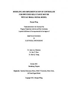
We can design self-tuning controller based on gain and phase margins of AQM control system. Our starting point is the transfer function of PI controller given by C ( s ) = K P + K I / s , where KP is the proportional gain and KI is integral gain. It is a common practice in the modern control that we normally specify the gain margin Am in the interval of 2≤Am≤4 and the phase margin φm in the interval of 300≤φm≤600 for good response, because too small a gain margin or phase margin will make the system sensitive to large load changes and cause instability, while too large a gain margin or phase margin will result in sluggish response to load changes. We adopt the method proposed by [6] to obtain the parameters of PI controller. So from the definition of the gain margin and phase margin [13], we can obtain

IEEE Communications Society Globecom 2004

   − e jφ m  −1 K P = Re   = Re    Am q ( jω p )   q ( jω g ) 

Since the frequency points ωp and ωg are unknown, we define the following two complex functions:

G( jω p )

 K  1 q( jω p )  K P − j I  = − ω A p  m  

represents the “plant” of AQM

It is noted that there are four unknowns altogether, namely, KP, KI, ωp, ωg in Equation (2) and (3). Observing that both equations are complex, they can be broken down to four real equations. Since the number of unknowns equals the number of real equations, we can obtain a unique solution. Splitting Equation (2) and (3) into their respective real and imaginary parts yields

1 Am

-1

(3)

(7) The functions fP(ω) and fI(ω) are plotted in the same complex plane. An intersection of these two functions means that they have the same real and imaginary parts, and thus both equation (4) and (5) are satisfied so that the intersection is a solution to equations (2) and (3) that provides a set of values for KP and KI, and the corresponding ωp and ωg, and no solution exists if they do not intersect. The solution will exist if we choose the proper phase margin and gain margin with the range of 2≤Am≤4 and 300≤φm≤600. When the parameters N, C and R0 of the network changed so greatly that the system gain margin or phase margin fell outside the specified interval, the self-tuning PI controller need to self-tune to give new Am and φm. This is done by realtime monitoring the gain and phase margins of the AQM control system using the following Equations (8), (9), (10) and (11), which we obtain according to the definition of gain margin and phase margin [13].   ωp − arctan 2N  2  R0 C

     − arctan ω p   1    R0 

2 Nω p ω 2p + ( Am =

(2)

1325

   − ω R = − π − arctan  K Pω p    p 0  2  KI    2N 2 1 ) ω 2p + ( )2 R0

R02C

C 2 K P2ω 2p + K I2

(8)

(9)

0-7803-8794-5/04/$20.00 © 2004 IEEE

Authorized licensed use limited to: Carleton University. Downloaded on October 6, 2008 at 15:4 from IEEE Xplore. Restrictions apply.

 2N   2N   1  K 2C 4  K 2C 4 ω g6 +   ( ) 2  +  ( ) 2  ω g4 + ( ) 2 − P ω g2 − I =0 2   R 3C   R02C   R0   4N  4N 2     0

(10)    K Pω g  π  ωg φ m = + arctan   − arctan 2 N 2  KI   2 R C  0

      ωg arctan −   1     R0 

    − ω g R0  

(11)

where the smallest positive real root of the Equation (10) will be the default value of gain crossover frequency ω g to calculate the phase margin of the control system by Equation (11). It is not difficult to show that Equation (8) holds true only when 0 ≤ ω p R0 < π / 2 . Based on the approximation that

For further performance analysis and evaluation, we shall consider a network system with TCP-Reno sources that use the Fast-Retransmit and Fast-Recovery mechanisms. We use N=100 greedy ftp (long-lived TCP flow) sources and 20 http (short-lived TCP flow) sources in the beginning of the experiment. The average end-to-end propagation delay can be approximated as 0.09 second. Considering the queuing delay, the upper limit of round trip time (RTT) is set as R0=0.25 second. The link bandwidth is T3 (44,736,000bps), with the average packet size being 536 bytes. It means that the link capacity is C=44736000/536/8 = 10433 packets/second. -6

10

x 10

8

tan( x) ≈ x when 0 ≤ x ≤ π / 4 , we can simplify Equation (8) in 2 different cases:

6

Case (1) when ω p R0 ≤ π / 4 : by taking tangent function on the Equation (8), we can obtain

2

A

f

I

4

0

-2

 2K I ω 4p +   R0 K p 

 N  1  4 N   2 2 NK I (12) 1 +     R C  − R 2 1 + R C  ω p − R 4 CK = 0 0  0   0  0 P

-4

-6

Case (2) when π / 4 < ω p R0 < π / 2 : by taking tangent function on the Equation (8), we can obtain

-8 -2

4

6

8 fP

10

12

14

16

18 -6

x 10

The smallest positive real root of the Equation (12) or (13) will be the default value of phase crossover frequency ω p to calculate the gain margin of the control system by Equation (9). We first use Equation (12) to derive ω p . Then we can calculate the value of ω p R0 . If we find π / 4 < ω p R0 < π / 2 , then we recalculate ω p by Equation (13). This provides us a design procedure for the self-tuning PI controller as follows: Step 1: Estimate the network parameters N, R0 and C, then specify the interval of gain margin and phase margin, the nominal gain margin Am and the nominal phase margin φm respectively. Step 2: Obtain the proportional gain K P and integral gain K I using Equations (4), (5), (6) and (7). Step 3: Apply Equations (8), (9), (10) and (11) to monitor the gain and phase margins of the AQM control system online. If the gain margin or phase margin falls outside the specified interval, go to Step 2. Otherwise, self-tuning PI controller remains unchanged.

1326

10 |G(ωg)|

0

|G(ωp)|

-10

-20

0

0.5

1

1.5

2 Frequency (rad/s)

2.5

3

3.5

4

-100 Phase response in degree

(13)

Magnitude response in db

20

  π  2N 2 NK  π  2 NK I π  πK    1 −  − 1 −  I ω p − 4 I 1 +  = 0 − 2 −  2  4 4 4 4 R CK K R C R CK   0 P   0  P  0 P  

IEEE Communications Society Globecom 2004

2

Figure 3. The graph of f P and f I

 2N  K  π 1 − I ω 3p +  2 −   R02C   R K 4  0 p   π  2 N  π 2 NK I  1  πK  1   2 +  2 + 1 + − − 2 +  I ω 2p −  4  K P  4 R0   CK P  R0  4  R0 C 

ω 4p + 

1 − 2 R0

0

-120

∠G(ωg) -140 -160

∠G(ωp)

-180 -200

0

0.5

1

1.5

2 Frequency (rad/s)

2.5

3

3.5

4

Figure 4. Frequency Response for the AQM Control System with Self-tuning PI Controller

Example: Using the network system described above, we shall choose the nominal gain margin Am as 3 (the mean of 2 and 4), and the nominal phase margin φm as 45° (the mean of 30° and 60°), so that the self-tuning PI controller can clamp the gain margin of control system inside the interval of 2 ≤ Am ≤ 4 , and the phase margin of control system inside the interval of 30 D ≤ φ m ≤ 60 D upon the great load changes. Then based on the Equations (2) to (7), we can draw a plot, as

0-7803-8794-5/04/$20.00 © 2004 IEEE

Authorized licensed use limited to: Carleton University. Downloaded on October 6, 2008 at 15:4 from IEEE Xplore. Restrictions apply.

4. PERFORMANCE EVALUATION AND ANALYSIS

We verify the self-tuning PI controller via simulations using OPNET Modeler based on the network topology shown in Figure 5. For the simplicity, we only draw 5 subnets with 5 respective links, while each subnet contains 20% of the total TCP sources respectively. We simulated the case of http and greedy ftp connections, i.e. the ftp sources always have data to send as long as their congestion windows allow. The receiver’s advertised window size is set sufficiently large so that TCP connections are not constrained at the destination. The buffer size is 1000 packets. The target buffer occupancy is specified as 400 packets. The notation AM means gain margin, and PM means phase margin. TCP Sources

TCP Destinations

30ms 40ms

10ms 20ms Router

1

Bottleneck Link

30ms

50ms

Router

Queue Size (Packets)

10ms 20ms

30ms 40ms

2

50ms

Figure 5. Network Topology for Simulation

1000 RED

800 600 400 200 0 1000

0

Figure 6 shows the instantaneous queue size of RED, fixed PI controller and our self-tuning PI controller upon the great traffic change. We also set the nominal gain margin as 3 (half way between 2 and 4) and the nominal phase margin as 45° (half way between 30° and 60°) in order to give room for our controller to self-tune. At time t=0, N=100 greedy ftp sources and 20 http sources were used, it was obvious that our self-

1327

40

80

120

160

200

800 600 400 200

PI Controller

0 1000

0

40

80

120

160

200

Self-Tuning PI Controller

800 600 400 200 0 0

We have run the RED algorithm [2] and the fixed PI controller in [7] for comparison. We use the similar RED parameters as in [7]. That is, maximum value for drop probability pmax is 0.1; the maximum queue threshold maxth is 700; the minimum queue threshold minth is 150; the queue weight wq is 1.33×10-6. In all the graphs shown subsequently in the paper, we depict the time evolution of the instantaneous queue size, with the time axis drawn in seconds.

IEEE Communications Society Globecom 2004

Queue Size (Packets)

Figure 4 is the Bode plot in the range of 0.1 ≤ ω ≤ 4 for the control system. Both the magnitude |G(s)| and phase ∠G(s) are decreasing function of ω as expected. It is shown that the nominal gain margin and phase margin of AQM control system with the self-tuning PI Controller have been pegged at Am=3 and φm= 45° as desired.

tuning PI controller showed a better response than RED. Its settling time was much shorter than RED. Also the response time of our self-tuning PI controller was shorter than the fixed PI controller. Furthermore our method showed less oscillation. At time t=100sec, 300 greedy ftp sources and 60 http sources were added. The instantaneous queue size of both RED and fixed PI controller exhibited sluggish response. The instantaneous queue size of fixed PI controller increased to more than 800 packets and some buffer overflow occurred between t=100 sec and t=140 sec. Both the gain margin and the phase margin of self-tuning PI control system had gone beyond their specified intervals, so our self-tuning PI controller self-tuned and gave new Am=3 and φm=45°. It can be seen that the instantaneous queue size of our self-tuning PI controller still reached around the target buffer occupancy (400 packets) very quickly.

Queue Size (Packets)

shown in Figure 3. From the Figure 3 (Point A), we can obtain 4.84 × 10 −6 PI Controller as C ( s ) = 1.054 × 10 −5 + . Next, we s apply the Equations (8) to (11) to real-time monitor the gain and phase margin of AQM control system. If the gain margin or phase margin falls outside the interval, PI controller will self-tune based on Equations (2) to (7).

40

80

120

160

200

Time (Seconds) Figure 6. Instantaneous Queue Size Comparison of RED, Fixed PI controller [7] and our Self-tuning PI Controller

Figure 7 shows the instantaneous queue size of self-tuning AQM controller in [8] and our self-tuning PI controller upon the small traffic change. At the time t=0sec, N=100 greedy ftp sources and 20 http sources were used. The response time of self-tuning PI controller was shorter than the self-tuning AQM controller. At time t=100sec, N=70 greedy ftp sources and 20 http sources were used. Due to the change of the network environment, self-tuning AQM controller always self-tuned and gave the new PI controller. It can be seen that the queue size decreased till the buffer was nearly empty and then increased and approached the target buffer occupancy (400 packets). Both the gain margin and the phase margin did not

0-7803-8794-5/04/$20.00 © 2004 IEEE

Authorized licensed use limited to: Carleton University. Downloaded on October 6, 2008 at 15:4 from IEEE Xplore. Restrictions apply.

Queue Size (Packets)

Queue Size (Packets)

drift outside the specified interval respectively, the self-tuning PI controller remained unchanged. However, the queue size had little fluctuation upon this slight traffic change. At the time t=200sec, N=130 greedy ftp sources and 30 http sources were used. Self-tuning AQM controller also self-tuned and got the new PI controller. The queue size had more oscillation than that of self-tuning PI controller before it reached the target buffer occupancy and also had a small spike. Both the gain margin and the phase margin still did not drift outside the specified interval respectively, the self-tuning PI controller remained unchanged. However, the queue size had little fluctuation except one small spike. 1000

We want to appreciate the financial support from NSERC Postgraduate Scholarship (PGS-B) and NSERC Research Grant (#OGP0042878). REFERENCES

[1] S. Floyd and K. Fall, “Promoting the Use of End-to-End [2] [3]

Self-Tuning AQM

800

ACKNOWLEDGMENT

600

[4]

400 200

[5]

0 1000

0

60

120

180

240

300

[6]

Self-Tuning PI Controller

800 600

[7]

400 200 0

[8] 0

60

120

180

240

300

Time (Seconds)

[9]

Figure 7. Instantaneous Queue Size Comparison of Self-Tuning AQM Controller [8] and our Self-Tuning PI Controller

5. CONCLUSION We have applied classical control theory to develop a selftuning PI controller for AQM routers in the Internet based on gain and phase margin specifications. Instead of a fixed value, we assign the proper intervals within which the self-tuning PI controller only self-tunes when the gain margin or phase margin of AQM control system goes outside the interval. Equations for designing the self-tuning PI controller as well as those for real-time monitoring of gain and phase margins of AQM control system are derived. Furthermore, based on the knowledge of the queue size, the PI controller can regulate the TCP source window size to clamp the steady value of queue size to the specified target buffer occupancy. The simulations demonstrate that our self-tuning PI controller can adapt AQM control system to the change of network environment very well and the network shows good stability robustness.

IEEE Communications Society Globecom 2004

1328

[10]

[11]

[12] [13]

Congestion Control in the Internet”, IEEE/ACM Transactions on Networking, Vol. 7, No. 4, August 1999, pp. 458-472. S. Floyd and V. Jacobson, “Random Early Detection Gateways for Congestion Avoidance”, IEEE/ACM Transactions on Networking, Vol. 1, No. 4, August 1993, pp. 397-413. W. Feng, D. Kandlur, D. Saha and K. Shin, “Blue: A New Class of Active Queue Management Algorithms”, In UM CSETR_387-99, April 1999. S. Athuraliya, V. H. Li, S. H. Low and Q. Yin, “REM: Active Queue Management”, IEEE Network, 15(3), May/June 2001, pp. 48-53. W.K. Ho, T.H. Lee, H.P. Han and Y. Hong “Self-Tuning IMCPID Control with Interval Gain and Phase Margin Assignment”, IEEE Transactions on Control Systems Technology, Vol. 9, No. 3, May 2001, pp. 535-541. Fung H.K., Q.G. Wang and T.H. Lee “PI Tuning in Terms of Gain and Phase Margins”, Automatica, Vol. 34, 9, September 1998, pp. 1145-1149. C.V. Hollot, Vishal Misra, Don Towsley, and Wei-Bo Gong, “On Designing Improved Controllers for AQM Routers Supporting TCP Flows,” in Proceedings of IEEE/INFOCOM, April 2001. Honggang Zhang, C.V. Hollot, Don Towsley and Vishal Misra, “A Self-Tuning Structure for Adaptation in TCP/AQM Networks”, in Proceedings of IEEE/Globecom 2003, pp. 1346 – 1355. Wei Wu, Yong Ren, Xiuming Shan, “A Self-Configuring PI Controller for Active Queue Management”, Proceedings of the 7th Asia-Pacific Communication Conference (APCC'2001), Tokyo Japan, Sep. 2001. Vishal Misra, Wei-Bo Gong, and Don Towsley, “Fluid-based Analysis of a Network of AQM Routers Supporting TCP Flows with an Application to RED,” in Proceedings of ACM/SIGCOMM, 2000. C.V. Hollot, Vishal Misra, Don Towsley, and Wei-Bo Gong, “A Control Theoretic Analysis of RED,” in Proceedings of IEEE/INFOCOM, April 2001. Ott, T.J., Lakshman, T.V., Wong, L.H., “SRED: stabilized RED,” in Proceedings of IEEE/INFOCOM 1999, pp. 1346 – 1355. Katsuhiko Ogata, Modern Control Engineering, 4th Edition, Prentice Hall, 2002.

0-7803-8794-5/04/$20.00 © 2004 IEEE

Authorized licensed use limited to: Carleton University. Downloaded on October 6, 2008 at 15:4 from IEEE Xplore. Restrictions apply.