Semantic Models for Machine Learning - CiteSeerX

UNIVERSITY OF SOUTHAMPTON

Semantic Models for Machine Learning

by David Roi Hardoon

A thesis submitted in partial fulfillment for the degree of Doctor of Philosophy

in the Faculty of Engineering, Science and Mathematics School of Electronics and Computer Science

February, 2006

UNIVERSITY OF SOUTHAMPTON ABSTRACT FACULTY OF ENGINEERING, SCIENCE AND MATHEMATICS SCHOOL OF ELECTRONICS AND COMPUTER SCIENCE Doctor of Philosophy by David Roi Hardoon

In this thesis we present approaches to the creation and usage of semantic models by the analysis of the data spread in the feature space. We aim to introduce the general notion of using feature selection techniques in machine learning applications. The applied approaches obtain new feature directions on data, such that machine learning applications would show an increase in performance. We review three principle methods that are used throughout the thesis. Firstly Canonical Correlation Analysis (CCA), which is a method of correlating linear relationships between two multidimensional variables. CCA can be seen as using complex labels as a way of guiding feature selection towards the underlying semantics. CCA makes use of two views of the same semantic object to extract a representation of the semantics. Secondly Partial Least Squares (PLS), a method similar to CCA. It selects feature directions that are useful for the task at hand, though PLS only uses one view of an object and the label as the corresponding pair. PLS could be thought of as a method that looks for directions that are good for distinguishing the different labels. The third method is the Fisher kernel. A method that aims to extract more information of a generative model than simply by their output probabilities. The aim is to analyse how the Fisher score depends on the model and which aspects of the model are important in determining the Fisher score. We focus our theoretical investigation primarily on CCA and its kernel variant. Providing a theoretical analysis of the method’s stability using Rademacher complexity, hence deriving the error bound for new data. We conclude the thesis by applying the described approaches to problems in the various fields of image, text, music application and medical analysis, describing several novel applications on relevant real-world data. The aim of the thesis is to provide a theoretical understanding of semantic models, while also providing a good application foundation on how these models can be practically used.

Contents Nomenclature

xiii

Acknowledgements

xv

1 Introduction 1.1 Learning . . . . . . . . . . . . . . . . . . . . . . . . . . . . . . . . . . . . . 1.2 The Usage of Features . . . . . . . . . . . . . . . . . . . . . . . . . . . . . 1.3 Thesis Contributions & Outline . . . . . . . . . . . . . . . . . . . . . . . .

1 1 2 2

I

5

Theory

2 Enabling Technologies 2.1 Kernel Methods . . . . . . . . . . . . . . . . . . . 2.1.1 Limitations of Linear Learning . . . . . . 2.1.2 Learning in Feature Space . . . . . . . . . 2.1.3 The Kernel Function . . . . . . . . . . . . 2.1.3.1 Properties of Kernels . . . . . . 2.2 Dual Partial Gram-Schmidt Orthonormalisation . 2.3 Eigen Analysis . . . . . . . . . . . . . . . . . . . 2.4 Support Vector Machines . . . . . . . . . . . . . 2.5 Summary . . . . . . . . . . . . . . . . . . . . . .

. . . . . . . . .

3 Semantic Models 3.1 Semantic Representation by Linear Regression . . 3.1.1 Partial Least Squares . . . . . . . . . . . . 3.1.2 Kernel Partial Least Squares . . . . . . . . 3.2 Introduction to Canonical Correlation Analysis . . 3.2.1 Example . . . . . . . . . . . . . . . . . . . . 3.3 Probabilistic Approach to Semantic Representation 3.4 Summary . . . . . . . . . . . . . . . . . . . . . . .

. . . . . . . . .

. . . . . . . . .

. . . . . . . . .

. . . . . . . . .

. . . . . . . . .

. . . . . . . . .

. . . . . . . . .

. . . . . . . . .

. . . . . . . . .

. . . . . . . . .

. . . . . . . . .

. . . . . . . . .

. . . . . . . . .

7 7 7 11 12 13 15 18 20 22

. . . . . . .

. . . . . . .

. . . . . . .

. . . . . . .

. . . . . . .

. . . . . . .

. . . . . . .

. . . . . . .

. . . . . . .

. . . . . . .

. . . . . . .

. . . . . . .

23 23 25 27 29 29 32 35

4 Canonical Correlation Analysis; A Detailed Review 4.1 Canonical Correlation Analysis . . . . . . . . . . . . . 4.2 Kernel Canonical Correlation Analysis . . . . . . . . . 4.3 Statistical Analysis of Canonical Correlation Analysis 4.3.1 k-dimensional Analysis . . . . . . . . . . . . . . 4.4 Regularised Kernel Canonical Correlation Analysis . .

. . . . .

. . . . .

. . . . .

. . . . .

. . . . .

. . . . .

. . . . .

. . . . .

. . . . .

. . . . .

. . . . .

37 37 40 42 44 44

v

. . . . . . .

vi

CONTENTS

4.5 4.6 4.7

II

4.4.1 Regularisation via Optimisation Function . . 4.4.2 Regularisation via Optimisation Constraint . Regularised Kernel CCA with Matrix Decomposition 4.5.1 Selecting Regularisation Parameter τ . . . . . Example on Toy Data . . . . . . . . . . . . . . . . . Summary . . . . . . . . . . . . . . . . . . . . . . . .

. . . . . .

. . . . . .

. . . . . .

. . . . . .

. . . . . .

. . . . . .

. . . . . .

. . . . . .

. . . . . .

. . . . . .

. . . . . .

. . . . . .

Application

5 Imagery & Text Taxonomy 5.1 Generic Object Recognition . . . . . . 5.1.1 Proposed System . . . . . . . . 5.1.2 Database Description & Setup 5.1.3 Performance & Conclusions . . 5.2 Generating Category-based Documents 5.2.1 Generating a New Document . 5.2.2 Problem Setup . . . . . . . . . 5.2.3 Generation Results . . . . . . . 5.2.4 Conclusions . . . . . . . . . . . 5.3 Summary . . . . . . . . . . . . . . . .

45 46 47 48 49 51

53

. . . . . . . . . .

. . . . . . . . . .

. . . . . . . . . .

. . . . . . . . . .

. . . . . . . . . .

. . . . . . . . . .

. . . . . . . . . .

. . . . . . . . . .

. . . . . . . . . .

. . . . . . . . . .

55 55 56 57 59 60 61 62 64 67 68

6 Music 6.1 Identifying Famous Performers From Their Playing Style . 6.1.1 Representing Music . . . . . . . . . . . . . . . . . 6.1.2 String Kernels . . . . . . . . . . . . . . . . . . . . 6.1.3 Experiments . . . . . . . . . . . . . . . . . . . . . 6.1.4 Conclusions . . . . . . . . . . . . . . . . . . . . . . 6.2 Identifying Famous Composers from Their Sheet Music . 6.2.1 Hidden Markov Model for Sheet Music . . . . . . . 6.2.2 Compositions Used & Setup . . . . . . . . . . . . . 6.2.3 Sheet Music Generation . . . . . . . . . . . . . . . 6.2.4 Identification . . . . . . . . . . . . . . . . . . . . . 6.2.5 Conclusions . . . . . . . . . . . . . . . . . . . . . . 6.3 Summary . . . . . . . . . . . . . . . . . . . . . . . . . . .

. . . . . . . . . . . .

. . . . . . . . . . . .

. . . . . . . . . . . .

. . . . . . . . . . . .

. . . . . . . . . . . .

. . . . . . . . . . . .

. . . . . . . . . . . .

. . . . . . . . . . . .

. . . . . . . . . . . .

71 71 72 74 75 78 78 79 82 83 84 86 87

7 Medical Analysis 7.1 Functional Magnetic Resonance Imaging 7.2 fMRI Activity Analysis . . . . . . . . . 7.2.1 Simulated Data . . . . . . . . . . 7.2.2 Finger Flexing . . . . . . . . . . 7.2.3 Mental Calculation . . . . . . . . 7.3 Signal Reconstruction . . . . . . . . . . 7.4 Classifying Cognitive States . . . . . . . 7.4.1 Applied Learning Techniques . . 7.4.2 Motor Tasks . . . . . . . . . . . 7.4.2.1 First Session . . . . . . 7.4.2.2 Second Session . . . . .

. . . . . . . . . . .

. . . . . . . . . . .

. . . . . . . . . . .

. . . . . . . . . . .

. . . . . . . . . . .

. . . . . . . . . . .

. . . . . . . . . . .

. . . . . . . . . . .

. . . . . . . . . . .

89 89 92 93 98 98 102 103 105 107 108 109

. . . . . . . . . .

. . . . . . . . . .

. . . . . . . . . . .

. . . . . . . . . .

. . . . . . . . . . .

. . . . . . . . . .

. . . . . . . . . . .

. . . . . . . . . .

. . . . . . . . . . .

. . . . . . . . . .

. . . . . . . . . . .

. . . . . . . . . .

. . . . . . . . . . .

. . . . . . . . . .

. . . . . . . . . . .

. . . . . . . . . .

. . . . . . . . . . .

. . . . . . . . . .

. . . . . . . . . . .

. . . . . . . . . . .

CONTENTS

7.5

vii

7.4.3 Visual Tasks . . . . . . . . . . . . . . . . . . . . . . . . . . . . . . 110 Summary . . . . . . . . . . . . . . . . . . . . . . . . . . . . . . . . . . . . 113

8 Conclusions 115 8.1 Open Discussion . . . . . . . . . . . . . . . . . . . . . . . . . . . . . . . . 115 8.2 Future Research . . . . . . . . . . . . . . . . . . . . . . . . . . . . . . . . 117

III

Back Matter

A Definitions A.1 Euclidean inner product . . . . A.2 Matrix Trace . . . . . . . . . . A.3 Empirical expectation . . . . . A.4 Karush-Kuhn-Tucker Condition A.5 Cholesky Decomposition . . . . A.6 Rademacher Complexity . . . .

119

. . . . . .

. . . . . .

. . . . . .

. . . . . .

. . . . . .

. . . . . .

. . . . . .

. . . . . .

. . . . . .

. . . . . .

. . . . . .

B Proofs & Derivations B.1 For Chapter 2 . . . . . . . . . . . . . . . . . . . . . B.1.1 SVM Optimisation . . . . . . . . . . . . . . B.1.2 SVM Optimisation with Penalty Parameter B.1.3 Gram-Schmidt Orthonormalisation . . . . . B.2 Proofs for Chapter 4 . . . . . . . . . . . . . . . . . B.2.1 Partial Derivatives of CCA . . . . . . . . . B.2.2 Feature Mapping and Weight Vector . . . . B.2.3 Norm of the Weight Vector . . . . . . . . . B.2.4 Kernel Function . . . . . . . . . . . . . . . B.2.5 k-dimensional Analysis . . . . . . . . . . . . B.2.6 CCA Link to PLS . . . . . . . . . . . . . . Bibliography

. . . . . .

. . . . . . . . . . .

. . . . . .

. . . . . . . . . . .

. . . . . .

. . . . . . . . . . .

. . . . . .

. . . . . . . . . . .

. . . . . .

. . . . . . . . . . .

. . . . . .

. . . . . . . . . . .

. . . . . .

. . . . . . . . . . .

. . . . . .

. . . . . . . . . . .

. . . . . .

. . . . . . . . . . .

. . . . . .

. . . . . . . . . . .

. . . . . .

. . . . . . . . . . .

. . . . . .

121 . 121 . 121 . 122 . 122 . 123 . 123

. . . . . . . . . . .

125 . 125 . 125 . 126 . 126 . 127 . 127 . 128 . 128 . 129 . 129 . 130 133

List of Figures 2.1 2.2 2.3 2.4 2.5 2.6

A separating hyperplane (w, b) for a two dimensional data set . . Maximising the distance between the two supporting hyperplanes Example of monotonic function . . . . . . . . . . . . . . . . . . . Data separable in feature space . . . . . . . . . . . . . . . . . . . Principle directions on a Gaussian. . . . . . . . . . . . . . . . . . Illustrating the Eigenprogram . . . . . . . . . . . . . . . . . . . .

3.1

Correlation Example . . . . . . . . . . . . . . . . . . . . . . . . . . . . . . 30

4.1 4.2

Affect of eigenvector and regularisation parameter selection on toy data. . 50 Affect of eigenvector and regularisation parameter selection on toy data (side and upper view). . . . . . . . . . . . . . . . . . . . . . . . . . . . . . 50 Affect of regularisation parameter selection on toy data for a selection of 91 eigenvectors. . . . . . . . . . . . . . . . . . . . . . . . . . . . . . . . . . 51

4.3

. . . . . .

. . . . . .

. . . . . .

. . . . . .

8 10 10 12 18 19

5.1 5.2 5.3 5.4 5.5 5.6 5.7 5.8

Proposed generic object recognition system Examples of dataset one . . . . . . . . . . . Categories of words in dictionary . . . . . . Document generation to Aviation image . . Document generation to Aviation image . . Document generation to Paintball image . . Document generation to Paintball image . . Document generation to Sports image . . .

. . . . . . . .

. . . . . . . .

. . . . . . . .

. . . . . . . .

. . . . . . . .

. . . . . . . .

. . . . . . . .

. . . . . . . .

. . . . . . . .

. . . . . . . .

. . . . . . . .

. . . . . . . .

. . . . . . . .

. . . . . . . .

. . . . . . . .

. . . . . . . .

58 58 63 67 67 68 68 69

6.1 6.2 6.3 6.4 6.5 6.6 6.7

The performance worm . . . . . . . . . . . . . Handling of a note of length 14 in the HMM . . Proposed scale invariant HMM for sheet music Mozart HMM generated sequence . . . . . . . . Bach HMM generated sequence . . . . . . . . . Beethoven HMM generated sequence . . . . . . Handel HMM generated sequence . . . . . . . .

. . . . . . .

. . . . . . .

. . . . . . .

. . . . . . .

. . . . . . .

. . . . . . .

. . . . . . .

. . . . . . .

. . . . . . .

. . . . . . .

. . . . . . .

. . . . . . .

. . . . . . .

. . . . . . .

. . . . . . .

73 80 80 83 83 84 84

7.1 7.2 7.3 7.4 7.5 7.6 7.7

Example of fMRI scans . . . . . . . . . . fMRI Time-seqeunce example . . . . . . . Square-wave reference time-sequence . . . Application of CCA to fMRI pixel region Embedded fMRI synthetic activity . . . . Simulated fMRI OCA correlation . . . . . Simulated fMRI CCA correlation . . . . .

. . . . . . .

. . . . . . .

. . . . . . .

. . . . . . .

. . . . . . .

. . . . . . .

. . . . . . .

. . . . . . .

. . . . . . .

. . . . . . .

. . . . . . .

. . . . . . .

. . . . . . .

. . . . . . .

. . . . . . .

90 91 91 93 94 94 95

ix

. . . . . . .

. . . . . . . .

. . . . . .

. . . . . . .

. . . . . . .

x

LIST OF FIGURES 7.8 7.9 7.10 7.11 7.12 7.13 7.14 7.15 7.16 7.17 7.18 7.19 7.20 7.21

Simulated fMRI KCCA weights . . . . . . . . . . . . . . . . Simulated fMRI OCA found true/false-positive . . . . . . . Simulated fMRI CCA found true/false-positive . . . . . . . Simulated fMRI KCCA found true/false-positive . . . . . . Recall vs. Precision for simulated fMRI. . . . . . . . . . . . Finger flexing fMRI OCA correlation . . . . . . . . . . . . . Finger flexing fMRI CCA correlation . . . . . . . . . . . . . Finger flexing fMRI KCCA weights . . . . . . . . . . . . . . Mental activity fMRI OCA correlation . . . . . . . . . . . . Mental activity fMRI CCA correlation . . . . . . . . . . . . Mental activity fMRI KCCA weights . . . . . . . . . . . . . Activity plot of the mental process prior to the motor one. . Bottleneck Neural Network architecture . . . . . . . . . . . Bottleneck Neural-Network training error . . . . . . . . . .

. . . . . . . . . . . . . .

. . . . . . . . . . . . . .

. . . . . . . . . . . . . .

. . . . . . . . . . . . . .

. . . . . . . . . . . . . .

. . . . . . . . . . . . . .

. . . . . . . . . . . . . .

. . . . . . . . . . . . . .

95 96 96 96 97 99 99 100 100 101 101 104 106 107

List of Tables 3.1 3.2

Computing correlation values using ordinary correlation . . . . . . . . . . 31 Computing correlation values using canonical correlation . . . . . . . . . . 32

5.1 5.2 5.3 5.4 5.5 5.6 5.7

Dataset one ROC Equal Error Rate comparison. Dataset two ROC Equal Error Rate comparison. Category words example . . . . . . . . . . . . . . KCCA: Success results using term frequency. . . GSVM: Success results using term frequency . . KCCA: Success results using TFIDF features. . . GSVM: Success results using TFIDF . . . . . . .

. . . . . . .

59 60 63 66 66 66 66

6.1 6.2 6.3 6.4 6.5 6.6 6.7 6.8

Movements of Mozart piano sonatas selected for analysis . . . . . . . . . . List of pianists and recordings used for style identification . . . . . . . . . Comparison of PLS with and without reweighting . . . . . . . . . . . . . . Performer identification from style, algorithms results comparison . . . . . Composer identification area under ROC using the HMM . . . . . . . . . Composer identification area under ROC using the Fisher linear kernel . . Composer identification area under ROC using the Fisher Gaussian kernel Composer identification area under ROC using the Fisher Gaussian kernel for combined HMMs . . . . . . . . . . . . . . . . . . . . . . . . . . . . . .

72 74 76 77 85 85 86

Reconstructing the test fMRI activity time sequence . . . . . . . . . . . . Bottleneck Neural-Network compression comparison . . . . . . . . . . . . First session motor fMRI SVM results . . . . . . . . . . . . . . . . . . . . First session motor fMRI method result comparison . . . . . . . . . . . . First session motor fMRI methods statistics - positive testing samples . . First session motor fMRI methods statistics - negative testing samples . . Second session motor fMRI method result comparison . . . . . . . . . . . Second session motor fMRI methods statistics - positive testing samples . Second session motor fMRI methods statistics - negative testing samples . Vision fMRI, SVM results on separate individuals . . . . . . . . . . . . . . Vision fMRI, SVM results on combined individuals . . . . . . . . . . . . . Vision fMRI, bottleneck Neural-Network results on combined individuals . Vision fMRI, one-class SVM results on combined individuals . . . . . . .

103 107 108 109 109 109 110 110 110 111 112 112 112

7.1 7.2 7.3 7.4 7.5 7.6 7.7 7.8 7.9 7.10 7.11 7.12 7.13

xi

. . . . . . .

. . . . . . .

. . . . . . .

. . . . . . .

. . . . . . .

. . . . . . .

. . . . . . .

. . . . . . .

. . . . . . .

. . . . . . .

. . . . . . .

. . . . . . .

. . . . . . .

86

Nomenclature w

The weight vector

b

The bias

x

Bold face letters denotes a vector

A0

Denotes a transpose of a matrix or vector A

E ˆ E

True expectation

I

The identity matrix

L

The Lagrangian

k·k

Is the 2-norm

k · kF ~ A

Is the Frobenious norm

`

Number of samples

φ(·)

Feature projection

F

The Feature space

h·, ·i

Inner product

κ(x, z)

The kernel function hφ(x), φ(z)i

K

The kernel matrix

δ

The Kronecker δij defined to be 1 if i = j else 0

trace(A)

The trace of matrix A

·◦·

Denotes the Frobenius inner product between matrices

ξ

The SVM slack variable

A−1

Denotes the inverse of A

j

The unit vector

Empirical expectation

Creates a row vector out of the entries of matrix A by concatenating its rows

xiii

Acknowledgements The process of obtaining a PhD degree is that of interaction and research. I would like to thank the many individuals named as well as unnamed, who have helped me throughout this process. Starting with my supervisors Prof. John Shawe-Taylor and Dr. Craig Saunders, who backed me from stage one, guiding and advising me through this labyrinthian process. Dr. Sandor Szdemak who never ceases to amaze me with his vast knowledge and infinite patience. Zakria “The Dawg” Hussain who has helped me keep my sanity throughout the many ordeals one can be subjected to during this long PhD process. I would like to thank the following individuals who I met during my first year at Royal Holloway, University of London; Dr. Chris Watkins, Dr. Jaz Kandola, Dr. Thore Graepel, Dr. Helen Threhane, Dr. Juho Rousu and Dr. Alexei Vinokourov. I would also like to thank the following individuals with whom I have had the pleasure of meeting during the remainder of my PhD studies and work in the Information: Signals, Images, Systems research group at the University of Southampton; Dr. Hongying Meng and Dr. Jason Farquhar. All who have provided me with means of expanding my understanding of the art of research, as well as providing advise on several occasions. I would like to especially thank Dr. Adam Pr¨ ugel-Bennett from the Southampton research group who reviewed my MPhil transfer and provided many insightful comments on my work. I would like to thank again Dr. Adam Pr¨ ugel-Bennett for acting as my internal PhD examiner, as well as thanking Dr. Mark Girolami of the bioinformatics research centre at the University of Glasgow who was my external PhD examiner. The following researchers with whom I have had the pleasure of meeting and exchanging ideas as well as the occasional pint, Dr. Arthur Gretton, Dr. Chris Dance, Andreas Opelt, Dr. Cyril Goutte, Dr. Ola Friman and Dr. Vishwanathan S. V. N. I would like to extend warm thanks to Dr. Larry Manevitz, who has invited me on numerous occasions to the University of Haifa where the majority of the work on cognitive state classification has been done. I would like to acknowledge the financial support of the European Community IST Programmes; KerMIT, grant no. IST-2000-25341, LAVA, grant no. IST-2001-34405 and the PASCAL Network of Excellence grant no. IST-2002-506778. Although the PhD is a journey of research, no journey can be travelled alone. Thank you my friends for the support you have given me, for the encouragement when needed and for the shoulder to rest on. To my closest friend, Tal Dekel, who believed in me even when I had doubts, and to Shirly Benjamin where words are not enough to convey my gratitude. Thank you for being my life jacket so many times, for helping me to take this long journey.

xv

To my uncle and aunt Prof. Roland and Beth Levinsky thank you for giving me a home away from home. Last, but definitely not least, I would like to thank my parents Anne and Edward Hardoon. Words are not enough to express what you have given to me, the tools, the drive and the means. Your love and support. Thank you, this thesis is the fruit of your hard work. Toda Ima, Toda Aba.1 .2

1

In Hebrew - Thank you mother, Thank you father. The thesis as well as supplementary code to the algorithms presented in the thesis can be found online at http://homepage.mac.com/davidrh/ 2

xvi

To my family and friends. You are the base of my pillar.

xvii

Chapter 1

Introduction “I do not fear computers. I fear the lack of them.” - Isaac Asimov

1.1

Learning

Learning could be considered as the acquisition of some true belief or skill through experience. In the field of machine learning this is focused on the process of learning through experience, in order to do better next time. There are two main aims in machine learning that are focused upon; The first is to be able to create tools able to learn through some computational models. These are to help humans in various activities and tasks in life. The other is psychological, to help understand the process of the mind in human and animal by modelling mental structures and processes. We would like to have machines able to learn for several reasons; Within large amounts of data, hidden relationships and correlations may exist that could be extracted, a field known as data mining. Scenarios such as changing environments from those originally programmed to work in, give reason for the need of machines which would be able to learn how to cope with modifying surroundings. Computer learning algorithms that are not produced by detailed human design but by automatic evolution, such that they accommodate a constant stream of new data and information related to a task. There are two major types of learning, supervised learning, where we know the labels of the training samples. In this case we look for a hypothesis that best agrees with the function of the relation between the samples and labels. The other is unsupervised learning, where we simply have the training samples without their label values. Here we typically try and cluster the data into subsets. Throughout the thesis we only address problem of supervised learning category.

1

2

1.2

Chapter 1 Introduction

The Usage of Features

Features is the term used to describe the input variables for each sample. In previous years the issue of feature selection was not of high relevance, as few learning domains expanded to the use of more than 40 features per sample. Only during recent years, the number of features used has escalated to hundreds and thousands of features. This introduced the question of how to efficiently use these features to represent the data. Some of the features may be irrelevant or redundant to the problem we are trying to learn, therefore methods of eliminating these redundant features are necessary. For example; we may have few data samples, such as in gene selection problem, where we have few patients with the number of features ranging from thousands to tens of thousands. In this case we need to reduce the number of features to the ones which highlight the function needed to be learnt and also for computational efficiency. Feature selection, can be instigated for various reasons. From reducing computational complexity due to a high number of features, to noisy data which needs to be managed. An interesting survey of feature selection approaches in machine learning is given by Guyon and Elisseeff (2003). During recent years there have been advances in data learning using kernel methods. Kernel representation offers an alternative learning to non-linear functions by projecting the data into a high dimensional feature space in order to increase the power of linear learning machines. As in kernel methods one does not represent the features vectors explicitly. The number of operations required for the computation is not necessarily proportional to the number of features. Although kernel methods provide a solution to the computational complexity that may arise from a large number of features in input space this does not guarantee that the presented features in feature space are relevant or useful. We are still faced with how best to choose the features, or equivalently the kernel function, in ways that will improve performance. In the thesis we review several different approaches of how one could apply feature selection in order to create a semantic feature space and hence best represent the data in new semantic models.

1.3

Thesis Contributions & Outline

The outline of the thesis is given in two main parts. Part I provides a theoretical foundation and in Part II various applications utilising the discussed theory are presented. The main contribution of the thesis is the investigation of the spread of the data in feature space as a means of creating and using semantic models. We elaborate on the contribution of the author to each of the chapters and the publications that the thesis has contributed in part or full. The thesis is laid out as follows; Part I

Chapter 1 Introduction

3

• Chapter 2 gives an introductory review of enabling technologies needed for background understanding. • Chapter 3 describes the background to several semantic model representations that are used and investigated throughout the thesis. • Chapter 4 is the main chapter investigating CCA and KCCA. The work has been jointly conducted with the supervisor and Sandor Szdemak. The contributed percentage of work is 70%. Associated publications to chapter - (Hardoon et al., 2004b). Part II • Chapter 5 gives a review of image and text based applications. Section 5.2 reviews the application of SVM with KCCA for generic object recognition. The work has been jointly done with the supervisor, Hongying Meng and Sandor Szdemak. The contributed percentage of work is 30%. In Section 5.2.1 we review the problem of generating documents to image queries that are related to the latter by content. The work has been jointly done with Sandor Szdemak. Thomas Kolenda has provided the data. The contributed percentage of work is 80%. Associated publications to chapter - Meng et al. (2005). • In Chapter 6 two musical applications of performance and musical scores are given. Section 6.1 investigates the problem of identifying performers from their playing style using string kernels. The work has been jointly conducted with the supervisors and Gerhard Widmer who has provided the data. The contributed percentage of work is 20%. In Section 6.2 we further our investigation to the identification of composers from their sheet music using a probabilistic approach. The work has been jointly conducted with the supervisors. The contributed percentage of work is 65%. Associated publications to chapter - Saunders et al. (2004). • Chapter 7 concludes the application part of the thesis with the application of machine learning in the field of medical analysis. We begin by presenting work centred on identifying and analysing brain patterns, from fMRI scans, that are related to given tasks. The work has been jointly conducted with the supervisor and Ola Friman who has also provided the data. The contributed percentage of work is 80%. In the remainder of the chapter we divert our attention onto learning the cognitive state of a brain using one-class and two-class learning methods. The work has been jointly conducted with Larry Manevitz and Rafael Malach who has provided the data (as well as data previously provided by Ola Friman). The contributed percentage of work is 70%. Associated publications to chapter - Hardoon et al. (2004a); Hardoon and Manevitz (2005a,b). In Chapter 8 we discuss and conclude the matter presented throughout the thesis.

Part I

Theory

5

Chapter 2

Enabling Technologies “One of the best things to come out of the home computer revolution could be the general and widespread understanding of how severely limited logic really is.” - Frank Herbert

In the following sections we give an introductionary review of the baseline technologies and methods that will be used throughout the thesis.

2.1

Kernel Methods

One of the most predominant problems in the field of machine learning is the application of various methods to real world data, which is highly non linear i.e. we are unable to discriminate the classes of the data in a linear fashion. Kernel methodology is an approach to first embed non linearly separable data into a suitable feature space where it becomes solvable in a linear fashion. Although kernel methods provide a solution for this type of data, we find that the feature embedding may become too computationally expensive to perform. This can be overcome by the application of what is commonly known as the kernel trick. The process of implicitly embedding the data into an appropriate feature space where the dot product between the data samples is performed.

2.1.1

Limitations of Linear Learning

The easiest method to discriminate between two separable objects is to place a line between them. The theory of linear discriminates was developed by Fisher in 1936. Given a set of data attributes we are able to construct hypotheses in regard to their desired output label by a linear combination of the input attributes. We are looking for a linear relationship amongst the data’s attributes that would allow us to learn the desired 7

8

Chapter 2 Enabling Technologies

output. Such linear discrimination approaches have been developed in traditional statistics and neural networks. We define a real-valued linear binary classification function f : X ⊆ Rn → R, where f (x) ≥ 0 suggests that the input x = (x1 , . . . , xn ) is assigned to the positive class and f (x) < 0 would suggest the negative class. Consider f (x) to be a linear function of x ∈ X , which could be written as f (x) = hw, xi + b n X = wi xi + b i=1

w and b are the parameters that control f (x) and the decision function sgn(f (x)). The vector w defines a direction perpendicular to the hyperplane and b determines the offset of the hyperplane from the origin. Using terms common in neural networks literature we refer to w as the weight vector and b as the bias. Figure 2.1 shows the possible separation of two sets of objects x and o. It is visible that there exists a w and b that defines a hyperplane hw, xi + b = 0 which separates the space into two half spaces. These two half spaces correspond respectively to the data inputs of the two distinct classes.

Figure 2.1: A separating hyperplane (w, b) for a two dimensional data set

Definition 2.1. (Hyperplane) A Hyperplane is an affine subspace of dimension n − 1, where n is the dimension of the data (number of attributes), which divides the space into half spaces. Frank Rosenblatt had proposed the first iterative algorithm for learning linear classification named the Perceptron, an online mistake driven algorithm. The algorithm starts from an initial weight vector w0 and adapts the weight each time a training point is misclassified. We will refer to this algorithm, which updates the weight and bias directly as the primal form. The Perceptron algorithm, shown in Algorithm 1, is guaranteed to converge if there exists a hyperplane to separate the problem correctly, otherwise the


9

problem is said to be non-separable. Let ` be the number of training samples, η be the learning rate (i.e. step size) and R a scaling of the hyperplanes. Algorithm 1 The Perceptron Algorithm in primal form Input: Given a linearly separable training set S & learning rate η ∈ R+ w0 = 0; b0 = 0; k = 0; R = max1≤i≤` kxi k; while flag = 1 do flag = 0; for i=1:` do if yi (hwk , xi i + bk ) ≤ 0) then wk+1 = wk + ηyi xi ; bk+1 = bk + ηyi R2 ; k = k + 1; flag = 1; end if end for end while Output: wk , bk where k is the number of mistakes. There are a large number of possible hyperplanes that could separate the samples between the two classes. We seek a hyperplane such that small perturbations1 of any point, which would not introduce misclassification errors is minimised. Therefore we intuitively look for the hyperplane which is furthest away from both classes. Assume that there exists a hyperplane w and b that separates the classes such that yi (hw, xi i + b) > 0 for all xi . We rescale w and b such that the closest points to the rescaled hyperplanes satisfies | hw, xi i + b| = 1

(2.1)

giving us a canonical form of the hyperplane, shown as the parallel lines to the hyperplane in Figure 2.2, which satisfies yi (hw, xi i + b) ≥ 1. To find the plane furthest from the two classes, we maximise the distance between the supporting hyperplanes to the hyperplane. Using the perpendicular Euclidean distance from a point xi to the hyperplane

hw,xi i+b kwk

in conjunction with equation (2.1) we find that the distance from the 1 kwk . 1 margin kwk

supporting hyperplanes to the hyperplane is

As we are looking for a hyperplane

that is furthest apart we maximise the

or minimise kwk. Since we can rep-

resent kwk as a monotonic function (see Figure 2.3) we are able to minimise a function of kwk for mathematical simplicity 1 min f (kwk) = kwk2 2 kwk 1

s.t. yi (hw, xi i + b) ≥ 1,

i = 1, . . . , `

A deviation of a system, moving object, or process from its regular or normal state of path, caused by an outside influence.

10


Figure 2.2: Maximising the distance between the two supporting hyperplanes.

Figure 2.3: Minimising f (kwk) will minimise kwk.

The Lagrangian is `

X 1 L(w, α, b) = kwk2 − αi (yi (hw, xi i + b) − 1) 2 i=1

where αi are the Lagrangian multipliers. Taking the derivatives in respect to the parameters and setting them equal to zero gives ∂L ∂w

= w−

∂L ∂b

=

` X

αi yi xi = 0

i=1 ` X

αi yi = 0.

i=1

We observe that the primal variable w can be expressed using the dual variable α as P P w = ì=1 αi yi xi and subject to ì=1 αi yi = 0. Substituting the dual representation of the weight as shown into the primal formulation of the decision function sgn(hw, xi + b)


11

gives us the dual decision function h(x) , sgn

* ` X

+ αi yi xi , x

! +b

i=1

= sgn

` X

! αi yi hxi , xi + b .

i=1

We are able to observe that the hypothesis function is now expressed as a linear combination of the inner products of the training samples. Therefore the decision function can now be evaluated by only computing the inner product between the test sample and the training samples. Linear methods are severely limited as they can only be applied to data that is linearly separable while real world applications usually require a more expressive hypothesis than those that can be expressed by a linear combinations of the input attributes. These limitations were highlighted by Minsky and Papert (1969). In the following section we aim to address these limitations.

2.1.2

Learning in Feature Space

The biggest drawback of linear functions is that real world applications require a richer representation of the attributes space than the actual attributes of the data. This suggests that if linear functions are to be powerful enough for the discrimination task more abstract attributes of the data are needed. We are able to exploit the number of attributes, both real and abstract, by manipulating the dimension in which the data is represented. The common pre-processing in machine learning is to change the representation of the data x = (x1 , . . . , xn ) → φ(x) = (φ(x)1 , . . . , φ(x)N ) (N > n) This step is equal to the mapping of the input space X ∈ Rn into the new space F = {φ(x)|x ∈ X}. The introduced attributes from the projection of the data are usually referred to as features, while F ⊆ RN is called the feature space. In Figure 2.4 we are able to observe the mapping from a two dimensional input space, where the data is non-discriminate using a linear function, into a two dimensional feature space where the data is now separable. Substituting the projected data φ(x) into our decision function, gives the decision function for the separating hyperplane in feature space h(x) = sgn

` X i=1

! αi yi hφ(xi ), φ(x)i + b

12


Figure 2.4: Data separable in feature space

we find that even with the feature projection we still only need to compute the dot product between the two projected points. A problem with the explicit feature projection is that very quickly the projection will become computationally infeasible. For example consider the possible projection into the form of monomials2 of degree up to d = 2 √ (x1 , x2 ) → φ(x1 , x2 ) = (x21 , x22 , 2x1 x2 ) this gives us a feature space of

(n+d−1)! d!(n−1)!

dimensions. Hence it is obvious that for real

world data, where the number of attributes can be considerably larger, for any number of monomial degrees the explicit computation of the feature mapping quickly becomes unfeasible.

2.1.3

The Kernel Function

The explicit computation of the feature mapping is a complicated step which can quickly become infeasible. An important consequence of the dual representation is that the dimension of the feature space need not affect the computation. As one does not represent the features vectors explicitly, the number of operations required to compute the inner product by evaluating the kernel function is not necessarily proportional to the number of features. This computation is possible using what is commonly known as the kernel trick, which allows us to compute the value of the dot product in the feature space F without computing the mapping φ. Definition 2.2. A kernel is a function κ, such that for all x, z ∈ X κ(x, z) = hφ(x), φ(z)i where φ is a mapping from X to a feature space F φ : X → F. 2

A function with ‘one term’.


13

Giving an example for input dimension n = 2 and monomial degree d = 2. We first project the data into the feature space √ φ(x) : (x1 , x2 ) → (x21 , x22 , 2x1 x2 ) the dot project in the projected feature space is equivalent to square of the dot product in the input space hφ(x), φ(z)i = x21 z12 + x22 z22 + 2x1 x2 z1 z2 n n X n X X = (xi xj )(zi zj ) = xi xj zi zj i,j=1 n X

=

i=1 j=1

 ! n X xj zj  = xi zi 

i=1

j=1

n X

!2 xi zi

i=1

= hx, zi2 . This will work for arbitrary n, d ∈ N . This kernel includes the distinct features of the monomials of degree d, if we wish to have all the monomials up to and including degree d we are able to do so by adding a control parameter c, which controls the relative weights between different degrees and also the strength of degree 0 κ hx, zi = (hx, zi + c)d .

We also have the freedom to modify the mapping φ so as to change the representation of the input data into one that is more suitable for a given problem and learning algorithm. Kernels offer a great deal of flexibility, as they can be generated from other kernels. When using kernels, the data only appears through entries in the kernel matrix, therefore this approach gives a further advantage as the number of tuneable parameters and updating time does not depend on the dimension of the feature space. The process of kernel selection is not a simple one, as ideally we would select a kernel based on our prior knowledge of the problem domain. It may be the case that we have limited knowledge of our domain problem and therefore are unable to choose a kernel a priori. We overcome this by restricting ourselves to a domain of kernels that encapsulate our prior expectations of the domain problem.

2.1.3.1

Properties of Kernels

In the previous sections we have shown that all the information used about the samples are their inner products in the feature space F . This involves their entry in the kernel

14


matrix, Kij = hφ(xi ), φ(xj )i, which we use in order to avoid large computation of the explicit features. We give several important properties of kernel matrices. Definition 2.3. (Gram Matrix) Given a kernel function κ and patterns x1 , . . . , x` ∈ X , the ` × ` matrix Gij = Kij = κ(xi , xj )

for i, j = 1, . . . , `

is called the Gram matrix, G, (or kernel matrix, K) of κ with respect to x1 , . . . , x` . Throughout the thesis we use the term kernel matrix and the respective notation K. Proposition 2.4. [Quoted from Shawe-Taylor and Cristianini (2004)] Kernel matrices are positive semi-definite matrices. Proof. Taking into account the general case of a kernel we have Kij = κ(xi , xj ) = hφ(xi ), φ(xj )i , for i, j = 1, . . . , `. For any vector α 0

α Kα =

` X

αi αj Kij =

i,j=1

=

* ` X i=1

= k

` X

` X

αi αj hφ(xi ), φ(xj )i

i,j=1

αi φ(xi ),

` X

+ αj φ(xj )

j=1

αi φ(xi )k2 ≥ 0.

i=1

since α is arbitrary this shows that the eigenvalues of K are all non-negative and hence α0 Kα ≥ 0 for α 6= 0. In the following section we further analyse the properties of a positive semi-definite matrix A = B 0 B for some real matrix B. Let V be a matrix of eigenvectors AV = V Λ √ √ be the eigen-decomposition of A and B = ΛV 0 where Λ is the diagonal matrix √ with entries λi . We are able to show that the matrix exists since the eigenvalues are non-negative.

√ √ B0 B = V Λ ΛV0 = VΛV0 = AVV0 = A.

Here the choice of matrix B is not unique. We show that by computing an orthonomal basis we are able to compute a unique matrix R such that A = R0 R where R is an upper triangular matrix with a non negative matrix.


2.2

15

Dual Partial Gram-Schmidt Orthonormalisation

As shown in following chapters we are faced with need to invert the kernel matrix. While it is reasonable to assume that the kernel matrix is invertible, it may be the case that it is not. In the following section we explore an approach known as the dual Gram-Schmidt orthonomalisation to compute an orthonomal basis from a matrix X. This procedure will be utilised later in the thesis in order to create a new matrix from a kernel matrix that is guaranteed to be invertible. The Gram-Schmidt procedure, given a sequence of linearly independent vectors, produces a basis by orthogonalising each vector to all the other earlier vectors. This process will be utilised in Chapter 4. Given a set of vectors x1 , . . . , x` , we choose the first basis vector to be q1 =

x1 kx1 k .

The

following ith basis vectors are computed by subtracting the projection onto the previous basis vectors from the corresponding xi vector. This is to ensure that the basis vectors are orthogonal to each other (I − Qi−1 Q0i−1 )xi . k(I − Qi−1 Q0i−1 )xi k

qi =

(2.2)

Where Q is the matrix whose columns are the basis vectors q, and Qi is the matrix whose i columns are the first i basis vectors. The matrix (I − Qi−1 Q0i−1 ) is a projection matrix onto the orthogonal complement of the space spanned by the first i basis vectors. We are able to express xi as 

Q0i−1 xi



  xi = Q  k(I − Qi−1 Q0i−1 )xi k  , 0`−i 

Q0i−1 xi



  for full derivation see Appendix B.1.3. Let ri =  k(I − Qi−1 Q0i−1 )xi k  we are able 0`−i to decompose the matrix X containing the data vectors as rows, as X = QR.

(2.3)

In feature space, let X be the matrix containing the feature projected data vectors φ(x). The decomposition of the kernel matrix is K = X 0X = R0 Q0 QR = R0 R

16


This kernel decomposition of a positive semi-definite matrix into a lower and upper triangular matrix is known as the Cholesky decomposition. We describe the process of performing the decomposition directly on the kernel matrix. The computation of Rij corresponds to evaluating the inner product between φ(xi ) with the basis vector qj for i > j. Let νi = k(I − Qi−1 Q0i−1 )φ(xi )k, as observed in equation (2.3) we are able to decompose φ(xi ) into a component lying in the subspace of which vector space is spanned by the basis vectors up to the previous component for which we have already computed the inner products and the perpendicular complement. As described in the following computation for j = 1, . . . , ` D E νj hqj , φ(xi )i = νj νj−1 (I − Qi−j Q0i−j )φ(xj ), φ(xi ) = hφ(xj ), φ(xi )i −

j−1 X

hqt , φ(xj )i hqt , φ(xi )i

t=1

= Kji −

j−1 X

Rtj Rti .

(2.4)

t=1

Using equations (2.3) and (2.4) we are able to show that the lower triangle matrix can be decomposed as Rji =

νj−1

Kji −

j−1 X

! Rtj Rti

.

t=1

We compute νj by keeping track of the residual of the norm squared of the vectors in the orthogonal complement. This is initialised to di = Kii and then updated at each p 2 . Hence the value of the residual norm of the next vector is ν = step to di ← di −Rji dj . j We are able to view the new representation as a new projection function into a lower dimensional subspace, as the new representation of the data in the columns of matrix R, ri , which gives the exact same kernel matrix. ˆ : φ(xi ) → ri . φ It is important to observe that if example i is not linearly independent its corresponding residual norm will be equal to zero causing the subspace to be spanned by the previous examples. This will result in R being a matrix of size m × ` where m is the rank of the matrix X. ˆ maps into the coordinate system determined by the orthogoThe new projection φ nal basis. Therefore for a new example we need to evaluate the projections onto the basis vectors in the feature space. Given a new example with vector of inner products


17

k we can compute the additional basis vectors as rj = νj−1

kj −

j−1 X

! Rtj rt

,

j = 1, . . . , `

(2.5)

t=1

Since the process of performing the Cholesky decomposition is unique it is a dual implementation of Gram-Schmidt orthonomalisation in the feature space. Hence we can view the Cholesky decomposition as a dual Gram-Schmidt orthonomalisation. The residual norm indicates how independent the next example is from the examples processed so far. Therefore we reorder the processing of the examples, by always choosing the point with the largest residual norm. Hence we are also able to ignore the points which have small residual norms by using some residual cut-off threshold η. This leads to an approximation of the kernel matrix K ≈ R0 R. Pseudocode for the incomplete Cholesky decomposition or partial dual Gram-Schmidt orthonormalisation is given in Algorithm 2 and the pseudocode for the evaluation of a Algorithm 2 Pseudocode for partial dual Gram-Schmidt Orthonormalisation Input: Kernel K of size ` × ` and residual cut-off threshold η j = 1; I = 1 : `; ν = zeros(`, 1); index = zeros(`, 1); R = zeros(`); norm2 = diag(K); P while ( `k=1 norm2(k) > η & j! = ` + 1) do i = arg max(norm2); index(j)p= i; ν(j) = norm2(i); 0 R(I, j) = K(I,i)−R(I,1:j−1)∗R(i,1:j−1) ; ν(j) norm2(I) = norm2(I) − R(I, j).ˆ 2; j =j+1 end while T = j − 1; R = R(I, 1 : T ); Output: R, T, index, ν new sample as in equation (2.5) is given in Algorithm 3.

18


Algorithm 3 Pseudocode to compute the new features for a new example. Input: A new example with vector of inner products k of size ` × 1, T and R, index and ν as outputted from Algorithm 2 I = 1 : `; r = zeros(T, 1); for j = 1 :T do k(index(j))−r0 ∗R(I,index(j)) r(j) = ν(j) end for Output: r

2.3

Eigen Analysis

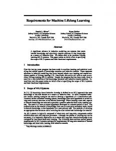
We now further elaborate on eigenvalues, which are a special set of scalars associated with a linear system of equations that are sometimes also known as characteristic roots, proper values, or latent roots. Eigenvalues and eigenvectors of a matrix contain the distances or similarities between the data points. They provide information on the principal directions of the data and therefore provide a means of understanding the spread of the data. We are able to observe in Figure ?? the explanation of the data directions of a 100 multidimensional point Gaussian, using the first two eigenvectors (which are the first two principle directions). 10 8 6 4

X2

2 0 −2 −4 −6 −8 −10 −10

−5

0 X1

5

10

Figure 2.5: Principle directions on a Gaussian.

Given a matrix A, we have the real number λ and the vector x that are a corresponding eigenvalue and eigenvector of A iff Ax = λx. The matrix A only changes the length of x and not its direction (Figure 2.6).


19

Figure 2.6: The vector’s length is simply scaled by λ and A.

The eigenvalue and eigenvector obey the quotient known as the Rayleigh quotient (although this is also true for any vector) x0 x x0 Ax = λ = λ. x0 x x0 x We consider the optimisation problem max x

x0 Ax . x0 x

(2.6)

As it is invariant to rescaling of x we are able to maximise the denominator with the imposed constraint x0 x = 1. Solving the Lagrangian we obtain the following L(x, λ) = x0 Ax − λ(x0 x − 1) and taking derivatives with respect to x gives ∂L = Ax − λx ∂x setting equal to zero gives Ax = λx. We assume that the eigenvectors are normalised. Therefore the eigenvector corresponding to the largest eigenvalue gives the solution of the maximisation optimisation in equation (2.6). We are guaranteed a solution for the optimisation problem as we seek the maximisation, and similarly with minimisation since x is non zeros and finite. For symmetric matrices the eigenvectors corresponding to distinct eigenvalues are orthogonal, as if µ, z are a second eigenvalue and eigenvector pair Az = µz with µ 6= λ,

20


we have that λ hx, zi = hAx, zi = (Ax)0 z = x0 A0 z = x0 Az = µ hx, zi implying that hx, zi = 0. This means that if A is a ` × ` symmetric matrix, it can have at most ` distinct eigenvalues. The transformation, given a normalised x, A˜ = A − λxx0 is known as deflation, this leaves x as an eigenvector but reduces the corresponding ˜ = Ax − λxx0 x = 0. Since the eigenvectors corresponding to eigenvalue to zero as Ax distinct eigenvalues are orthogonal, the remaining eigenvalues of A stay unchanged. We are able to find ` orthonormal eigenvectors by computing the eigenvector for the largest positive eigenvalue and then deflating. Eigen-decomposition of a symmetric matrix A is the process of forming a matrix V with the orthonormal eigenvectors as columns and a diagonal matrix with the corresponding eigenvalues Λ where Λii = λi , i = 1, . . . , `. This gives us V V 0 = V 0 V = I and AV = V Λ. The computed eigenvalues are known as A’s eigenspectrum. Where we usually assume that the eigenvalues are in decreasing order λ1 ≥ λ2 ≥ . . . ≥ λ` .

2.4

Support Vector Machines

We briefly describe a method known as Support Vector Machines, which will be encountered in the application part of the thesis. This method attempts to create a computationally efficient way of learning the separating hyperplanes, for a classification problem, in a high dimensional feature space. Recall the Lagrangian of the hyperplane optimisation problem in Section 2.1.1 `

X 1 L(w, α, b) = kwk2 − αi yi (hw, xi i + b) − 1 2

(2.7)

i=1

with derivatives w =

` X

αi yi xi

(2.8)

i=1 ` X i=1

αi yi = 0.

(2.9)


21

The Karush-Kuhn-Tucker complementary conditions from optimisation theory (see Appendix A.4) give information about the structure of the solution. These conditions show that the optimal solution must satisfy αi [yi (hxi , wi + b) − 1] = 0,

i = 1, . . . , `.

Therefore the weight vector only involves the non-zero αi , which are called Support Vectors, that correspond to the data points that lie on the supporting hyperplanes. i.e. their functional margin is one. The remaining samples are irrelevant as the hyperplane is entirely determined by the examples closest to it. Substituting equations (2.8) and (2.9) into equation (2.7) gives us the dual optimisation problem of which we maximise in respect to the dual variables αi (see Appendix B.1.1 for full derivation), we obtain

max W (α) = α

` X

αi −

i=1

subject to

P`

` 1 X αi αj yi yj κ(xi , xj ) 2 i,j=1

i=1 αi yi

= 0 and αi ≥ 0 i = 1, . . . , `.

The decision function in feature space is therefore h(x) = sgn

= sgn

` X i=1 ` X

! yi αi hφ(xi ), φ(x)i + b ! yi αi κ(xi , x) + b .

i=1

Although in practice it may be the case that a separating hyperplane might not exist due to overlapping of classes. We introduce a slack variable into our notation to allow for some sample violation of the margin conditions ξi ≥ 0 i = 1, . . . , `

(2.10)

and relax the constraint to yi (hxi , wi + b) ≥ 1 − ξi ,

i = 1, . . . , `.

(2.11)

Therefore our new relaxed optimisation where we control both the classifier capacity and the sum of the slacks is `

1 1 X 2 min f (kwk) = kwk2 + C ξi 2 2 kwk i=1

s.t. ξi ≥ 0, C > 0

22


and subject to constraints (2.10) and (2.11). The constant C controls the trade-off between minimising the number of errors and maximising the margin. The Lagrangian for the new optimisation problem is `

`

i=1

i=1

1 X 2 X 1 L(w, α, b, ξ) = kwk2 + C ξi − αi (yi (hw, xi i + b) − 1 + ξi ) 2 2

where the only difference is that now we need to take the partial derivative in respect to the slack variables ξ ∂L = Cξ − α = 0. ∂ξ Resubstituting the relations obtained into the primal formulations obtains the following dual objective function to maximise (Appendix B.1.2 for full derivation)

max W (α) = α

subject to

2.5

` X i=1

P`

` 1 X 1 αi − yi yj αi αj κ(xi , xj ) + δij 2 C

i=1 αi yi

(2.12)

i,j=1

= 0, i = 1, . . . , ` and 0 ≤ αi ≤ C.

Summary

In this chapter we review kernel methodology and its motivation for learning non linearly separable data, also showing that by applying the kernel trick we are able to overcome the explicit embedding of the data into feature space. A process that becomes rapidly too computationally expensive to perform. We show how partial Gram-Schmidt orthonormalisation can be used in order to create a matrix composed of linearly independent vectors. This process will later be utilised to create an invertible matrix from a kernel matrix. We present eigen analysis, which can be used as a means of understanding the spread of the data. The chapter is concluded with describing a commonly used method, Support Vector Machines, for learning the most efficient separating hyperplanes for a classification problem.

Chapter 3

Semantic Models “I have always wished for a computer that would be as easy to use as my telephone. My wish came true. I no longer know how to use my telephone.” - Bjarne Stroustrup Semantics1 is the study of meaning and the change of meaning. This chapter will introduce several methods for creating semantic models from data. This process would enable use to both examine the ability of dimension reduction and the extraction of relevant features of the data, hopefully leading to an improvement when used in conjunction with a learning algorithm. We present two genres of semantic representation, starting with several methods based on eigenanalysis and conclude with a different approach based on probability.

3.1

Semantic Representation by Linear Regression

We will consider in the following how feature spaces derived from solving the eigenvalue problem could be used to enhance regression accuracy. Least squares is the procedure of finding the best fitting curve to data, such that the error of the sum of the squares of the points offsets from the curve is minimised. In the process of the optimisation of least squares regression we seek a vector w such that it solves min kXw − yk2 w

where X contains as rows the feature vectors of the samples and y contains the outputs. We are able to consider a more general multivariate regression by taking w and y to be matrices and the norm to be the Frobenius norm min kXW − Yk2F . W

1

From the Greek word semantikos, or ‘significant meaning’.

23

24

Chapter 3 Semantic Models

Principal Component Analysis (PCA) is the process of examining the direction of maximum variance within the data. We seek linear combinations of the data that preserves the characteristics of the data while finding directions with maximum variance. The PCA can be solved by the following optimisation problem w0 X0 Xw,

maxw

subject to kwk = 1 where kwk is the first eigenvector and X is centred (i.e. the origin is moved to the centre of the mass of X). We consider the usage of the features returned from PCA. Using the first k eigenvectors of X0 X as our features and leaving the outputs Y unchanged. This translates into two stages; performing PCA and regressing in the feature space given by the first k principal directions and then minimising the least square error between the projected data and the response. This is also known as Principal Component Regression (PCR). Let X = VΣ0 U0 be the Singular Value Decomposition (SVD)2 of X, therefore the data matrix is now represented as XUk where Uk contains the first k columns of U. We describe the least squares solution, which will be used in the next sections. In the following we obtain the least squares regression problem min kXUk B − Yk2F = min kVΣ0 U0 Uk B − Yk2F B

B

where we are able to multiply by an orthogonal matrix V0 as this does not effect the norm, giving min kV0 VΣ0 U0 Uk B − V0 Yk2F = min kΣ0k B − V0 Yk2F B

B

Σk is the matrix containing the first k columns of Σ and similarly let Vk contain the first k columns of V. We find that Σ0k B = V0 Y ¯ −1 V0 Y. B = Σ k k ¯ −1 is the symmetric square matrix containing the first k columns inverse of Σk . Where Σ k ¯ −10 , allowing Following the singular value decomposition of X we find that Vk = XUk Σ k

us to express B as ¯ −2 U0 X0 Y. B=Σ k k Showing that the components are computed as an inner product between the features and the data matrix weighted by the inverse of the eigenvalues. The critical measure of the different coordinates is their covariance with the data matrix X0 Y suggesting that 2

The Singular Value Decomposition is a widely used technique to decompose a matrix into several component matrices, exposing properties of the original matrix. Using the SVD, we can determine the rank of matrix, quantify the sensitivity of a linear system to numerical error, or obtain an optimal lower-rank approximation to the matrix.


25

Algorithm 4 The PLS feature extraction algorithm input: Data matrix X ∈ R`×N , dimension k and target vectors Y R`×m .

∈

X1 = X for j = 1, . . . , k do let uj , σj be the first singular vector/value of X0j Y, uj u0 X0 Xj Xj+1 = Xj I − u0 Xj0 Xjj uj j

j

end for Output: Feature directions uj , j = 1, . . . , k. rather than seeking directions that give maximum variance we should seek direction that maximise the covariance. In the following section we will investigate an approach for seeking directions that give maximum covariance.

3.1.1

Partial Least Squares

Partial Least Squares (PLS) was developed by Herman Wold during the 1960’s in the field of econometrics3 . It offers an effective approach to solving problems with training data that has few points but high dimensionality, by first projecting the data into a lower-dimensional space and then utilising a least squares regression model. This problem is common in the field of Chemometrics4 where PLS is regularly used. PLS is a flexible algorithm that was designed for regression problems, though it can be used for classification by treating the labels {+1, −1} as real outputs. Alternatively it can also be stopped after constructing the low-dimensional projection. The resulting features can then be used in a different classification or regression algorithm. The procedure for PLS feature extraction is shown in Algorithm 4. The algorithmic procedure iteratively takes the first singular vector ui of the matrix X0i Y, and then deflates the matrix Xi to obtain Xi+1 . The deflation is done by projecting the columns of Xi into the space orthogonal to Xi ui Xi+1 =

Xi ui u0 X0 I− 0 0 i i ui Xi Xi ui

Xi = Xi

ui u0 X0 Xi I − 0 i0 i ui Xi Xi ui

.

Since u is a singular vector of matrix X0 Y which gives the recursive step for u u = X0 j Yj Y0 j Xj u. 3 Econometrics is the application of statistical and mathematical methods in the field of economics to test and quantify economic theories and the solutions to economic problems. 4 Chemometrics is the application of statistics to the analysis of chemical data (from organic, analytical or medicinal chemistry) and design of chemical experiments and simulations.

26


We can deflate Y to its residual but since this does not affect the correlations found as the deflation removes components in the space spanned by X0 j u, to which Xj+1 is now orthogonal to. Therefore the recursive step renders the deflation of Y with no affect on the outputs. The difficulty with this simple description is that the feature directions uj are defined relative to the deflated matrix, hence we would need the deflated matrices in order to get the final feature vectors. We would like to be able to compute the PLS features directly from the original feature vector such that we would be able to apply the feature directions to a test set. If we now consider a test point with feature vector φ (x) the transformations that we perform at each step should also be applied to φ1 (x) = φ (x) to create a series of feature vectors φj+1 (x)0 = φj (x)0 I − uj p0j , where pj =

X0j Xj uj . u0j X0j Xj uj

This is the same operation that is performed on the rows of Xj in Algorithm 4. We can now write 0

0

φ (x) = φk+1 (x) +

k X

φj (x)0 uj p0j .

j=1

ˆ (x) has components The feature vector that is needed for the regression φ ˆ (x) = φj (x)0 uj φ

k j=1

,

since these are the projections of the residual vector at stage j onto the next feature vector uj . Rather than computing φj (x)0 iteratively, consider we use the inner products between the original φ (x)0 and the feature vectors uj stored as the columns of the matrix U: φ (x)0 U = φk+1 (x)0 U +

k X

φj (x)0 uj p0j U

j=1 0

ˆ (x)0 P0 U, = φk+1 (x) U + φ where P is the matrix whose columns are pj , j = 1, . . . , k. Finally, it can be verified that u0i pj = δij

for i ≤ j. Hence, for s > j, (I − us p0s ) uj = uj , while I − uj p0j uj = 0, so we can write

0

0

φk+1 (x) uj = φj (x)

k Y i=j

I − ui p0i uj = 0, for j = 1, . . . , k.


27

It follows that the new feature vector can be expressed as ˆ (x)0 = φ (x)0 U P0 U −1 . φ These feature vectors can now be used in conjunction with a learning algorithm. We can compute the regression coefficients as: −1 0 W = U P0 U C, where C is the matrix with columns cj =

3.1.2

Y0 Xj uj . u0j X0j Xj uj

Kernel Partial Least Squares

In this section we set out the kernel PLS algorithm and describe its feature extraction stage. The kernel PLS is the process of applying the dual PLS procedure in kernel feature space, which is given in Algorithm 5. The vector βi is a rescaled dual representation of Algorithm 5 Pseudocode for kernel-PLS Input: Data S = x1 , . . . , xl dimension k target outputs Y ∈ Rl×m Kij = κ (xi , xj ) K1 = K Yˆ = Y for i = 1, . . . , k do βi = first column of Yˆ normalise βi repeat βi = Y Y 0 Ki βi normalise βi until convergence (of eigenvectors) τi = Ki βi ci = Yˆ 0 kττiik2 Yˆ = Yˆ − τi c0i τ τ0 τ τ0 Ki+1 = I − kτii ki2 Ki I − kτii ki2 end for B = [βi , . . . , βk ] T = [τi , . . . , τk ] α = B(T KB)−1 T 0 Y Output: Dual regression coefficients α the primal vectors ui : ai ui = X0i βi ,

(3.1)

28


the rescaling arises because of the different point at which the renormalising is performed in the dual. Let τj = aj Xj Uj be the rescaled dual representation of the output vector cj . Therefore pj can be written as pj =

aj X0j τj X0j Xj uj = . u0j X0j Xj uj τj0 τj

As in the dual setting we compute β in the recursive step β = Yj Yj0 Xj X0j β, we are no longer multiplying by the next Xj+1 and therefore not removing the orthogonal elements from the deflation of Y. Hence the deflation of Y in the dual is necessary as this would change the overall output. Since τj τi = aj ai U0j X0j Xi Ui = 0 for j > i, τ are orthogonal, this furthermore means

τi τ 0 I− 0 i τi τi

τj = τj

implying X0j τj = X0 τj . We can now express the primal matrix P0 U in terms of the dual variables as P0 U = diag (a) diag τi0 τi

−1

T0 XX0 Bdiag (a)−1

= diag (a) diag τi0 τi

−1

T0 KBdiag (a)−1 .

Here diag (τi0 τi ) is the diagonal matrix with entries diag (τi0 τi )ii = τi0 τi , where τi = Ki βi . Finally, again using the orthogonality of Xj uj to τi , for i < j, we obtain cj =

Yj0 Xj uj Y0 Xj uj Y 0 τj = = a , j 0 u0j X0j Xj uj u0j X0j Xj uj τj τj

making C = Y0 Tdiag τi0 τi

−1

diag (a) .

Putting the pieces together we can compute the dual regression variables as α = B T0 KB

−1

T0 Y.

It is tempting to assume like Rosipal et al. (2003) that a dual representation of the PLS features is then given by B T0 KB

−1

,

but in fact −1 −1 −1 0 U P0 U = X0 Bdiag (a)−1 diag (a) diag τi0 τi T KBdiag (a)−1


29

so that the dual representation is B T0 KB

−1

−1 diag (a)−1 diag τi0 τi = B T0 KB diag τi0 τi diag (a)−1 .

PLS could be thought of as a method which looks for directions that are good at distinguishing the different labels, as it selects feature directions that are useful for the task at hand using one view of the object with the label as the corresponding pair. In the following section we introduce canonical correlation analysis which is similar to PLS though selects the feature directions that are useful for the task using two views of an object.

3.2

Introduction to Canonical Correlation Analysis

Canonical Correlation Analysis (CCA) (Hotelling, 1936) can be seen as the problem of finding basis vectors for two sets of variables such that the correlation of the projections of the variables onto these basis vectors are mutually maximised. While ordinary correlation analysis is dependent on the coordinate system in which the variables are described, CCA is invariant with respect to an affine transformation5 of the variables. CCA is a method of identifying linear relationships between two multidimensional variables. CCA can be also seen as using complex labels as a way of guiding feature selection towards the underlying semantics. CCA makes use of two views of the same semantic object to extract a representation of the semantics. We seek a linear combination x = wx0 x and y = wy0 y, where wx and wy are some linear transformation, such that the correlation between the projection of the variables onto the basis vectors is maximised. CCA will be discussed in more detail in the following chapter.

3.2.1

Example

We give an example to show where ordinary correlation can fail to identify the correlation in a given system, justifying the canonical correlation approach. Consider two normally distributed two-dimensional variables x and y with unit variance. Let z = x1 + x2 = y1 + y2 , as plotted in Figure 3.1. Let u, v be scalars such that we are able to express x and y as (x1 , x2 ) = (y1 , y2 ) = 5

z z2 2

z +u 2 z + v, − v . 2 − u,

An affine transformation is any transformation that preserves collinearity and ratios of distances.

30


Figure 3.1: Two normally distributed two-dimesional variables.

Assume that u, v and z are linearly independent and that their expectation is E(z) = E(u) = E(v) = 0, and assume that var(z) = 2. We first compute the ordinary correlation between x1 and y1 . corr(x1 , y1 ) = = = = = =

cov(x1 , y1 ) p

var(x1 )var(y1 ) E(x1 y1 ) − E(x1 )E(y1 ) z z E −u +v 2 22 z uz vz E − uv − + 4 2 2 2 1 1 z E − E(u)E(v) − E(u)E(z) + E(v)E(z) 4 2 2 2 z 1 E = E(z 2 ). 4 4

Computing the expectancy of E z 2 as E(z 2 ) = var(z) − E(z)2 = 2 − 0 = 2 which gives corr(x1 , y2 ) =

1 2


31

and similarly for the remaining correlation, obtaining us the weak correlation in Table 3.1. Table 3.1: Ordinary Correlation Values

y1 y2

x1 0.5 0.5

x2 0.5 0.5

CCA however is able to find the coordinate system that is optimal for the correlation analysis, we are able to find a linear combination such that perfect linear relationship exists. Therefore x1 = y1 and x2 = y2 , and assume that var(u) = var(v) = 12 . We first compute the ordinary correlation between x1 and y1 . corr(x1 , y1 ) =

cov(x1 , y1 ) p

var(x1 )var(y1 )

= E(x21 ) − E(x1 )E(x1 ) z z = E −u −u 2 22 uz z + u2 − 2 = E 4 2 2 z = E + E(u2 ) = 4 1 1 = + = 1. 2 2 We compute the ordinary correlation between x1 and y2 . corr(x1 , y1 ) = = = = = =

cov(x1 , y2 ) p

var(x1 )var(y2 ) E(x1 y2 ) − E(x1 )E(y2 ) z z E −u +u 2 22 z uz uz 2 E −u − + 4 2 2 2 z E − E(u2 ) 4 1 1 − = 0. 2 2

Giving us the correlation values in Table 3.2.

32


Table 3.2: Canonical Correlation Values

y1 y2

3.3

x1 1 0

x2 0 1

Probabilistic Approach to Semantic Representation

The idea of generating a feature representation and associated kernel from a probabilistic model of our data is very appealing. It suggests a practical way of incorporating domain knowledge while still allowing us to use powerful non-parametric methods such as support vector machines. In this sense we can hope to get the best of both worlds: use the probabilistic models to create a feature representation that captures our prior knowledge of the domain, while leaving open the actual analysis methods to be used. The most popular method of deriving a feature vector from a probabilistic model is known as the Fisher score or Fisher kernel. This method creates a feature vector from a smoothly parametrised probabilistic model by computing the gradients of the loglikelihood of a data item around the chosen parameter setting. This can be seen as estimating the direction the model would be deformed if we were to incorporate the data item into the parameter estimation. We now give formal definitions of these concepts. Definition 3.1. [Fisher score and Fisher information matrix] The log-likelihood of a data item x with respect to the model m(θ0 ) for a given setting of the parameters θ0 is defined to be log Lθ0 (x), where for a given setting of the parameters θ0 the likelihood is given by L0θ (x) = P (x|θ0 ) = Pθ0 (x) . Consider the vector gradient of the log-likelihood g (θ, x) =

∂ log Lθ (x) ∂θi

N . i=1

The Fisher score of a data item x with respect to the model m(θ0 ) for a given setting of the parameters θ0 is g θ0 , x .


33

The Fisher information matrix with respect to the model m(θ0 ) for a given setting of the parameters θ0 is given by h 0 i IM = E g θ 0 , x g θ 0 , x ,

(3.2)

where the expectation is over the generation of the data point x according to the data generating distribution. The Fisher score gives us an embedding into the feature space RN and hence immediately suggests a possible kernel. The matrix IM can be used to define a weighted inner product in that feature space.

Definition 3.2. [Fisher kernel] The invariant6 Fisher kernel with respect to the model m(θ0 ) for a given setting of the parameters θ0 is defined as 0 0 κ(x, z) = g θ0 , x I−1 M g θ ,z . The expectation in equation (3.2) is not computable except for simple models. Therefore it is common practice to replace I−1 M with the identity matrix. This is referred to as the practical Fisher kernel, which is defined as 0 κ(x, z) = g θ0 , x g θ0 , z .

We will follow the standard route of restricting ourselves to the practical Fisher kernel. Notice that this kernel may give a small norm to very typical points, while atypical points may have large derivatives and so a correspondingly large norm. There is, therefore, a danger that the inner product between two typical points can become very small, despite their being similar in the model. This effect can be overcome by normalising the kernel. Another way to use the Fisher score that does not suffer from the problem described above is to use the Gaussian kernel based on distance in the Fisher score space ! kg θ0 , x − g θ0 , z k2 κ(x, z) = exp − . 2σ 2

In Algorithm7 6 we quote from Shawe-Taylor and Cristianini (2004) the derived Fisher kernel for Hidden Markov Model (HMM), where the pseudocode is given for evaluating the Fisher scores for the emission probabilities. 6

The Fisher kernel is invariant in respect to the length of gradient vector. i.e. we can multiply the gradient vector by any positive scalar and this will not change the kernel. 7~ A Creates a row vector out of the entries of matrix A by concatenating its rows.

34


Definition 3.3. [Hidden Markov model] A hidden Markov model (HMM) M comprises a finite set of states A with an initial state aI , a final state aF , a probabilistic transition function PM (a|b) giving the probability of moving to state a given that the current state is b, and a probability distribution P (σ|a) over symbols σ ∈ Σ ∪ {ε} for each state a ∈ A.

Algorithm 6 Pseudocode to compute the Fisher scores for the fixed length Markov model Fisher kernel. Input: Symbol string s, state transition probability matrix PM (a|b), initial state probabilities PM (a) = PM (a|a0 ) and conditional probabilities P (σ|a) of symbols given states. Assume p states, 0, 1, . . . , p. score (:, :) = 0; f orw (:, 0) = 0; back (:, n) = 1; f orw (0, 0) = 1; P rob = 0; for i = 1 : n do for a = 1 : p do f orw (a, i) = 0; for b = 0 : p do f orw (a, i) = f orw (a, i) + PM (a|b) f orw (b, i − 1) ; end for f orw (a, i) = f orw (a, i) P (si |a) ; end for end for for a = 1 : p do P rob = P rob + f orw (a, n) ; end for for i = n − 1 : 1 do for a = 1 : p do back (a, i) = 0; for b = 1 : p do back (a, i) = back (a, i) + PM (b|a) P (si+1 |b) back (b, i + 1) ; end for orw(a,i) score (a, si ) = score(a,siP)+back(a,i)f ; (si |a)P rob for σ ∈ Σ do orw(a,i) score (a, σ) = score (a, σ) − back(a,i)f ; P rob end for end for end for Output: Fisher score = score ~


3.4

35

Summary

In this chapter we review how semantic models can be created by analysing the spread of the data or its affect on a system. Having introduced several approaches for creating semantic models, we return to the method introduced in Section 3.2 for creating a semantic model using two views of an object. The following chapter analyses the main investigated technique of canonical correlation analysis and its kernel variant.

Chapter 4

Canonical Correlation Analysis; A Detailed Review “Computers are useless. They can only give you answers.” - Pablo Picasso

4.1

Canonical Correlation Analysis

Proposed by Hotelling in 1936, Canonical Correlation Analysis (CCA) is a technique for finding pairs of basis vectors that maximise the correlation between the projections of paired variables onto their corresponding basis vectors. Correlation is dependent on the chosen coordinate system, therefore even if there is a very strong linear relationship between two sets of multidimensional variables this relationship may not be visible as a correlation (see example in Section 3.2.1). CCA seeks a pair of linear transformations one for each of the paired variables such that when the variables are transformed the corresponding coordinates are maximally correlated. Consider a pair of multivariate random vectors of the form (x, y) with zero mean. Suppose we are given a sample of ` instances S = ((x1 , y1 ), . . . , (x` , y` )) of (x, y), let Sx denote (x1 , . . . , x` ) and similarly Sy to denote (y1 , . . . , y` ). We can consider defining a new coordinate for x by choosing a direction wx and project x onto that direction x → hwx , xi . If we do the same for y by choosing a direction wy , we obtain a sample of the new x coordinate, let Sx,wx = (hwx , x1 i , . . . , hwx , x` i) with the corresponding values of the new y coordinate being Sy,wy = (hwy , y1 i , . . . , hwy , y` i). 37

38

Chapter 4 Canonical Correlation Analysis; A Detailed Review

We choose wx and wy such that the correlation between the two vectors is maximised. Hence max ρ = corr(Sx,wx , Sy,wy )

Sx,wx , Sy,wy = p . kSx,wx kkSy,wy k

wx ,wy

We are able to rewrite the canonical correlation expression as ˆ E[hw x , xi hwy , yi]

max ρ =

q

wx ,wy

2 ˆ 2 ˆ E[hw x , xi ]E[hwy , yi ]

ˆ 0 xy0 wy ] E[w x

=

q

ˆ 0 yy0 wy ] ˆ 0 xx0 wx ]E[w E[w y x 0 ]w ˆ wx0 E[xy y

=

q

.

(4.1)

0 ]w w0 E[yy 0 ]w ˆ ˆ wx0 E[xx x y y

Observe that the empirical covariance matrix of (x, y) is equal to its empirical expectation " ˆ E

x

!

y

x

!0 #

" ˆ =E

y

xx0 xy0 yx0 yy0

#

" ˆ =E

Cxx Cxy

#

Cyx Cyy

= C.

(4.2)

The total covariance matrix C is a block matrix with the within-sets covariance matrices 0 . Hence, we are able to Cxx , Cyy and the between-sets covariance matrices Cxy = Cyx

rewrite equation (4.1) as max ρ = p

wx ,wy

wx0 Cxy wy . wx0 Cxx wx wy0 Cyy wy

(4.3)

Observe that equation (4.3) is not affected by the re-scaling of wx or wy either together or independently. For example, replacing wx by αwx will give the quotient αwx0 Cxy wy q

α2 wx0 Cxx wx wy0 Cyy wy

=p

wx0 Cxy wy . wx0 Cxx wx wy0 Cyy wy

As the choice of re-scaling is arbitrary, the CCA optimisation problem in equation (4.3) is equivalent to maximising the numerator subject to wx0 Cxx wx = 1 wy0 Cyy wy = 1.


39

The corresponding Lagrangian to the optimisation problem is L(λx , λy , wx , wy ) = wx0 Cxy wy −

λy λx 0 (wx Cxx wx − 1) − (wy0 Cyy wy − 1). 2 2

Taking derivatives in respect to wx and wy we obtain equations ∂L ∂wx ∂L ∂wy

= Cxy wy − λx Cxx wx = Cyx wx − λy Cyy wy .

Subtracting wy0 times the second equation from wx0 times the first gives wx0 Cxy wy − wx0 λx Cxx wx − wy0 Cyx wx + wy0 λy Cyy wy = 0 λx wx0 Cxx wx − λy wy0 Cyy wy = 0 which together with the constraints implies that λy −λx = 0. Let λ , λx = λy , therefore Cxy wy − λCxx wx = 0

(4.4)

Cyx wx − λCyy wy = 0 following the proof in Appendix B.2.1 we show that ρ = λ. Assuming C is invertible we have wy =

−1 C w Cyy yx x λ

(4.5)

and so substituting in equation (4.4) gives −1 Cxy Cyy Cyx wx = λ2 Cxx wx .

(4.6)

This leaves us with a generalised eigenproblem of the form Ax = λBx, where A and B are symmetric matrices. We can now find the coordinate system that optimises the correlation between corresponding coordinates by first solving for the generalised eigenvectors of equation (4.6) to obtain the sequence of wx ’s and then using equation (4.5) to find the corresponding wy ’s (Borga, 1998). As we have assumed C to be invertible we are able to rewrite equation (4.6) as a standard eigenproblem of the form Ax = λx. In order to ensure that A is symmetric we first decompose the covariance matrices, as they are symmetric positive definite, using Cholesky decomposition 0 Cxx = Rxx Rxx

40


where Rxx is an upper triangular matrix. Let ux = Rxx wx we can rewrite equation (4.6) as −1 −1 0 Cxy Cyy Cyx Rxx ux = λ2 Rxx ux 0

−1 −1 −1 Rxx Cxy Cyy Cyx Rxx ux = λ2 ux

which ensures a symmetric standard eigenproblem. Since the computed eigenvalues lie in the interval of [−1, +1] we discard half of the spectrum as they are paired " λ

u v

#

" ↔ −λ

u

#

-v

we are only interested in half of the spectrum where the eigenvectors correspond to the largest eigenvalues which in turn identify the strongest correlations.

4.2

Kernel Canonical Correlation Analysis

We may find that due to its linearity, canonical correlation analysis may not extract useful descriptors from the data, since the correlation will exist in some non linear relationship. The kernelising of CCA offers an alternate solution by first projecting the data into a higher dimensional feature space φ : x = (x1 , . . . , xn ) → φ(x) = (φ1 (x), . . . , φN (x)) (N ≥ n) before performing CCA in the new feature space. The data appears as inner products between the samples in the kernel, therefore giving a further advantage as the number of tuneable parameters and updating time does not depend on the number of attributes being used. Let φa be the projection for x and φb the projection for y φa : x → φa (x) φb : y → φb (y). Hence let κa and κb be the corresponding kernel function for the two feature projections. As we wish to solve the problem in the dual formulation we create a matrix X whose rows are the vectors φa (xi ), i = 1, . . . , ` and similarly a matrix Y with rows φb (yi ). Using the covariance matrix in equation (4.2) we are able to define the covariance matrix of the projected data points as Cxx = X0 X Cxy = X0 Y


41

and similarly with Cyy and Cyx . The covariance matrix will be identical to the covariance matrix in equation (4.2) only if a linear mapping will be used, hence N = n. The weights wx and wy can be expressed as a linear combination of the training examples wx = X0 α wy = Y0 β. Substituting into equation (4.3) gives max ρ = p α,β

α0 XX0 YY0 β (α0 XX0 XX0 α)(β 0 YY0 YY0 β)

.

(4.7)

Given the kernel functions κa and κb let Ka and Kb be the kernel matrices corresponding to the two representations of the data. Substituting into equation (4.7) α0 Ka Kb β max ρ = q . α,β α0 Ka2 αβ 0 Kb2 β

(4.8)

The CCA optimisation problem in equation (4.8) is now represented in the dual form. Observe that as with the primal form in equation (4.3), equation (4.8) is not affected by the rescaling of α and β either together or independently. Hence the Kernel CCA optimisation problem is equivalent to maximising the numerator subject to α0 Ka2 α = 1 β 0 Kb2 β = 1. The corresponding Lagrangian is L(λa , λb , α, β) = α0 Ka Kb β −

λa 0 2 λb 0 2 (α Ka α − 1) − (β Kb β − 1) 2 2

taking derivatives in respect to α and β we obtain ∂L ∂α ∂L ∂β

= Ka Kb β − λa Ka2 α = 0

(4.9)

= Kb Ka α − λb Kb2 β = 0.

(4.10)

Subtracting β 0 times the second equation from α0 time the first gives α0 Ka Kb β − α0 λa Ka2 α − β 0 Kb Ka α + β 0 λb Kb2 β = 0 λa α0 Ka2 α − λb β 0 Kb2 β = 0 which together with the constraints implies that λa − λb = 0. Let λ , λa = λb , and by following the proof for primal CCA in Appendix B.2.1 it is easy to show that ρ = λ for the dual case. Considering the case where the kernel matrices Ka and Kb are invertible,

42


we have β = =

Kb−1 Kb−1 Kb Ka α λ −1 Kb Ka α λ

substituting in equation (4.10) gives Ka Kb Kb−1 Ka α − λ2 Ka Ka α = 0. Hence Ka Ka α − λ 2 Ka Ka α = 0 or Iα = λ2 α.

(4.11)

We are left with a standard eigenproblem of the form Ax = λx. We can deduce from equation (4.11) that λ = ±1 for every vector α, hence we can choose the projections α to be unit vectors ji i = 1, . . . , l while β are the columns of Kb−1 Ka . This is an interesting and somewhat surprising result as it shows that when we assume the kernel matrices Kb or Ka to be invertible, perfect correlations can be formed. This stats that we are able to find perfect correction in the kernel representation. Since kernel methods provide high dimensional representations such independence is not uncommon. It is therefore clear that a naive application of CCA in kernel defined feature space will not provide useful results.

4.3

Statistical Analysis of Canonical Correlation Analysis

As observed in the previous section, naive application of CCA in kernel space will be likely to produce perfect correlations between the two views. These correlations can therefore fail to distinguish between spurious features and those that capture the underlying semantics. Here we follow the outline given in (Shawe-Taylor and Cristianini, 2004) and provide a theoretical analysis of Kernel CCA in order to provide a better understanding of the technique’s stability. For this we use Rademacher complexity (Appendix A.6) to obtain an error bound for a new data sample. The theoretical analysis justifies kernel CCA regularisation proposed by (Bach and Jordan, 2002) but indicates that a different normalisation of the features should be used. The use of regularisation aims to remove the spurious correlations mentioned above. Consider two multivariate projections φa (x) and φb (x) of a random object x. Given the projection direction wa and wb we would like to capture the notion that the features


43

from one view are almost identical to the features from the second view. The function1 gwa ,wb (x) = kwa0 φa (x) − wb0 φb (x)k2 , 0 2 0 2 ˆ ˆ subject to E[kw a φa (x)k ] = 1 and E[kwb φb (x)k ] = 1 measures this property. If

gwa ,wb (x) ≈ 0 we are able to deduce that the feature that can be obtained from the first view is almost identical to feature obtained from the second. Such pairs of features are able to capture the underlying semantic properties of the data that are present in both views of the object. We obtain a stability analysis of the function by viewing gwa ,wb (x) as a regression function with special structure, attempting to learn the constant zero function. In order to apply the Rademacher generalisation bound, we must first compute the empirical expected value of gwa ,wb (x) 0 0 2 0 2 0 2 ˆ ˆ ˆ E[kw a φa (x) − wb φb (x)k ] = E[kwa φa (x)k ] + E[kwb φb (x)k ]

ˆ w0 φa (x), w0 φb (x) ] −2E[ a b

= 2(1 − wa0 Cab wb ) where

n

Cst =

1X φs (xi )φt (xi )0 , n

for s, t ∈ {a, b}.

i=1

We represent gwa ,wb (x) as a linear function fˆ(x) in an appropriately defined feature ˆ be the mapping into the feature space F given by space F . Let φ √ ~ b (x)0 ], ~ a (x)0 , φb (x)φ ~ b (x)0 , 2φa (x)φ ˆ φ(x) = [φa (x)φ and the weight vector

√ ˆ = [wa~wa0 , wb~wb0 , − 2wa~wb0 ] w

ˆ realises the function gwa ,wb (x) see Appendix B.2.2 for proof. It can be verified that w ˆ in the feature space defined by φ(x) D

E ˆ ˆ φ(x) w, = (wa0 φa (x))2 + (wb0 φb (x))2 − 2wa0 φa (x)wb0 φb (x) = kwa0 φa (x) − wb0 φb (x)k2 .

ˆ can be computed (see Appendix B.2.3) It is interesting to observe that the norm of w as ˆ = kwa k2 + kwb k2 , kwk showing that the combined norm is just the summation of the square of the individual ˆ is therefore given by (see norms. The kernel κ ˆ corresponding to the feature mapping φ 1

We use the k · k representation as in the following section we will be working with matrices.

44


Appendix B.2.4) κ ˆ (x, z) = (κa (x, z) + κb (x, z))2 .

4.3.1

k-dimensional Analysis

The analysis considered so far only concerns projections into a 1-dimensional space. In practice we will project into a k-dimensional space using the orthogonal eigenvectors corresponding to the top k correlation directions as our projection vectors. In order to handle this case we introduce the matrix Wa whose columns are the first k vectors wa1 , . . . , wak , and Wb with the corresponding wb1 , . . . , wbk . We denote ga,b (x) , gWa ,Wb (x) where k X

gWa ,Wb (x) =

gwai ,wi (x) b

i=1

= kWa φa (x) − Wb φb (x)k2 Theorem 4.1. Fix A and B in R+ . If we obtain features given by (wa )i , (wb )i i = 1, . . . , k with kwai k ≤ A and kwbi k ≤ B with correlations ρi on a paired training set S of size n in the feature space defined by the kernels κa and κb , then with probability greater than 1 − δ over the generation of S, the expected value of ga,b (x) on new data is bounded by

ED [ga,b (x)] ≤

k X

4(A2

2(1 − ρi ) +

i=1

s +3R(A2 + B 2 )

v

+ `

u ` B 2 )k uX t

(κa (xi , xi ) + κb (xi , xi ))2

i=1

ln( 2δ ) 2`

where R=

max (κa (x, x) + κb (x, x)).

x∈supp(D)

See Appendix B.2.5 for proof.

4.4

Regularised Kernel Canonical Correlation Analysis

The theoretical analysis in the previous section suggests to regularise kernel CCA as it shows that the quality of the generalisation of the associated pattern function is controlled by the sum of the squares of the weight vectors norms. Hence to force non-trivial learning on the correlation we introduce a control on the flexibility of the projection mappings. In the following subsections we show two approaches for the application of regularisation.


4.4.1

45

Regularisation via Optimisation Function

We use the pattern function as formulated in Section 4.3 to represent the kernel CCA as a minimisation optimisation problem rather then a maximisation one min kKa α − Kb βk2F α,β

subject to α0 Ka2 α = 1 β

0

Kb2 β

(4.12)

= 1.

(4.13)

Instead of using two regularisation parameters for each of the weights. Let τa be the regularisation parameter for the first view and τb for the second. We use a single regularisation parameter τ = τα = τβ . Reformulating the optimisation problem as min(1 − τ )kKa α − Kb βk2F + τ (kwx k2 + kwy k2 ) α,β

equal to min(1 − τ )kKa α − Kb βk2F + τ (α0 Ka α + β 0 Kb β) α,β

and subject to equation (4.12) and (4.13). We bound the regularisation parameter to 0 ≤ τ ≤ 1 by multiplying the left parameter by (1 − τ ). The corresponding Lagrangian is L(λa , λb , α, β) = (1 − τ )2(1 − α0 Ka Kb β) + τ (α0 Ka α + β 0 Kb β) +λa (α0 Ka2 α − 1) + λb (β 0 Kb2 β − 1) taking derivatives in respect to α and β we obtain ∂L ∂α ∂L ∂β

= −2(1 − τ )Ka Kb β + 2τ Ka α + 2λa Ka2 α = 0

(4.14)

= −2(1 − τ )Kb Ka α + 2τ Kb β + 2λb Kb2 β = 0.

(4.15)

Subtracting β 0 times the second equation from α0 time the first gives τ α0 Ka α + λa = τ β 0 Kb β + λb .

Observe that we are no longer able to represent the Lagrangian multipliers in a concise form and therefore unable to solve the eigenproblem for only a single view. We proceed to solve the eigenproblem for both views combined. Assuming that the kernel matrices are invertible, we multiply equation (4.14) by

Ka−1 2

and equation (4.15) by

−1 Kb 2

which

46


gives (1 − τ )Kb β − τ α = λa Ka α (1 − τ )Ka α − τ β = λb Kb β this can be written as a general eigenproblem in the matrix form "

−τ

(1 − τ )Kb

(1 − τ )Ka −τ

#"

α β

#

" =

λa 0 0

λb

#"

Ka 0 0

#"

Kb

α

#

β

.

(4.16)

Prior to computing the correlation values we need to enforce the constraints in equations (4.12) and (4.13) as the eigenproblem in equation (4.16) will find similar solutions for rescaled α and β. Let ˆ = α βˆ =

α p αKa2 α β q βKb2 β

ˆ = 1 and βˆ0 Kb2 βˆ = 1 hold. ˆ 0 Ka2 α such that α

4.4.2

Regularisation via Optimisation Constraint

In the previous section the solution to the regularisation of the kernel CCA optimisation problem resulted in a non symmetric generalised eigenvalue problem. We are interested in finding a standard symmetric eigenproblem for a single direction, reducing the computation cost as well as reducing the size of the found solutions. in the following section we provide an alternative solution to the regularisation of the kernel CCA optimisation problem, as the resulting generalised eigenvalue problem of the previous section will be twice the size of the training set. Due to the fact that we compute the eigenproblem for both views combined. We regularise kernel CCA by adding the weight term to the constraint of the optimisation problem such that maxα,β ρ˜ = α0 Ka Kb β is now subject to (1 − τ )α0 Ka2 α + τ kwx k2 = (1 − τ )α0 Ka2 α + τ α0 Ka α = 1 (1 − τ )β 0 Kb2 β + τ kwy k2

= (1 − τ )β 0 Kb2 β + τ β 0 Kb β = 1.

Similarly to the previous section we bound τ by multiplying the left term by (1 − τ ). Observe that when maximum regularisation τ = 1 is used we are left with the kernel PLS optimisation problem for the first direction, see Appendix B.2.6.


47

The corresponding Lagrangian is L(λa , λb , α, β) = α0 Ka Kb β λa (1 − τ )α0 Ka2 α + τ α0 Ka α − 1 − 2 λb − (1 − τ )β 0 Kb2 β + τ β 0 Kb β − 1 2 Taking derivatives in respect to α and β we obtain ∂L ∂α

= Ka Kb β − λa ((1 − τ )Ka2 α + τ Ka α) = Ka Kb β − λa Ka ((1 − τ )Ka + τ I)α = 0

∂L ∂β

(4.17)

= Kb Ka α − λb ((1 − τ )Kb2 β + τ Kb β) = Kb Ka α − λb Kb ((1 − τ )Kb + τ I)β = 0.

(4.18)

Following the same procedure as in Section 4.2 we are able to find that λa = λb , let λ , λa = λb . Consider the case where the kernel matrices are invertible, we have β = =

((1 − τ )Kb + τ I)−1 Kb−1 Kb Ka α λ ((1 − τ )Kb + τ I)−1 Ka α λ

substituting into equation (4.17) gives Ka Kb ((1 − τ )Kb + τ I)−1 Ka α = λ2 Ka ((1 − τ )Ka + τ I)α multiplying both sides of the equation by Ka−1 gives Kb ((1 − τ )Kb + τ I)−1 Ka α = λ2 ((1 − τ )Ka + τ I)α.

Observe that the left component of the generalised eigenproblem is non symmetric, resulting in non orthogonal eigenvectors. In the following section we explore using partial Gram-Shmidt orthonormalisation in order to obtain an eigenproblem with symmetric matrices.

4.5

Regularised Kernel CCA with Matrix Decomposition

So far we have considered the kernel matrices as invertible, although in practice this may not be the case. The usage of large training sets may lead to computational problems

48


and degeneracy. We use partial Gram-Schmidt orthonormalisation to create a lowerdimensional approximation to the feature representation of the data. Let Ra and Rb be the decomposed upper triangle matrix from Ka and Kb so Ka ≈ Ra0 Ra and Kb ≈ Rb0 Rb . Substituting the new representation into equations (4.17) and (4.18) gives Ra0 Ra Rb0 Rb β − λRa0 Ra (1 − τ )Ra0 Ra + τ I α = 0 Rb0 Rb Ra0 Ra α − λRb0 Rb (1 − τ )Rb0 Rb + τ I β = 0. ˜ = Multiplying the first equation with Ra and the second equation with Rb , and let α ˜ Ra α and β = Rb β, we are able to view our problem as a primal CCA with the feature vectors given by the columns of Ra and Rb ˜ = 0 Ra Ra0 Ra Rb0 β˜ − λRa Ra0 (1 − τ )Ra Ra0 + τ I α ˜ − λRb Rb0 (1 − τ )Rb Rb0 + τ I β˜ = 0. Rb Rb0 Rb Ra0 α Due to the Gram-Shmidt orthonormalisation procedure we are assured that Ra Ra0 and Rb Rb0 are invertible. Therefore multiplying the first equation with (Ra Ra0 )−1 and the second with (Rb Rb0 )−1 gives ˜ ((1 − τ )Rb Rb0 + τ I)−1 Rb Ra0 α β˜ = λ substituting into equation (4.19) we obtain ˜ = λ2 ((1 − τ )Ra Ra0 + τ I)α. ˜ Ra Rb0 ((1 − τ )Rb Rb0 + τ I)−1 Rb Ra0 α In order to obtain a symmetric standard eigenproblem we apply a complete Cholesky ˆ0R ˆ where decomposition to the right hand component, such that (1 − τ )Ra R0 + τ I = R a

ˆ is an upper triangular matrix. Let α ˆα ˆ =R ˜ we obtain R −1 ˆ −1 α ˆ = λ2 α. ˆ Rˆ0 Ra Rb0 ((1 − τ )Rb Rb0 + τ I)−1 Rb Ra0 R

(4.19)

which is a standard symmetric eigenproblem of the form Ax = λx.

4.5.1

Selecting Regularisation Parameter τ

We propose an approach for selecting the regularisation value a priori. The value of τ is computed by running KCCA with the association between the two views randomised. Let λ(τ ) be the spectrum without randomisation, as in the data with itself, and λR (τ ) be the spectrum with randomisation, the data with a randomised version of itself. By spectrum we mean the vector whose entries are the eigenvalues. We would like to have the non-random spectrum as distant as possible from the randomised spectrum, as if the same correlation occurs for λ(τ ) and λR (τ ) then clearly over-fitting is taking place.


49

Therefore we expect for no regularisation τ = 0 that we may have λ(τ ) = λR (τ ) = j, since it is very possible that the examples are linearly independent. We choose the value of τ , so that the difference between the spectrum of the randomised set is maximally different from the true spectrum. τ = arg max kλR (τ ) − λ(τ )k. τ

4.6

Example on Toy Data

In the following section we view the affects of the regularisation parameter in conjunction with the feature projection selection on toy data. We have used the University of Washington Ground Truth image database consisting of 697 public-domain images that have been semantically marked-up with descriptive keywords (average of 5 keywords per image). The post-processed data was kindly provided by Hare and Lewis (2005) and consisted of Scale Invariant Feature Transform (SIFT) image features of 3000 visual terms and an overall of 170 stemmed keywords for the images. We apply Frequency Inverse Document Frequency (TFIDF) on to the keyword documents of the images 2 . We randomly split the data into two equal training and testing sets and use a linear kernel, for both view, which we centre. We learn the correlation between the SIFT image features to their relating TFIDF keyword document features. We aim to find the testing image that is the corresponding mate of the testing keyword document. The accuracy of the KCCA method is evaluated in the following manner; We compute the 50 projected testing images with the highest inner product to the projected testing keyword document and if the image originally associated to the test keyword document is amongst the retrieved 50 we classify the result as success. We test the regularisation values from τ = 0, . . . , 1 over an increasing selection of eigenvectors for the feature projection. We incrementally add eigenvectors from the eigenvector which corresponds to the largest correlation to the eigenvector which corresponds to the smallest. Figure 4.1 and Figure 4.2 display the number of correctly retrieved images as a function of the different eigenvector and regularisation value selection. Figure 4.3 gives the effect of the regularisation value on the performance for a selection of 91 eigenvectors. We are able to observe the arch type curve in Figure 4.1 and Figure 4.3 over the selection of the regularisation parameter, suggesting that an optimal regularisation is somewhere in-between no regularisation (and hence over-fitting) to maximum regularisation (and hence a possible under-fitting). This is more or less constant (although changing from 2

Details of TFIDF and SIFT are given in the following Chapter.

50


Correct Matching Mates

150

100

50

0 1 0.8

291 0.6 191 0.4 91

0.2 Regularstation Parameter τ

0

Eigenvectors

0

Figure 4.1: Affect of eigenvector and regularisation parameter selection on toy data.

Correct Matching Mates

150

100

50

0 0

41

91

141 191 Eigenvectors

241

291

41

91

141 191 Correct Matching Mates

241

291

Regularsation Parameter τ

1

0.8

0.6

0.4

0.2

0 0

Figure 4.2: Affect of eigenvector and regularisation parameter selection on toy data (side and upper view).


51

140

Correct Matching Mate

135

130

125

120

115

110

0

0.1

0.2

0.3

0.4 0.5 0.6 Regularsation Parameter τ

0.7

0.8

0.9

1

Figure 4.3: Affect of regularisation parameter selection on toy data for a selection of 91 eigenvectors.

arch to a rigid surface with a peak still in the median) over the selection of eigenvectors for feature projection. We also observe in Figure 4.2 that the initial selection of eigenvectors for the feature projection are sufficient for producing good results as they contain the eigenvectors corresponding to the largest correlations. The performance drops as we further add eigenvectors since we start to introduce noise to the semantic projection.

4.7

Summary

In this chapter we have described the CCA approach and demonstrate how the kernel variant can be computed with a regularisation parameter such that we no longer produce correlation that fail to distinguish between spurious features and those that capture the underlying semantics. We also show how we are able to reduce the computed eigenvalues and corresponding eigenvectors by half, by computing the eigenproblem for a single view rather then the two combined. This chapter concludes the first part of the thesis of the introductionary review of enabling technologies and the analysis of the main investigated method. The following chapter will begin the next part of the thesis, describing various applications that utilise the discussed methodologies.

Part II

Application

53

Chapter 5

Imagery & Text Taxonomy “A computer will do what you tell it to do, but that may be much different from what you had in mind.” - Joseph Weizenbaum

During recent years there has been a vast increase in the amount of multimedia content available both off-line and online. However we are unable to access nor make use of this information unless it is organised in such a way as to allow efficient browsing, searching, retrieval and categorisation. This chapter presents an approach for generic object recognition, a field crucial for cognitive and autonomous visual systems, we show how the combination of KCCA and SVM can reduce the overall system complexity while retaining a high classification rate. We continue to propose a new methodology for learning the content association between images and text as available on the web.

5.1

Generic Object Recognition

The ability to categorise objects is crucial for cognitive and autonomous visual systems. This is in order to compartmentalise the vast number of objects dealt with into manageable categories. Recently the problem of generic object detection and recognition has gained an increased interest in the field of computer vision (Agarwal and Roth, 2002; Borenstein and Ullman, 2002; Fergus et al., 2003; Opelt et al., 2004). The outline of the proposed systems are usually split into three main parts; Detection of image features such as points and/or regions that are flexible enough to accommodate the wide range of object categories. Pre-processing is applied to the features so as to be able to compare or learn them using a suitable classifier or recognition algorithm. If more than one type of features are computed from the image, they are usually handled separately in the classification task, which is the third part of the system. 55

56

Chapter 5 Imagery & Text Taxonomy

Agarwal and Roth (2002) used a Winnows algorithm for recognising cars from side views. Images were represented as binary feature vectors that included a sparse, part-based representation of objects and spatial relations between them. These features were obtained by moving a scale varying window within the whole image. The learning algorithm’s complexity grows linearly with the number of relevant features and logarithmically with the total number of features. Fergus et al. (2003) presented an approach of learning and recognising object class models from unlabelled and unsegmented cluttered scenes in a scale invariant manner. Objects were modelled as flexible constellations of parts. A probabilistic model was used for the representation of the object within the image and an Expectation Maximisation-type learning algorithm was used for the classification. Agarwal and Roth (2002) and Fergus et al. (2003) describe methods that are based on models of objects within an image. Model based approaches become difficult to estimate when image data with a wide variation in object scale, view and texture are used. More recently, Opelt et al. (2004) has provided a new model-free framework for generic object recognition to allow for greater flexibility. In the system, the characteristic regions are detected by an interest point and key point detectors. Originating from Harris corner detector (Harris and Stephens, 1988), which are used to capture the characteristic corner and edge points of an image, interest point detectors have been found successful in detecting low-level features of an image. Based on the evaluation of interest points (Schmid et al., 2000), interest point detectors have been extended to scale invariant Harris-Laplace (Mikolajczyk and Schmid, 2001) and affine invariant (Mikolajczyk and Schmid, 2002). For each of the detected interest points different local descriptors are calculated to be used as feature vectors in the learning algorithm. In Opelt et al. (2004) a boosting algorithm was used to combine several weak classifiers based on arbitrary and inhomogeneous sets of image features to form a final strong classifier. This was shown to perform well on relatively difficult databases. The standard Adaboost algorithm requires that all the feature vectors of all samples to be of the same length, while for each interest point different local descriptors are calculated as the feature vectors. Therefore in preprocessing the distances between every feature and every image are calculated, where the best weak learner amongst those computed is chosen to be the weak hypothesis for each step in the Adaboost algorithm. A procedure that quickly becomes computationally expensive.

5.1.1

Proposed System

The increase of multimedia data during the past years has raised the issue of having efficient methods for analysing the data. Kolenda et al. (2002) had shown that by combining different types of data representation higher accuracy can be achieved than from each component individually. Following this motivation we modify the baseline system proposed by Opelt et al. (2004) to use KCCA, as described in Chapter 4, in


57

order to learn a combined semantic representation of the two distinct image features. A diagram of the proposed system is illustrated in Figure 5.1. Similarly to the baseline system we extract characteristic image patches using the Harris corner detector and key point detector. For each image Ii there are Ni detected patches, where i = 1, . . . , ` samples. For each patch p a feature vector fip is constructed by some local descriptors such as invariant moment1 (Mikolajczyk and Schmid, 2002) and Scale Invariant Feature Transform (SIFT)2 (Lowe, 1999). We use the K-means clustering to cluster the image features into a uniform framework of fixed length that can be used in the proposed system. The training patches are clustered into k classes with centres ok . Then the feature vector xi = {xi,j , j = 1, . . . , k} of an image Ii is the minimal distance between ok and all features fip in Ii . They are computed as follows xi,j =

min

p=1,··· ,Ni

d (fip , oj )

where d(., .) is the Euclidean distance. Let Kx and Ky be the respective kernels from the two distinct features. We project the kernels into the KCCA learnt semantic feature space ˆ φ(x) = Kx α ˆ φ(y) = Ky β and compute the new combined projected feature as ˜ ˆ ˆ φ(z) = σ φ(x) + (1 − σ)φ(y), where σ is a combination factor satisfying σ ∈ [0, 1]. An SVM, as described in Section ˜ 2.4, was used with the new combined feature φ(z) to classify the object category against no-object/negative category.

5.1.2

Database Description & Setup

Two datasets were used in the experiments. The first, a very complicated dataset3 used by Opelt et al. (2004), containing objects at arbitrary scales and poses with highly textured background. The dataset has three categories of Persons, Bikes and those which contain neither of the previous two. Example images from the dataset are given in Figure 5.2. The second dataset4 is widely used in the field of generic object recognition. It contains four categories of Motorbikes, Airplanes, Faces and Background, which is used as the negative class. 1

Program available at http://lear.inrialpes.fr/people/Mikolajczyk/ . Program available at http://www.cs.ubc.ca/∼lowe/keypoints/ . 3 Available at http://www.emt.tugraz.at/∼pinz/data/ . 4 Available at http://www.robots.ox.ac.uk/∼vgg/data/ .

2

58


Figure 5.1: The proposed generic object recognition system. Different original feature vectors are constructed from the neighbour of extracted characteristic points in the grayscales images. The uniform feature vector are created based on clustering on the training set. KCCA is used to build a combined feature from distinct features. Finally, SVM is used as the classifier.

Figure 5.2: Examples of the original images in dataset one. The first two rows are categories Bikes and Persons respectively, while the third row is the background No-Person-No-Bike category.


59

In each of the datasets, we test the images containing the object against the images which contain none of the objects. The performance was measured with the Receiver-Operating Characteristic (ROC) corresponding error rates. Dividing the data into training set, with 100 positive and negative images, and testing set, containing 50 positive and negative images (overall 300 images). For each image affine invariant interest points with moment invariant descriptors are computed, as well as SIFT features from the key points detector. The images had roughly between 10 to 3000 characteristic points, depending on the image complexity. We cluster the feature vectors into an arbitrary k = 400 centres so we would have two uniform feature vectors of the same length. KCCA was used to compute a combined semantic feature projection, using a subset of half the computed feature projections, this is due to the fact that we find that the remainder has small correlation values and therefore would not contribute further useful information to the semantic projection. The program SV M light (Version 5.0)3 was used in the experiment. We use linear kernels throughout and an arbitrary combination factor σ = 0.5 for the linear combination of the projected features. The regularisation parameter was computed as depicted in Section 4.5.1.

5.1.3

Performance & Conclusions

In the following section we give the performance evaluation of our proposed system. To show the advantage of computing a joint semantic feature we compare the KCCA approach to a combined feature by simply concatenating the two original features together. This is referred to as Mixed in the following tables. We present our results on the first image dataset in Table 5.1, we are able to observe that the results using the KCCA approach outperform the baseline approach and are comparable to the results quoted in Opelt et al. (2004). The main benefit of our system is that it is far less computationally complex than the one suggested by Opelt et al. (2004). Table 5.1: Dataset one ROC Equal Error Rate comparison.

Dataset Bikes Persons

Individual Features Moment SIFT 74.10 76.01 75.84 72.83

Mixed

KCCA

75.94 73.91

84.86 81.30

In Table 5.2 we compare the results as produced from our system on the second dataset. We are able to observe that our system outperforms that of the baselines, these are again comparable to the results quoted in Fergus et al. (2003); Opelt et al. (2004). 3

Available at http://svmlight.joachims.org/

60


Table 5.2: Dataset two ROC Equal Error Rate comparison.

Dataset Motorbikes Airplanes Faces

Individual Features Moment SIFT 95.32 94.96 92.39 97.00 97.95 96.47

Mixed

KCCA

95.09 97.25 98.51

96.71 97.37 98.47

From the presented results we are able to observe that combining SIFT with moment invariant features is able to produce better results than with using an individual feature. The feature mapping can efficiently combine two distinctive features into a semantic feature space where significant improvement can be achieved using SVMs. As we have expected the results in Table 5.2 are higher than those in Table 5.1 since the data used in Table 5.1 is known for its complexity and hence difficulty in producing very good results.

5.2

Generating Category-based Documents

Online images and their surrounding text present a particularly complex problem in image annotation and association. The surrounding text may only contain partial information and would most likely relate to the image in the general context. Several solutions have been proposed using keyword association to images and image segments (Blei and Jordan, 2003; Jeon et al., 2003; Xing et al., 2005; Pan et al., 2004; Barnard et al., 2003). We propose an approach to learn the content association between images and their surrounding text to automatically generate category-based documents to new image queries. The document generation is done without any image-word annotation before or during the training. In this work we look at a different type of problem than usually addressed, where the text associated with the image is not keywords but a portion of text. For example a news web site using pictures to illustrate a news report. We select this type of problem as we believe it to be a good representation of the real image-text data available online, which is usually not well captioned or has a portion of ‘general’ text referencing the image. In fact we are no longer looking for keywords to a given image but an overall document (i.e. text) that is of the same content category. We define the text associated to an image as a document and a document to be comprised of words. We propose using properties of KCCA (as described in Chapter 4) to generate new documents to unseen query images. Intuitively one could suggest learning the correlation between the documents and images and then using an image query to retrieve the documents of the highest weightings between the query and test documents in feature space. Although


61

• One may not have documents that fit the query image, other than those in the training-set. • We would like to annotate an image query independently from the given set of words within a specific document. For this purpose we create a new document d∗ which contains the words that best fit the query image. During the training stage we do not apply any word annotation to the images other than using KCCA to find a common feature representation between the documents, and hence words, to the images. The novelty of the approach is its ability to create a new document corresponding to an image query without referring to the documents training data nor using any pre-association of words to images.

5.2.1

Generating a New Document

We are faced with the problem of creating a new document d∗ that best matches our image query. Based on the idea of CCA we are looking for a vector that has maximum covariance to the query image with respect to the weight matrices α and β. Let f = Kxi α, where the vector Kxi contains the kernelised inner products between the query image i and the images occurring in the training set. We have

max f, Wy0 d∗ , ∗ d

where Wy is the matrix containing the weight vectors as rows. The need to use the weight vectors for the documents limits us to the use of linear kernels. For simplicity we assume that the expected structure of the document is of a single word that is the most relevant word for the query image. Let n be the number of known words in the training dataset. We may say that the vector d∗ gives a convex combination of the columns of the identity matrix (i.e. kd∗ k = 1), thus it satisfies the constraints n X

d∗i = 1, d∗i ≥ 0 i = 1, . . . , n.

i=1

The problem becomes max f 0 Wy0 d∗ ∗ d

under the same constraints. Let c =

f 0 Wy0

we have

max cd∗ . ∗ d

(5.1)

62


Due to the constraints in equation (5.1) the components of the optimum solution d∗ is equal to ( (d)∗i

=

1 i = arg maxj cj , 0 otherwise.

(5.2)

This generates a document containing a single word. We modify the original maximisation problem to relax the optimum solution to include words above a threshold T . The new relaxed formulation will generate a document with varying number of words, depending on T . We are able to use the value of cj to rank the relevance of the selected words. We do this by sorting the values of c and taking the words relating to the largest values of c above threshold T .

5.2.2

Problem Setup

We address the problem of learning the semantics of multimedia content by combining image and text data. The learnt semantics is then applied to generate documents related by content category to query images. The aim is to allow the retrieval of words from an image query without reference to any original text associated with the image. We use a combined multimedia image-text web database5 that manifests the introduced problem. The data is divided into three classes: Sport, Aviation and Paintball, 400 records each and consists of jpeg images retrieved from the Internet with attached text, with an overall of 1200 samples. We randomly split each class into two halves, obtaining 600 samples for training and 600 for testing. The extracted features of the images were the Hue Saturation Values (HSV) colour and the image Gabor texture. As discussed in the introduction and visible in Figures 5.4-5.8, the words annotated to the images are not of keyword association but are of a more general descriptive nature. Therefore our representation of words is crucial, we compare two approaches of word representation; The term frequency vector which is the number of occurrences of the word in the document, and Term Frequency Inverse Document Frequency (TFIDF) (Salton and McGill, 1983) which is TFIDF(di , wj ) = (number of wj in di ) ` × log , number of documents that contain wj where ` is the number of documents, di is document i and wj is word j. The text was stemmed and filtered prior to processing. We compare the performance of our method with a retrieval technique based on the Generalised Vector Space Model (GVSM)(Wong et al., 1985). This uses as a semantic feature vector, the vector of inner products between either a query image and each training image or test documents and each training document. For both KCCA and 5

The database was kindly provided by Kolenda et al. (2002).


63

A − Sports

B − Aviation 447

1269

850

219 324

86

327

C − Paintball

Figure 5.3: We separate the dictionary into its categories with overlapping regions.

Table 5.3: Example of words in categories:

Sports

Aviation

Paintball

aa, aaron, abdominal, abdul, abdur, ability, abroad, absence, accomplish, accounted, achieve, achilles . . . air, airborne, aircraft, airesearch, airflow, airframe, airliner, airmotive, airpark, areonautical, airline . . . warriors, watch, weather, web, wing, wednesday, white, wildcards,wildfire, winning, wizard, wordogz, world . . .

GVSM the first view was obtained by a linear combination of a Gaussian kernel (with σ as the minimum distance between the different images) on the HSV with a linear kernel on the Gabor textures. The second view was obtained by a linear kernel on the term frequencies or TFIDF features. Let W be the set of all words in our database comprising a total of 3522 words and let A, B, C ⊆ W such that A is the Sports category with a total of 2259 words, B the Aviation category with a total of 1602 words and C the Paintball category with a total of 956 words. Figure 5.3 shows that several of the words overlap categories, with 219 words that are common to all three. We assign the content of the words in W using the following approach; for example, if word w is associated with an image that belongs to category A, w will belong to A. Table 5.3 shows an example of the different possible words in the categories, we are able to observe that some words category associations are not intuitive, such as “accounted” in the Sports category. The word-image association is limited to the contents of the website they have been extracted from.

64


After generating a new document d∗ we try and evaluate the relevance of the words within the document to the image query. The definition of a “relevant” word within a document is not trivial. We attempt this definition by denoting three levels of relevance, the first - level 1; If a word is in a category (including overlapping ones) that is the same category as the image, it is considered a success with a weighting of 1 otherwise the word will be considered a mistake and will be of weighting 0. In level 2 we follow the weightings scheme of level 1 but commence penalising the words that are of the overlapping categories by −0.25 such that if a word belongs to either of the two overlapping categories it will be given a weighting of 0.75 and a weighting of 0.5 if it belongs to all three. In the last and final level, level 3, we further increase the penalty to −0.5 such that if a word belongs to either of the two overlapping categories it will have a weighting 0.5 and if the word belongs to all three it will be considered a mistake (a weighting of 0). The choice of the penalty is arbitrary. The success of the category-based document generation is computed as the sum of the weights of the words in the documents averaged over the number of words in the documents. The different levels do not affect the training process.

5.2.3

Generation Results

The experiments, in both methods, were repeated 10 times and averaged over all the query test images. In each repeat we evenly and randomly split the testing and training samples. For the KCCA eigenvectors selection for the semantic projection we search within a limited subset of up to half the number of eigenvectors and pick the selection that performed best. The selection is chosen within a subset of only up to half of the overall eigenvectors due to the fact that the correlation values for the remaining eigenvectors are relatively small and can be ignored. The regularisation parameter was selected as described in Section 4.5.1. We expect that for some of the image queries, the words within the generated documents would overlap. Despite this we would like to show that our approach does not generate trivial solutions (i.e. the same words within the documents for all queries). We suggest showing this by computing a variance6 of each document generated. Let variance =

overall number of different correct words found in the documents . overall all the correct words found in the documents

In our experimentation we generate documents with a single word and those with 10 words. In the case of 10 words within a document we are unable to avoid overlapping words, therefore we normalise the computed variance by the maximum different words 3522 possible, which amounts to - ( 600×10 ). 6

By variance we mean the difference between the words in each generated document.


65

We expect that the generated documents will probably not show a keywords association to the different segments of the images, but words that generate the documents of the highest content relevance to the query images. Although this may seem counter-intuitive we believe that this better represents the text-image data widely available online. In Tables 5.4 and 5.6 we present the KCCA comparison between the document generation of 1 and 10 words. Table 5.4 presents the results obtained by using term frequency, while Table 5.6 presents those obtained by using TFIDF. The best success rates for the specific task are highlighted in bold. We find that the TFIDF representation of the documents outperforms that of the term frequency representation, except for level 1 where term frequency obtains a higher level of retrieval with a lower level of variance. In Tables 5.5 and 5.7 we present the baseline approach using term frequency and TFIDF. We are able to observe that with GSVM using term frequency obtains a higher level of success while TFIDF obtains a higher level of variance. Although a high success rate in level 1 using term frequency representation we find that the variance of the words are extremely low suggesting that GSVM generates documents with the same words for most of the queries when used in conjunctions with TFIDF over the different levels of relevance, it is not entirely clear why this occurs although we can hypothesis that this is due to the fact that TFIDF increases the weighting of words that appear in few documents but more frequently within a document. Clearly, KCCA is consistently better than the baseline method in both approaches with relatively good results. We provide further analysis of the KCCA results. Although the TFIDF features need a larger number of eigenvectors for the feature projection it is able to produce a higher success rate then that of the term frequency vector, except for level 1 where the low variance implies that the retrieved words are very similar. We see that as we increase the weight penalty TFIDF is able to generate documents with words that are more singular to the topic and are of a higher variance. Observe that increasing the number of eigenvectors for the feature selection will also increase the variance of the retrieved keywords, as more semantic information is provided. Figures 5.4 - 5.7 show examples of query images with their original non-stemmed text and the generated documents with 10 words, using KCCA level 1 weighting scheme with TFIDF. The words that belong to the same category as the image are in bold, while those which are mistakes are italicised. Figure 5.8 shows an example of an image with complicated text assigned to it, we are able to observe the mistakes in the generated document. Several of the shown figures present the problem that the original text may not be informative about the image, as these are texts extracted directly adjacent to the image. This also illustrates why we do not assess the number of words in common with the original text. We are not trying to recreate the original query image text but generate a new most relevant one according to the learnt semantic space. The results show promising results towards this proposed approach.

66


Table 5.4: KCCA: Success results using term frequency.

Level 1 Level 2 Level 3


Documents with 1 Word Success Variance eigenvectors 96.27% 0.77% 3 73.17% 31.17% 270 51.19% 37.2% 273 Documents with 10 words Success Variance eigenvectors 89.51% 1.65% 5 71.77% 21% 283 45.45% 2.81% 6

Table 5.5: GSVM: Success results using term frequency


Documents, 1 word Success Variance 80.07% 0.41% 52.43% 0.63% 24.79% 0.68%

Documents , 10 words Success Variance 61.69% 0.58% 44.55% 0.8% 27.4% 1.03%

Table 5.6: KCCA: Success results using TFIDF features.



Documents with 1 word Success Variance eigenvectors 88.14% 32.55% 264 75.69% 38.93% 278 63.34% 41.75% 278 Documents with 10 words Success Variance eigenvectors 86.22% 20.02% 299 72.75% 23.72% 299 59.24% 25.74% 296

Table 5.7: GSVM: Success results using TFIDF


Documents, 1 word Success Variance 35.62% 0.95% 35.62% 0.95% 35.62% 0.95%

Documents, 10 words Success Variance 54.33% 0.87% 43.21% 1.1% 32.09% 1.15%


67

20 40 60 80 100 120 140 160 180 200

50

100

150

200

250

300

350

400

450

500

Figure 5.4: Aviation: Original text “is posed as if its nose gear has collapsed. executive decision is to the right of center. the 747-200 that appeared in the rookie appears at center. the convair 880 that was used in speed” generated document with 10 words, from highest to lowest rank “convair, museum, cccp, eagle, voyage, cv, protivophozharny, tower, pima, roll”.

20 40 60 80 100 120 140 160 180 200

50

100

150

200

250

300

350

400

450

500

Figure 5.5: Aviation: Original text “ec-121k, 141309, c/n 4433 . air force museum’s page about ec-121d, 53-0555 ec-121k, 141309 at the mcclellan afb museum on april 3, 1993. it was built as a navy wv-2, but it is displayed as air force ec-121d, 53-0552. its lockheed construction number is 4433.” generated document with 10 words, from highest to lowest rank “museum, commando, goodyear, pima, page, takes, link, air, afb, castle”.

5.2.4

Conclusions

The problem of retrieving information via content is a non-trivial one. We present a relatively simple technique to generate documents for an image query with neither reference to the training documents (i.e. after learning the semantic projection we no longer make use of the training documents) nor the usage of keyword assignment to the image or its various segments. The presented results are promising towards the novel approach of learning the association between text and images to generate new documents. We also show that we are able to generate similar content documents that contain more words then the original associated text. Although the limited number of categories we believe the presented results to be a proof of concept.

68


50

100

150

200

250

20

40

60

80

100

120

140

160

180

200

Figure 5.6: Paintball: Original text “benini reffing” generated document with 10 words, from highest to lowest rank “fate, darkside, kc, strange, team, wildcards, takeover, avljalde, hostile, check”.

20

40

60

80

100

120

140

160 20

40

60

80

100

120

140

Figure 5.7: Paintball: Original text “all americans” generated document with 10 words, from highest to lowest rank “ref, farside, american, team, trauma, stay, leader, flag, takeover, avljalde”.

It is important to state that we differ from the conventional image-word retrieval problem, which aims to associate a keyword that best describes the actual content of the image. We are interested in associating a document to the content genre of an image (as pre assigned by a website). This can then be used to generate documents (information) to new image queries.

5.3

Summary

The analysis of image and text is not new to the field of machine learning, although with developments in adjacent fields, new problems involving these are introduced. In this chapter we have introduced a computationally efficient approach for generic object categorisation, by reducing the possible combination of image features as we create a uniformed feature using the K-means approach. A field crucial for the evolution of


69

20

40

60

80

100

120

10

20

30

40

50

60

70

Figure 5.8: Sports: Original text “ap photo more photos february 18, 2002 toronto (ap) – sam cassell ’s injured toe didn’t hurt his effectiveness against the toronto raptors . but he might be selective about future games he plays in so he’s ready for the playoffs. “i’d rather take care of it now,” said cassell, who missed two games with a sprained left big toe before scoring 20 points in the milwaukee bucks ’ 91-86 victory over the toronto raptors on sunday. “this is not a joke,” he said. “this is probably the worst i’ve felt as a professional basketball player. it’s painful every step you take. coach says, ’you can take the pain!’ but not this kind of pain.” cassell, who scored eight points in the fourth quarter, said he would need 20 days to heal. “we have a game (monday) . . .” generated document with 10 words, from highest to lowest rank “boyz, attitude, pt, hot, urban, quest ,rip, team,ap,matrix”.

cognitive and autonomous vision systems. We have introduced a method, that while maintaining good results, is not computationally expensive as the leading approach. We continue to introduce a new approach for viewing online image-text data. Suggesting that rather then creating a keyword association, which would be beneficial for search engines, to create a content based association. This could allow the retrieval and/or generation of documents to image queries that are of the same content category. On the whole, it has been demonstrated how semantic model’s can be used with learning algorithms (or alone) to solve predominant problems in the field of image and text taxonomy.

Chapter 6

Music “A performer who had not heard any of my music questioned me about several aspects of my work. On the topic of computer music, he had several technical questions and asked about the general process I employ in realizing a piece. I stated that I believed the specific technologies employed are unimportant but out of familiarity I generally write algorithms in C to generate my pieces. The performer responded, ‘Well, I don’t know what you’d use an algorithm for but I’m glad to hear it’s at least tonal.’ ” - Jason Thomas

Music could probably be considered as a continuation of the human soul. From the dawn of mankind to the current modern day there has been a primal need for rhythm, a need largely unexplained. As with any form of art, music is an expression of style, emotion and individualism. In this chapter we apply machine learning in order to test whether music, and its elements, can be quantised, measured, analysed and even reproduced. Hopefully, bringing us a step closer to the understanding of the true nature of music. In this chapter, we address two main issues of learning music. We are able to realise that musical signals are dynamic and exhibit long term temporal dependencies. This raises fundamental issues in machine learning on how to develop methods for discovering and representing these dependencies for musical analysis and generation.

6.1

Identifying Famous Performers From Their Playing Style

In this section, we focus on the problem of identifying famous pianists using only minimal information obtained from audio recordings of their playing. We use a technique called the performance worm, which plots a real-time trajectory in 2D space. The worm is used to analyse changes in tempo and loudness at the beat level while extracting 71

72

Chapter 6 Music

Table 6.1: Movements of Mozart piano sonatas selected for analysis.

Sonata K.279 K.279 K.279 K.280 K.280 K.280

Movement 1st mvt. 2nd mvt. 3rd mvt. 1st mvt. 2nd mvt. 3rd mvt.

Key C major C major C major F major F major F major

Time sig. 4/4 3/4 2/4 3/4 6/8 3/8

Sonata K.281 K.282 K.282 K.282 K.330 K.332

Movement 1st mvt. 1st mvt. 2nd mvt. 3rd mvt. 3rd mvt. 2nd mvt.

Key Bb major Eb major Eb major Eb major C major F major

Time sig. 2/4 4/4 3/4 2/4 2/4 4/4

features for learning. Previous work on this data has compared a variety of machine learning techniques while using as features statistical quantities obtained from the performance worm. It is possible however to obtain a set of cluster prototypes from the worm trajectory which capture certain characteristics over a small time frame, say of two beats. These cluster prototypes form a ‘performance alphabet’ that capture some aspects of individual playing style. For example a performer may consistently produce loudness/tempo changes unique to themselves at specific points in a piece, e.g. at the loudest sections of a piece. Once a performance alphabet is obtained, the prototypes can each be assigned a symbol and the audio recordings can then be represented as strings constructed from this alphabet. The task addressed here is to learn to recognise pianists solely from characteristics of their performance strings. The ability of kernel methods to operate over string-like structures using kernels such as the n-gram kernel and the string kernel will be evaluated on this task. In addition, to simply applying an SVM (as introduced in Section 2.4) to the data however, we will also examine the ability of dimension reduction methods such as Kernel PCA and Kernel Partial Least Squares (KPLS) (as introduced in Chapter 3) to extract relevant features from the data before applying an SVM, which will hopefully lead to improved classification performance.

6.1.1

Representing Music

The data1 was obtained from recordings of sonatas by Wolfgang Amadeus Mozart played by six famous concert pianists. In total the performances of 6 pianists were analysed across 12 different movements of Mozart sonatas. The movements represent a cross section of playing keys, tempi and time signatures as shown in Table 6.1. In many cases the only data available for different performances are standard audio recordings, which poses particular difficulties for the extraction of relevant performance information. A tool for analysing this type of data called the performance worm has been developed by Dixon et al. (2002); Zanon and Widmer (2003); Widmer et al. (2003), where the worm extracts data from audio recordings by examining tempo and general loudness 1

Kindly provided by Gerhard Widmer (Zanon and Widmer, 2003).

Chapter 6 Music

73

(a)

305

525

288

574

873

388

319

208

326

243

410

452

344

371

335

160

337

342

399

844

460

209

488

319

(b)

Figure 6.1: (a) The performance worm: A 2D representation of changes in beatlevel tempo and loudness can be plotted in realtime from an audio recording. (b) The performance alphabet: A set of cluster prototypes extracted from the performance worm.

when measured at the beat level. An interactive beat tracking program (Dixon, 2001) is used to find the beat from which changes in beat-level tempo and beat-level loudness can be calculated. These two types of changes can be integrated to form trajectories over tempo-loudness space that show the joint development of tempo and dynamics over time. As data is extracted from the audio, the 2D plot of the performance curve can be constructed in real time to aid in visualisation of these dynamics. Figure 6.1(a) shows a screenshot of the worm in progress. Note that this is the only information used in the creation of the worm, more detailed information such as articulation, individual voicing or timing details of that below the level of a beat is not available. From the performance worm, patterns can be observed which can help characterise the individual playing styles of some pianists. For example, in Widmer et al. (2003) a set of tempo-loudness shapes typical of the performer Mitsuko Uchida were found. These shapes represented a particular way of combining a crescendo-decrescendo with a slowing down during a loudness maximum. These patterns were often repeated in Mozart performances by Mitsuko Uchida, but were rarely found when analysing the recordings of other performers. In order to try and capture more of these types of characterisations a ‘Mozart Performance Alphabet’ can be constructed in the following way. The trajectories of the performance worm are cut into short segments of a fixed length (e.g. 2 beats) and clustered into groups of similar patterns to form a series of prototypes as visualised in Figure 6.1(b). Recordings of a performance can then be transcribed in terms of this alphabet which can then be compared using string matching techniques. The list of pianists and the recordings used to obtain the data can be found in Table 6.2. More information on the performance worm and constructing a performance alphabet of cluster prototypes can be found in Zanon and Widmer (2003) and Widmer et al. (2003).

74

Chapter 6 Music

Table 6.2: List of pianists and recordings used

ID DB RB GG MP AS MU

6.1.2

Name Daniel Barenboim Roland Batik Glenn Gould Maria João Pires András Schiff Mitsuko Uchida

Recording EMI Classics CDZ 7 67295 2, 1984 Gramola 98701-705, 1990 Sony Classical SM4K 52627, 1967 DGG 431 761-2, 1991 ADD (Decca) 443 720-2, 1980 Philips Classics 464 856-2, 1987

String Kernels

The use of string kernels for analysing text documents was first studied by Lodhi et al. (2002). We give an introductionary review to the string kernel approach for creating a feature space and associated kernel. The key idea behind the gap-weighted subsequences kernel is to compare strings by means of the subsequences they contain (i.e. the more subsequences in common, the more similar they are), rather than only considering contiguous n-grams, the degree of contiguity of the subsequence in the input string s determines how much it will contribute to the comparison. In order to deal with non-contiguous substrings, it is necessary to introduce a decay factor λ ∈ (0, 1) that can be used to weight the presence of a certain feature in a string. For an index sequence i = (i1 , . . . , ik ) identifying the occurrence of a subsequence u = s (i) in a string s, we use l(i) = ik − i1 + 1 to denote the length of the string in s. In the gap-weighted kernel, we weight the occurrence of u with the exponentially decaying weight λl(i) . Definition 6.1 (Gap-weighted subsequences kernel (Lodhi et al., 2002)). The feature space associated with the gap-weighted subsequences kernel of length p is indexed by I = Σp (i.e. subsequences of length p from some alphabet Σ), with the embedding given by φpu (s) =

X

λl(i) , u ∈ Σp .

i : u=s(i)

The associated kernel is defined as κp (s, t) = hφp (s) , φp (t)i =

X u∈Σp

φpu (s) φpu (t) .

Chapter 6 Music

75

Example 6.1. Consider the simple strings "cat", "car", "bat", and "bar". Fixing p = 2, the words are mapped as follows: φ

ca

ct

at

ba

bt

cr

ar

br

cat

λ2

λ3

λ2

0

0

0

0

0

car

λ2

λ2

0

0

0

0

0

λ3

λ2

λ3

0

0

0

λ2

0

0

λ2

λ3

bat

0

0

λ2

bar

0

0

0

So the unnormalised kernel between "cat" and "car" is κ("cat","car") = λ4 , while the normalised version is obtained using κ("cat", "cat") = κ("car", "car") = 2λ4 + λ6 as κ ˆ ("cat","car") = λ4 /(2λ4 + λ6 ) = (2 + λ2 )−1 . Efficient dynamic programming algorithms for computing the string kernel are described in Lodhi et al. (2002).

6.1.3

Experiments

In our experiments we followed the setup given in Zanon and Widmer (2003). For each pair of performers a leave-one-out procedure was followed where on each iteration one movement played by each of a pair of performers was used for testing and the rest of the data was used for training. For a given pair of performers, say Mitsuko Uchida and Daniel Barenboim (MU-DB), a total of 12 runs of an algorithm were performed (there are 12 movements and each time one movement by both performers was left out of the training set and tested upon). This was repeated for each of the possible 15 pairings of performers. Note that in all results the number reported is the number of correct classifications made by the algorithm. The total number of correct classification per pair is 24, as we have 12 movements per performer. Previous results on the data (Zanon and Widmer, 2003) used a feature-based representation and considered a range of machine learning techniques by using the well-known Waikato Environment for Knowledge Analysis (WEKA) software package (Witten and Frank, 1999) to compare bayesian, rule-based, tree-based and nearest-neighbour methods. The best results previously obtained were for a classification via regression metalearner. These are reported as FB (feature-based) in the results table. The feature-based representation used in the experiments included the raw measures of tempo and loudness along with various statistics regarding the variance and standard deviation of these and additional information extracted from the worm such as the correlation of tempo and loudness values.

76

Chapter 6 Music

Table 6.3: Total number of correct predictions across all splits against number of feature directions used (T ) for both the feature projection method described in this paper (REW) and that in previous work (ORIG). The parameters used in this were those optimal for the KP-SV combination (k = 5,λ = 0.9).

Method/T ORIG REW

1 287 287

2 265 295

3 248 293

4 251 293

5 253 296

6 250 296

7 256 295

8 252 295

9 246 295

10 238 295

Experiments were conducted using both the standard string kernel and the n-gram kernel and several algorithms. In both cases experiments were conducted using a standard SVM on the relevant kernel matrix. Kernel Partial Least Squares and Kernel Principal Component Regression were also used for comparison. Finally, an SVM was used in conjunction with the projected features obtained from the iterative KPLS deflation steps. For these features there were two options, either to use the features as described in Rosipal et al. (2003) or to include the extra reweighting factors diag (τi0 τi ) described in Section 3.1.1. In these experiments we have not included the diagonal matrix diag(a), as we initially found the quantities ai difficult to assess. It is now visible that we are capable of computing these quantities from equation (3.1), Section 3.1.2, as ai ui = X0 βi q ai = βi0 Kβi , where we assume kui k = 1. Though these should not vary significantly over adjacent features since they will be related to the corresponding singular values. We first performed a comparison of these two options by counting the total number of correct predictions across all splits for different feature dimensions (T ) for the original weighting (ORIG) and the reweighted (REW) features. Table 6.3 shows the obtained overall result summed for all pairs of performers (maximum of 336). There is a clear advantage shown for the reweighting scheme and so we adopted this method for the remaining experiments. In the remaining experiments we choose one pair of composers (RB–DB) for parameter tuning. These include the number of characters used by the string kernel, the decay parameter and the number of PLS features extracted where appropriate. Substring lengths of k = 1, . . . , 10 were tried for both the n-gram and string kernels, λ = {0.2, 0.5, 0.9} decay parameters were used for the string kernel and for both KPLS and KPCR methods the number of feature directions (T ) ranged from 1 to 10. All kernel matrices were normalised and whenever an SVM was used, the parameter C was set to one. In each case the parameters that delivered the best performance on the RB–DB data were chosen. Once selected the settings of these parameters were fixed for the remaining test experiments for all of the results reported in Table 6.4. The best results for the string

Chapter 6 Music

77

Table 6.4: Comparison of algorithms across each pairwise coupling of performers. Note that in all case the figures given are the number of movements correctly identified out of a maximum of 24. FB represents the previous best results using a feature-based representation rather than the ‘performance alphabet’ used for the other approaches.

Pairing RB - DB GG - DB GG - RB MP - DB MP - RB MP - GG AS - DB AS - RB AS - GG AS - MP MU - DB MU - RB MU - GG MU - MP MU - AS Total Average (%)

FB – 15 17 17 21 17 15 16 17 20 17 16 16 15 17 236 70.2

KPLS – 19 24 18 22 23 19 23 17 23 15 17 19 18 16 273 81.3

String Kernel SVM KP-SV – – 21 22 22 23 18 20 22 23 23 23 19 19 23 21 18 18 23 22 15 15 17 14 19 19 19 17 16 18 275 274 81.9 81.6

KPCR – 21 24 17 19 23 18 16 17 22 13 11 20 17 16 254 75.6

KPLS-n – 18 21 16 18 20 15 17 18 20 13 18 16 17 16 243 72.3

n-gram Kernel SVM-n KP-SV-n – – 18 22 21 20 16 18 15 17 20 22 16 16 17 20 15 18 17 22 13 14 16 17 16 20 17 21 15 16 232 263 69.5 78.2

KPCR-n – 14 11 17 12 18 10 14 13 14 12 12 14 16 17 194 57.7

and n-gram kernel are highlighted in bold – note that the RB–DB row is deliberately left blank to emphasise this. The results obtained from using these methods and kernels show an improvement over the previous best results using statistical features extracted from the performance worm. We use the following shorthand to refer to the relevant algorithm/kernel combinations; FB: Previous best method using statistical features, KPLS: Kernel Partial Least Squares, SVM: Support Vector Machine, KP-SV: SVM using KPLS features, KPCR: Kernel Principal Components regression. If an n-gram kernel is used rather than a string kernel we append ‘-n’ to the method name. The usage of the methods in conjunction with the n-gram kernel offer a clear performance advantage over the feature-based approach. Interestingly, KPLS outperforms an SVM when using this kernel. This may suggest that for this kernel, projecting into a lower subspace is beneficial. The ability of KPLS to correlate the feature directions it selects with the output variable, gives a clear advantage over KPCR. This is also expected from previous results on other datasets used by Rosipal and Trejo (2001); Bennett and Embrechts (2003), where a performance gain is achieved. When using the SVM in conjunction with the features obtained from the KPLS deflation steps, the performance improves further, which has also been the case on other data sets (Rosipal et al., 2003). In all cases short substrings achieved the best performance with substring lengths of only 1 or 2 characters, which would perhaps indicate that complex features are not used. It

78

Chapter 6 Music

is interesting to note that in the experiments KPCR requires more feature directions to achieve good performance, whereas KPLS consistently requires fewer directions to perform well.

6.1.4

Conclusions

The string kernel operating over the performance alphabet provides significantly better classification performance than the feature-based method and in every case also outperforms the n-gram kernel. This would indicate that the ability of the string kernel to allow gaps in matching subsequences is a key benefit for this data, and that complex features are indeed needed to obtain good performance. This is in contrast to results reported using the string kernel for text, where the classification rate of n-gram kernels using contiguous sequences is equal to that of the string kernel if not superior (Lodhi et al., 2002). For the string kernel however, the use of KPLS features did not improve the performance of the support vector machine (in fact over all of the data it made 1 more misclassification). Therefore it is not clear in which situations the use of KPLS features in conjunction with an SVM would better perform.

6.2

Identifying Famous Composers from Their Sheet Music

In the last several years music information retrieval, generation and classification has become a major topic of interest. Several Hidden Markov Models (HMM) (Rabiner, 1989) have been developed for different tasks, such as music segmentation (Ajmera et al., 2002), classification (Batlle and Cano, 2000; Batlle et al., 2004) and retrieval systems (Birmingham, 2003). Kohonen et al. (1991) gives an application of example-based music generation using Markov Chains on notes. An interesting review of music generation using statistical models is given by Conklin (2003). In the presented work we look at the application of an HMM to a musical score rather than the musical representation of that score. Furthermore we look at the computation of the Fisher scores from the HMM probabilities. In the previous section we have presented a novel application of string kernels to the problem of recognising famous pianists from their style of playing. This was done using a measurement of the changes in beat-level tempo and beat-level loudness (Zanon and Widmer, 2003) from audio recordings of the performers playing. We assume that a performer may consistently produce loudness/tempo changes unique to themselves at specific points in a piece. Here we further continue this prior assumption to the problem of identifying famous composers using minimal information obtained from their sheet

Chapter 6 Music

79

music. We assume that a composer may consistently write changes in note combination, tempo, and underlying harmony unique to their style. The problem of identifying a personal style in the written score could be considered far more complex then the identification of an individual style in an actual performance, as different composition genres have specific rules that composers usually adhere to. We propose a scale invariant HMM for sheet music where the model’s hidden state is the underlying harmony. We aim to keep the model as simplistic as possible while still able to extract the composer’s characteristics from the sheet music. We also use our model for new sheet music generation and composer identification. Furthermore we make use of the Fisher kernel, as described in Section 3.3, for the identification task. The Fisher score measures the change a probabilistic model must make in order to accommodate a new sequence. It can, therefore, extract more information from the model than given by their output probabilities alone. In our experiments we compare the application of the two approaches on limited data.

6.2.1

Hidden Markov Model for Sheet Music

We represent the musical score by breaking down the length of a bar into 16 segments (i.e. notes), each is a

1 16 th

of a bar. The choice of

1 16

is arbitrary but we believe it

to be sufficient to capture the common changes that occur within a bar. In order to handle notes of a longer tempo, we keep track of the number of times a note needs to be repeated in order to “complete” its actual length. The model consists of four nodes in total; L - the current Location in the bar, H - the underlying Harmony of the played note, N - the played Note and D - the Duration of the current note. As the score’s underlying harmony is unknown, H is defined to be a hidden node consisting of 24 states, 12 for the major and 12 for the minor possibilities. N is an observed node with 13 states, 12 states for each note in an octave and the 13’th state representing a rest. We only have 12 possible notes in the model as we reduce all octaves to a single one. L is an observed node with 16 states, one for each position in the bar. D is an observed node of 16 states representing the duration of the current note, a value of 1 represents a note being played for

1 16

of a bar and a value of 16 represents

a note being played for the duration of the whole bar (i.e. 16 ∗

1 16

= 1). As we have

defined our model to have 16 notes per bar; a note n ∈ N played, for example, for 41 th of a bar in position one will in fact be the same note repeated four times with a reducing duration as shown in Figure 6.2, or as defined in the model as follows; D1 = 4, L1 = 1, N1 = n D2 = 3, L2 = 2, N2 = n D3 = 2, L3 = 3, N3 = n D4 = 1, L4 = 4, N4 = n.

80

Chapter 6 Music

Figure 6.2: Handling of a note of length

1 4

in the HMM.

We define a model that would be both generic so that it would be applicable to different types of scores and yet still specific enough to be able to extract the changes along the underlying harmony. Currently the model can only handle single note melodies. We define the following model using the nodes described above. The model’s probabilities L

H

N

D Layer 1 Layer 2

L

H

N

D

Figure 6.3: Scale invariant HMM for sheet music.

are defined as follows • The location of a note is only dependent on the previous location, as we can only move from location 1 to location 2 and so forth until location 16, after which the location sequence is repeated. • The underlying hidden harmony is dependent on a combination of the current location in the bar, the previous harmony, the previous note played and its actual playing duration. • The current note is dependent on the current harmony, the location in the bar and the previous note played with its duration. • The current duration of a played note is dependent on the current played note, its location in the bar and the previous duration of the previous note. In Figure 6.3 a graphical example of the dependencies between two layers of the model are presented. The model could be considered as scale invariant as all octaves are reduced

Chapter 6 Music

81

to a single one. We define the conditional probabilities as follows, where music is viewed as Markov model P (Li |Li−1 ) P (Hi |Li , Di−1 , Ni−1 , Hi−1 ) P (Ni |Hi , Li , Di−1 , Ni−1 ) P (Di |Ni , Li , Di−1 ) where we use, for simplicity, the convention that for i = 1 P (L1 |L0 ) = P (L1 ) P (H1 |L1 , D0 , N0 , H0 ) = P (H1 |L1 ) P (N1 |H1 , L1 , D0 , N0 ) = P (N1 |H1 , L1 ) P (D1 |N1 , L1 , D0 ) = P (D1 |N1 , L1 ), We are able to claim with absolute certainty that when Di > 1, Di+1 = Di −1, Ni+1 = Ni and Hi+1 = Hi , as we represent longer notes by smaller ones, we need length (Duration), to be present. Therefore we set the model’s probabilities to uphold this condition before training the model. We use Mup 5.0 software by Arkkra Enterprises2 to provide us with a machine readable format of sheet music. Mup takes a text file as input and produces PostScript output for printed music. It can handle both regular notation and tablature notation. Mup can also produce MIDI output and by using a third party extension, midi2mup3 , one can convert MIDI files to Mup files. We will be using fixed length hidden Markov models. For these the Fisher scores can be computed as shown in Algorithm 6, Section 3.3. Note that we have only computed the Fisher scores for the emission probabilities P (σ|a) for state a and symbol σ. By overlooking the transition probabilities PM (b|a) we are not taking into account the changing harmony structure of a piece. Therefore the Fisher scores that we use only contain part of the information encoded by the HMM. Note that in our application the state variable incorporates the information of the hidden state as well as the bar position. This simple trick allows us to handle the apparently more general situation of allowing different emission probabilities for different positions in the sequence. 2 3

Arkkra homepage - http://www.arkkra.com/ Available from http://www.arkkra.com/doc/userpgms.html

82

Chapter 6 Music

6.2.2

Compositions Used & Setup

In our experiments we use the MIDI database from the school of music in the University of Arizona4 for MIDI files of composition by Johann Sebastian Bach, Wolfgang Amadeus Mozart, Ludwig van Beethoven and Georg Frideric Handel. We extracted the following MIDI files for each composer: Johann Sebastian Bach Brandenburg Concerto #2 in F (I) Brandenburg Concerto #2 in F (II) Brandenburg Concerto #2 in F (III) Wolfgang Amadeus Mozart Sonata K. 545 (I) Symphony #40 in G (III) Ludwig van Beethoven Symphony #6 in F (I) Georg Frideric Handel Air from Keyboard Suite V in E major Although this data is limited in size, it is the only publicly available MIDI data we were able to obtain and use in the Mup software. As several MIDI files could not be converted to Mup files, probably due to artefacts in the MIDI that the midi2mup script could not process. The MIDI files were converted into single note melodies of machine readable sheet music using Mup. Then the scores for each composer were combined and divided sequentially into separate samples, where each sample contained 7 bars. Therefore we obtain 18 samples for Johann Sebastian Bach where 14 are used as training samples and 4 as testing samples. 14 samples for Wolfgang Amadeus Mozart where 10 are used as training samples and 4 as testing samples. 14 samples for Ludwig van Beethoven where 10 are training samples and 4 are testing samples and 11 for Georg Frideric Handel where 8 are used as training samples and 3 as testing samples. In order to keep the methods comparable we use the same training-testing sample split across the different approaches. In the experiments section we compute, per method, the Receiver Operating Characteristic (ROC) true-positive and false-positive values using Matlab5 code written by Fawcett (2004). This allows us to compare results across the two different methods. We also compute the area under the ROC using the same package. The HMM model was 4 5

Available from http://www.arts.arizona.edu/midi/ Mathworks homepage - http://www.mathworks.com/

Chapter 6 Music

83

implemented in Matlab using the Bayes Net Toolbox written by Kevin Murphy6 . We have initialised the states with a multinominal conditional probability distribution and trained using the expectation maximisation log-likelihood algorithm. Each composer was trained to be a separate model. We have also used the OSU-SVM 3.00 toolbox for Matlab7 implementation of support vector machines. We use the set parameter settings, for the linear kernel penalty parameter C = 1 and for the Gaussian kernel penalty parameter C = 1 and Gaussian width γ = 0.1. These fixed settings may not produce the best possible results, although due to limited data we did not perform any parameter tuning.

6.2.3

Sheet Music Generation

Following the training process of the individual models per composer, we are able to generate sequences of “new” sheet music using the learnt probabilities within each model. This is done for each composer by choosing initial random probabilities and then traversing through the model. We perform the sheet music generation as a means of sanity check, this is in order to insure that the model’s are indeed able to learn anything from the musical context. We generate and present new sheet music as follows; In Figure 6.4 for Wolfgang Amadeus Mozart.

In Figure 6.5 for Johann Sebastian Bach.

In Figure 6.6 for Ludwig van

Beethoven and in Figure 6.7 for Georg Frideric Handel.

Figure 6.4: Mozart HMM generated sequence.

Figure 6.5: Bach HMM generated sequence.

Although there are several obvious harmonic errors in the generated scores in Figures 6 7

Available from http://www.cs.ubc.ca/∼murphyk/Software/BNT/bnt.html Available from http://www.ece.osu.edu/∼maj/osu svm/

84

Chapter 6 Music

Figure 6.6: Beethoven HMM generated sequence.

Figure 6.7: Handel HMM generated sequence.

6.4−6.7 we are able to observe a clear distinction between the individual generated sequences. When listened, the sequences performed overall harmoniously, containing obvious structure. We are able to observe that even with such limited data of single note melodies we are able to capture some aspects of style, even if still far from the true composer’s work. We believe that more data should give us better results, as it would have more examples to train on.

6.2.4

Identification

For brevity we use the following shorthand across the tables in this section; M represents Wolfgang Amadeus Mozart Ba represents Johann Sebastian Bach Be represents Ludwig van Beethoven H represents Georg Frideric Handel. In the following tables, X-Model refers to the HMM model trained on the training samples of composer X. The results displayed under X-Model are for the testing samples of composer X versus the testing samples of the remaining composers. We have four models, one for each of the composers. We do a pair-wise comparison of the HMMs where each HMM is trained on the positive information. This is then later used in the Fisher kernel (Jaakkola and Haussler, 1999). We test the classification rate of the Markov models, per composer, by computing the log-likelihood of a testing sample being generated by that particular model. In Table 6.5 the area under the ROC values for the four HMM models are given. An area under the ROC of 0.5 represents random (50%). We are able to observe that our proposed HMM, excluding the model for Ludwig van Beethoven, is indeed able to learn from the sheet music and identify the different composers.

Chapter 6 Music

85

It is interesting to observe the lower than random identification result produced for the Ludwig van Beethoven model versus Wolfgang Amadeus Mozart and Georg Frideric Handel. When observing the generated music sequence in Figures 6.4−6.7 for each composer model, we notice that the sequence generated for Georg Frideric Handel and Wolfgang Amadeus Mozart are of a higher complexity than those generated for Ludwig van Beethoven and Johann Sebastian Bach. This implies that the musical structure learnt by these models are of a higher complexity then of the others. We therefore suppose that the more complex models are able to generalise to the simpler ones and not vice versa, explaining our results. Table 6.5: Composer identification area under ROC using the HMM.

vs. M Ba Be H

M-Model 1.00 0.75 1.00

Ba-Model 0.88 0.75 1.00

Be-Model 0.25 0.94

H-Model 1.00 1.00 1.00

0.34

Following Section 3.3 we compute the Fisher scores, per model (i.e. composer), for the training and testing samples. We also train an SVM on the same data using the Fisher kernel previously described. Table 6.6 shows the area under the ROC values for the linear kernel on the Fisher score. It seems that the linear kernel of the Fisher score is unable to extract the relevant information for the composer classification. This is not entirely surprising as we only make use of part of the HMM probabilties. Using both the emission and transition probabilities with further research into tuning the SVM penalty parameter C and further experimentation with more data may yield a higher accuracy rate. Table 6.6: Composer identification area under ROC using the Fisher linear kernel.

vs. M Ba Be H

M-Model 0.88 0.69 0.92

Ba-Model 0.44 0.38 0.59

Be-Model 0.63 0.63

H-Model 0.67 0.42 0.42

0.42

Table 6.7 shows the area under the ROC values for the Gaussian kernel on the Fisher score. The Gaussian kernel over the Fisher score is able to yield a higher classification rate then the linear kernel, although slightly lower than the HMM. Again, as with the linear kernel, tuning the SVM penalty parameter C and Gaussian width parameter γ per model may result in a higher accuracy rate then currently reported.

86

Chapter 6 Music

Table 6.7: Composer identification area under ROC using the Fisher Gaussian kernel.

vs. M Ba Be H

M-Model 0.82 0.63 0.83

Ba-Model 0.57 0.57 0.59

Be-Model 0.82 0.63

H-Model 1.00 0.84 0.84

0.59

It is interesting to observe that even though the incomplete Fisher score it seems to be able to generalise over the Be-Model for the discrimination between Mozart and Handel, although due to the limited size of data used a clear conclusion can not be made. We are able to observe that by using the HMM and the Gaussian kernel on the Fisher score, we are indeed able to identify composers given their sheet music. The results of the Gaussian kernel on the Fisher score suggest that with proper SVM parameter tuning we may be able to outperform the HMM, as for example the Gaussian kernel is able to extract more information from the Ludwig van Beethoven model, achieving a higher area under the ROC value, than with the HMM alone. Again this is with only partial information of the HMM probabilities. It may seem a bit unreasonable to use only the Fisher kernel from the Beethoven model when attempting to separate Beethoven from say Mozart. One would expect that both models should be included in the kernel probably by simply adding the two kernels together. We show results of combining the separate HMMs for the Ba-Model using the Gaussian Fisher kernel. We have chosen this model as it has shown a worse performance then the other models. Table 6.8 shows that incorporating the information from the Ba-Model with the models of the other composers provides a much higher identification rate for Johann Sebastian Bach versus Wolfgang Amadeus Mozart and Georg Frideric Handel while achieving a slightly lower identification versus Ludwig van Beethoven. Table 6.8: Composer identification area under ROC using the Fisher Gaussian kernel for combined HMMs.

Ba-Model + M-Model Ba-Model + Be-Model Ba-Model + H-Model

6.2.5

Result 1.00 (Ba Vs. M) 0.42 (Ba Vs. Be) 0.80 (Ba Vs. H)

Conclusions

We have demonstrated an application of learning musical structure from the actual sheet music rather than the more common methodology of learning the structure from

Chapter 6 Music

87

a musical representation. We believe this to be an interesting and challenging problem, which as of yet has not been explored in depth. The preliminary results of both using the HMM and the Fisher score suggest that it is indeed conceivable to extract such information regarding the musical writing style from the musical score without reference to its performance. We emphasis that this is preliminary work, and therefore clear conclusions can not be made.

6.3

Summary

In this chapter, two methods for learning the structure of music have been introduced. One based on the performance of a piece and hence focused on the identification of the individual performers according to their playing style. While the second method aims to learn the structure of the music directly from the written score and hence identify the various composers. The methods learn the underlying structure of music by extracting relevant features from the data, both have demonstrated good results and that it is indeed able to learn musical structure from performance and written composition.

Chapter 7

Medical Analysis “The real danger is not that computers will begin to think like men, but that men will begin to think like computers.” - Sidney J. Harris

In recent years there has been a vast increase in research towards Brain Computer Interfaces (BCI). The futuristic ability of allowing a person to control a machine through thought and hence having the machine able to analyse and “understand” the process of the mind. Improving the accuracy in the functional analysis of the brain is a key issue for neurological understanding. We show how semantic models can be utilised for both analysis as well as classification of cognitive processes. The understanding of the human brain functionality is vital for any possible cybernetic link between human and machine.

7.1

Functional Magnetic Resonance Imaging

Functional magnetic resonance imaging or fMRI, is a relatively new imaging technique with the goal of mapping different sensor, motor and cognitive functions to specific regions in the brain. fMRI allows one to carry out specific non-invasive studies within 89

90

Chapter 7 Medical Analysis

a given subject while providing an important insight into the neural basis of mass of brain processes. Neurones, which are the basic functional unit of the brain, consume a higher level of oxygen when active. To achieve this, blood with a higher level of oxygenation is supplied. fMRI makes an indirect use of this effect to detect areas of the brain which have an elevated consumption of oxygen. The current methodology used to identify such regions is to compare, using various mathematical techniques (McIntosh et al., 1996; Aguirre et al., 1998), the elevation of oxygen consumption during a task with the oxygen consumption during a resting state. Figure 7.11 gives an example of the extracted slices from the brain. The convention with fMRI images is to view them from foot to head and therefore in the right image of Figure 7.1, the left hemisphere is in-fact the right side of the brain and the right hemisphere is the left side. The image series extracted from the brain corresponds to the time-sequence of active and nonactive states, as shown in Figure 7.22 . In order to keep the alternation between activity, a reference time-sequence is needed, where the resting and active states are embedded. A commonly used reference time-sequence is the square-wave time-sequence as plotted in Figure 7.3.

Figure 7.1: Left image: Extracted slices from the brain. Right image is an individual fMRI image displayed from ‘above’.

The BOLD3 response evoked by a stimulus varies between different brain areas and between different test subjects (Aguirre et al., 1998; Glover, 1999). A common approach to the BOLD response is the usage of a square-wave signal, although in order to maximise detection sensitivity, such variations must be accounted for. For example, there is a delay between stimulus presentation and the onset of the BOLD response which lie in a range of several seconds (Saad et al., 2001). A computationally and theoretically tractable approach is to capture the BOLD response variations in a linear subspace spanned by a set of temporal basis functions. An example of such a subspace is the truncated Fourier subspace, which is spanned by a set of sine and cosine functions. A commonly used 1

Figure kindly provided by Ola Friman. Figure kindly provided by Ola Friman. 3 Blood Oxygenation Level Dependent. 2


91

t

.....

t

Figure 7.2: The time-sequence as a fMRI image sequence across time, with an example of a location in the brain that correlates to the activity and non activity paradigms and a location that does not correlate.

1.5 Reference time−course

1

Activation

0.5

0

−0.5

−1

−1.5

0

10

20

30

40

50

60

70

time

Figure 7.3: The commonly used square-wave reference time-sequence.

Fourier subspace is 

sin(kwt)



  π cos(kwt)  w = , t = 1 . . . ` yt =    T .. .

(7.1)

where T is the period of time-sequence reference4 , ` is the number of observations for each fMRI slice, and k = 1, . . . , 4. These basis functions are especially useful when a blocked experimental design is utilised (i.e active/not active experimental structure). 4

The length of the active and non active duration

92


7.2

fMRI Activity Analysis

In fMRI analysis, we are interested in examining and extracting the voxels5 that are related to the task at hand. There are several techniques for the analysis of fMRI activation, such as those described in McIntosh et al. (1996); Friston et al. (1995) and Lange et al. (1999). The most frequently used approach is Ordinary Correlation Analysis (OCA), which is also known as Pearson’s correlation. In this approach we compute the correlation between the intensity change of a voxel to the given time-sequence. Let y be the defined time-sequence of length ` and xt the vectorised fMRI image for t = 1, . . . , `. We compute the correlation of voxel i to the time-sequence as P` ρi = qP `

t t=1 xi yt

t 2 t=1 (xi )

.

P`

2 t=1 yt

Applying the computation to all the voxels results in a correlation map identifying the corresponding active and non-active voxels in the brain. The OCA approach is limited to modelling a single BOLD response and is also unable to take into account the possible effects neighbouring voxels may have on each other. Performed tasks are usually associated with regions in the cortex, which may imply that neighbouring voxels affect each other’s activation intensity. Friman (2003) showed that by introducing multidimensional variables it is possible to take into account these neighbouring effects by analysing a region of voxels. The multidimensional variable also allows us to take into consideration several basis functions in order to maximise detection sensitivity by accounting for possible delays. The multidimensional variables are represented as a linear combination of a 3 × 3 pixel region intensity

ˆ t i = wx1 , xt1 + . . . + wx9 , xt9 hwx , x and by a linear combination of basis functions, as described in the previous section and in equation (7.1)

ˆ t i = wy1 , y1t + . . . + wy8 , y8t . hwy , y We create a correlation mask by computing the correlation values for an overlapping 3 × 3 region and assigning the largest correlation value to the centre pixel of that region. Figure 7.4 visualise how CCA can be applied to fMRI scans. We argue that distant voxels, and not only close proximity ones, may affect the intensity of activation. Therefore we need to take into account all the voxels and their relative effect on each other. This can be computed using CCA but in practice taking into 5

In general voxels refers to the three dimensional equivalent of a pixel. A pixel is a “picture element,” and a voxel is a “volume element”. Here we use it to refer to the pixel corresponding to the smallest element depicted in a three-dimensional computed by the fMRI.


93

Figure 7.4: Applying CCA between a set of fMRI time-sequences and a 3 × 3 region of pixels.

consideration all pixels will become too computationally expensive to perform. When we use CCA we apply the 3 × 3 overlapping region as described above. We propose to extend CCA into the kernel framework, allowing us to represent an entire three dimensional brain as a single time point entry in the kernel. Therefore taking into account the effect of all voxels on each other. Since the correlation values will correspond to a given time point rather then a voxel. We compute the associate voxel weight values using the learnt semantic projection, by “stepping back” to the primal representation. The need to compute the primal weights limits us to the use of linear kernels. The advantage gained by using KCCA for the fMRI analysis application is computational only.

7.2.1 6

Simulated Data

The use of real fMRI scans imposes a problem of statistically assessing a given ap-

proach, as the true labels of activation are only presumed but not known. We aim to give a level of method assessment by using simulated data. This is still not the best way to validate an approach, as the synthetic activation does not contain any delays, that may occur in real fMRI. We embed synthetic activity, as plotted in Figure 7.5, into null-data7 . The paradigm of the applied activity is 10 images rest, 10 images activity and so forth, resulting in ` = 200 time points. We use a square-wave representation of activity 1 and rest −1 as there are no delays that need to be accounted for. The fMRI image is a 100 × 100 pixels. In Figure 7.68 the OCA computed correlation are shown, we are able to visually estimate that all the synthetic activation has been located. The correlation values computed using CCA are displayed in Figure 7.7. We are able to observe that as we are using a 6

Brain activity figures of higher resolutions will be available online at http://homepage.mac.com/davidrh/ 7 Null-data means that all the brain images are taken from the same time point. 8 In the figures presented, blue represents the negative correlation while red represents the positive.

94


10

20

30

40

50

60

70

80

90

100 10

20

30

40

50

60

70

80

90

100

Figure 7.5: The embedded synthetic activity into the fMRI null-data scan.

10

20

30

40

50

60

70

80

90

100 10

20

30

40

50

60

70

80

90

100

Figure 7.6: The computed OCA correlation values on the fMRI null-data.


95

regional window sliding over the brain, the located activated regions have a tendency of overflowing to nearby pixels. We visualise in Figure 7.8 the weights computed using

10

20

30

40

50

60

70

80

90

10

20

30

40

50

60

70

80

90

Figure 7.7: The computed CCA correlation value on the fMRI null-data.

KCCA. We find it visually identical to the OCR correlation’s in Figure 7.6.

10

20

30

40

50

60

70

80

90

100 10

20

30

40

50

60

70

80

90

100

Figure 7.8: The computed KCCA weight values on the fMRI null-data.

The usage of correlation for the baseline methods and weights for the KCCA approach may imply that we are unable to compare them directly. We therefore provide further statistics by computing the true-positive voxels, the pixels which are found and really are active. The false-positive voxels, the pixels which are found to be active but in fact

96


are not. We compute the true-positive/false-positive threshold values by taking all the pixel values in increasing order. 10000

400

True−Positive False−Positive


9000 350

8000 300

7000 250

Pixels

Pixels

6000

5000

4000

200

150

3000 100

2000 50

1000

0 −0.4

−0.2

0

0.2

0.4

0.6

0.8

0 0.1

1

0.2

0.3

0.4

Threshold

0.5

0.6

0.7

0.8

Threshold

Figure 7.9: OCA found true/false-positives.

10000 250



9000

8000

200

7000

150 Pixels

Pixels

6000

5000

4000

100

3000

2000

50

1000

0

0

0.1

0.2

0.3

0.4 Threshold

0.5

0.6

0.7

0.8

0 0.55

0.6

0.65

0.7

0.75

0.8

Threshold

Figure 7.10: CCA found true/false-positives.

400

10000


True−Positive False−Positive 9000

350

8000

300 7000

250

Pixels

Pixels

6000

5000

4000

200

150

3000

100 2000

50

1000

0 −3

−2

−1

0

1 2 Threshold

3

4

5

6 −4

x 10

0 0.5

1

1.5

2

2.5 3 Threshold

3.5

4

4.5

5 −4

x 10

Figure 7.11: KCCA found true/false-positives.

In Figure 7.9 we plot the true/false-positive as found by OCA, in Figure 7.10 the values as computed by CCA and in Figure 7.11 the found true-positive and false-positive pixels using KCCA. The right-hand figure in Figures 7.9 - 7.11 is a zoomed version of the lefthand figure when the true/false-positive pixel plot nears the Threshold axis. We are able to observe that OCA and KCCA are again very similar to each other and when


97

using a certain threshold the number of false-positive pixels drops below that of the true-positive. This does not happen with CCA where the number of false-positive pixels is always greater than true-positive. Finally, we plot a recall vs. precision of the positive pixels extracted by the different approaches over the different threshold values. Here we look at the true-positive pixel ratio and expect CCA to be more successful than the other methods as the ‘overflowing’ effect seen in Figure 7.7 will assure that most, if not all, of the true-positive pixels will be located. Although, as observed in Figure 7.10 this does not assure us that the false-positive will be also low. We compute the recall and precision as follows true − positive all − positive true − positive . (true − positive) + (f alse − positive)

recall = precision =

We observe in Figure 7.12 OCA and KCCA share the same pattern of behaviour where 1 KCCA CCA OCA

0.9

0.8

0.7

Precision

0.6

0.5

0.4

0.3

0.2

0.1

0

0

0.1

0.2

0.3

0.4

0.5 Recall

0.6

0.7

0.8

0.9

1

Figure 7.12: Recall vs. Precision for simulated fMRI.

OCA is able to find a little more true-positive pixels then KCCA. CCA presents an interesting behaviour pattern which could be interpreted as a sharp drop in true-positive pixels to false-positive pixel followed with a steady line of true-positive found pixels while the false-positive pixels drop. This reaches a crossing point with OCA and KCCA, which also passes the other two methods. This informs us that the overall number of truepositive pixels found from this point are greater then those found in OCA and CCA, although as previously stated this does not indicate the number of false-positive pixels found. From the various comparisons performed we are able to find that CCA is more able to emboss the active regions. Though this comes at the price of covering voxels that may not be active. We find that OCA and KCCA are similar in performance to each other, although KCCA provides a more powerful computational tool as it is able to compute the activity analysis for all voxels in the brain simultaneously.

98


7.2.2

Finger Flexing

In the following two real data experiments we only present the visual results, as the true labels are unknown9 . It is important to emphasise that a direct comparison between the methods may not be adequate as KCCA uses weights while CCA and OCA use the actual correlation values. Despite this, we feel that it is adequate to present the results as the weights represent information given in the correlation. As we are using real fMRI data in the experiments, delays will be present in the activation of the tasks. Therefore we use for the KCCA and CCA methods, the time-sequence as a set of basis functions as described in Section 7.1. The fRMI scans are of a volunteer flexing their index finger on the right hand inside a MR-scanner while 12 image slices of the brain were obtained from a T2∗ -weighted MR scanner. The time-sequence reference of the flexing is built from the subject performing a sequence of 20 total actions and rests consisting of rest, flex, rest, . . . flex. Two hundred fMRI scans are taken over this sequence; ten for each action and rest. The individual fMRI images are dicom10 format of size 128 × 128. We anticipate the motor cortex located in the middle-lower right region to be highlighted, as the subject is moving their right index finger. Figure 7.13 presents the correlation values found using OCA. We are able to observe that although the expected active regions for the finger flexing task are highlighted, there are many regions highlighted as well, making distinguishing the active and non-active difficult. In Figure 7.14 the correlation image using CCA is presented where the image is clearer than that of OCA. The active region is highlighted in contrast to those that are not, making the separation clear.

In Figure 7.15 the weighted image displayed is computed by KCCA. We view

that the expected active region is also found with more information than that displayed in Figure 7.14 though clearer than that displayed in Figure 7.13.

7.2.3

Mental Calculation

In the second experiment, the task given to the volunteer was to compute the sum of two numbers that were projected onto a wall in the scanner room while 12 image slices of the brain were obtained from a T2∗ -weighted MR scanner. The time-sequence reference of the flexing is built from the subject performing a sequence of 30 total actions and rests consisting of rest, flex, rest, . . . flex. One hundred and eighty fMRI scans are taken over this sequence; fifteen for each action and rest. The individual fMRI images are dicom format of size 128 × 128. Figure 7.16 presents the results obtained by OCA, we are able to observe that no useful information regarding the activation process can be extracted from the computed image. 9 10

Due to space limitation all the fMRI images displayed are of slice 12. For information regarding dicom see http://medical.nema.org/


99

20

40

60

80

100

120 20

40

60

80

100

120

Figure 7.13: Finger flexing activity detection using OCA.

20

40

60

80

100

120 20

40

60

80

100

120

Figure 7.14: Finger flexing activity detection using CCA.

100


20

40

60

80

100

120 20

40

60

80

100

120

Figure 7.15: Finger flexing activity detection using KCCA.

In Figure 7.17 we can view the CCA correlation mask for the mental calculation task, we find that in this image a clear separation between active and non-active regions are found. In these types of experiments neurological interpretation is hard to obtain.

20

40

60

80

100

120 20

40

60

80

100

120

Figure 7.16: Mental task activity detection using OCA.

In Figure 7.18 we observe the active regions as produced from KCCA. We find that the active regions located are similar to those located in Figure 7.17 although 3 − 4 regions are deep blue suggesting negative correlation. The negative correlation, or de-activation are due to a higher activity during the rest periods than during the active periods. We


101

20

40

60

80

100

120 20

40

60

80

100

120

Figure 7.17: Mental task activity detection using CCA.

20

40

60

80

100

120 20

40

60

80

100

120

Figure 7.18: Mental task activity detection using KCCA.

102


believe that this is not located in CCA due to the small world view, analysing a section at a time, while in KCCA the procedure is applied to the entire brain.

7.3

Signal Reconstruction

In the following section we present an approach for statistically reconstructing a signal from fMRI scans. This reconstruction approach will allow us to determine the validity of our prior analysis, for if we have learnt the appropriate function we will be able to reconstruct it. We create a matrix X whose rows contain the fMRI training samples ˜ the matrix containing the fMRI testing samples. Similarly a matrix Y with rows and X containing the training activity time sequence and Y˜ the testing activity signal we want to reconstruct. Let gwx ,wy = kXwx − Y wy k2

(7.2)

where gwx ,wy ≈ 0 as we want the feature Xwx from one view of the data to be identical to the feature Y wy obtained from the second view of the data, this will be true on the training data if there is a high correlation between the two views. Therefore we can rewrite equation (7.2) as kXwx − Y wy k2 ≈ 0 Xwx ≈ Y wy

(7.3)

˜ 0 be the fMRI testing kernel and K˜y = Y˜ Y 0 be the time sequence testing Let K˜x = XX kernel. As shown in Section 4.3 this equivalence can be held true also for the testing data using efficient regularisation. Hence we justify the use of equation (7.3) to define ˜ x ≈ Y˜ wy Xw K˜x α ≈ Y˜ Y 0 β. We rearrange the equation to express the testing-set unknown activity time sequence to be Y˜ ≈ (K˜x α(Y 0 β)−1 ).

(7.4)

Since we are no longer interested in the weights but in the reconstruction of the signal, we are no longer limited to the use of linear kernels. In the following experiment we compare the success rate between the linear kernel as used, and the Gaussian kernel defined as K(xi , xj ) = exp

−kxi − xj k2 2σ 2

,


103

using σ as the minimum distance between the different labelled images. We test our approach using the square-wave time sequence of 1 representing activity and −1 representing rest for both the simulated and real data experiments. The real data is comprised of mental calculation, the adding of two numbers, and right hand index finger flexing as previously described. For the simulated data and mental calculation we use the first 160 scans for training and the remaining 20 for testing, while with the finger flexing we use the first 180 for training and the remaining 20 for testing. We randomise the example sequence prior to the training and testing separation. Once we obtain the reconstructed Yt we threshold it ( Yˆ ,

1 if Y˜ ≥ 0 0 otherwise.

Table 7.1 shows the average overall results of successfully reconstructing the activity time sequence for the testing fMRI data over 10 repeats using both a linear and Gaussian kernels. We are able to see that the linear kernel performs better than the Gaussian. Table 7.1: Success rate in reconstructing the test activity time sequence

Data-Set Simulated data Finger flexing Mental calculation

Average 96% 70.5% 51%

Linear Standard Deviation 5.16% 10.12% 9.36%

Average 93.5% 63.5% 44.5%

Gaussian Standard Deviation 8.18% 8.83% 7.24%

We attempt to learn the relationship between the mental process prior to the finger flexing by setting the square-wave sequence such that the three images before the actual finger flexing are considered as active and all the remaining images are considered as inactive (see Figure 7.19). Separating the data and training as before using only a linear kernel, we attempt to reconstruct the new square-wave sequence. Repeating the process over an average of 10 random runs we find that we can successfully reconstruct the signal with a success average of 68.5% ± 9.14%. Implying that the mental process prior to the actual motor process is sufficient to capture the functionality in the brain.

7.4

Classifying Cognitive States

Here we are interested in the inverse problem than addressed in Section 7.2 - given the entire fMRI data, to classify the cognitive task the subject was engaging in. This is a challenging task since, amongst other things, the subject may be engaged in a variety of tasks; the dimension of data is enormous; and without more information, the signal to

104

Chapter 7 Medical Analysis Mental activity Motor activity

1 0.8 0.6 0.4

Activity

0.2 0 −0.2 −0.4 −0.6 −0.8 −1

0

10

20

30 Time

40

50

60

Figure 7.19: Activity plot of the mental process prior to the motor one.

noise ratio may be quite poor. One can think of this as a standard classification problem; and in this context one can use either clustering, one-class or two-class techniques. From the standard two-class perspective, Mitchell et al. (2004) applied machine learning techniques to this problem, when considering the classification of the cognitive state of a human subject. Thus, in order to determine the elevation of oxygen consumption during a task, images acquired during a resting state are required for the second class. We also consider the problem of identifying fMRI scans that have only been acquired during the active state, i.e. scans acquired during the time when the human subject has performed the given task. In machine learning terminology, this is called “one-class” classification, because the learning method is trained solely with positive information. One expects that, if available, two-class classification should perform better; although not always (Japkowicz, 1999). However, as is the case under consideration here, often we have some reasonable sampling of the positive examples, i.e. the distribution of positive examples can be estimated while the negative examples are either non-existent or episodic (i.e. not necessarily representative). Obtaining good results under this assumption is known to be quite challenging (Manevitz and Yousef, 2001; Jo and Japkowicz, 2004; Yousef, 2000; Schwenk and Milgram, 1995), nonetheless it is often the most realistic assumption. For the fMRI classification described above, this problem is particularly non-trivial as we expect the data to be of very high dimension and extremely noisy, as the brain concurrently works on many given tasks. It is also quite natural to assume that there is only representative data of the task of interest; and not necessarily representative data of the negation of this task thus making the one-class learning techniques appropriate.


105

The general linear model used for fMRI analysis works by assuming the effect of a state is a convulsion that can be represented by basis functions. The total state is a linear combination of these basis functions. Since these are functions of time, the evolution of the response is interpolated. The NN and SVM methods use a static pattern recognition idea. The variance over time works because one gives examples over all the time period. Thus one can identify a static state of the brain without following its time course. In this section, we investigated both one-class and two-class learning regarding data involving both motor tasks (where we imagine important features to be in the motor cortex) and visual tasks (where we imagine important features to be in the visual cortex).

7.4.1

Applied Learning Techniques

We used two major one-class learning techniques - “bottleneck” or compression neural networks (Manevitz and Yousef, 2001) and a common version of the one-class SVM (Scholkopf et al., 1999) on brain slice data obtained from fMRI obtained while a subject is doing a simple motor (“finger lifting”) task. We point out that we use the entire brain slice, with no pre-filtering - i.e. the data is the entire slice, labeled with the task.

11

In

addition, since we use data where there was, in fact, two-class labeling, we use this to illustrate the difference in the two methodologies, and how much classification ability is lost. We use two techniques for the one-class approach. The first one is the compression neural network method (Cottrell et al., 1988; Japkowicz et al., 1995; Manevitz and Yousef, 2001). We apply a design of a feed-forward neural network where in order to accommodate the usage of only positive examples we use a “bottleneck”. A bottleneck feed-forward network has the assumption that the images are represented in a m dimensional space where we choose a three level network with m inputs, m outputs and k neurons on the hidden level, where m > k. Figure 7.20 gives a graphical example of the bottleneck network. This network is then trained using the standard back-propagation to learn the identity function on the sample (Manevitz and Yousef, 2001). Thus the architecture of the bottleneck neural network used, is that of a feed-forward one with three layers, an input, hidden and output layer. All the neurons used were standard sigmoids and initial weights were chosen as small random values. We have used the standard back-propagation in the Neural Networks Toolbox in Matlab, where we have trained for 20 epochs which we observed avoids overfitting. 11 In early simulations because of computational limitations, we manually reduced the brain to one quadrant, where the motor cortex is known to lie. This reduction increased the efficacy of the methods presented here, for example, lifting the classification of the compression neural network for the motor data.

106


Figure 7.20: Bottleneck NN Architecture

One of the problematic issues with NN is the choice of threshold for classification. Japkowicz et al. (1995) has suggested a heuristic approach to the threshold selection using only the positive information. This is done by training the network for some predetermined number of epochs and to relax the maximal error obtained by some percentage. Manevitz and Yousef (2001) have tested this approach with poor results, and have suggested an opposite approach. Instead of relaxing the maximal error obtained during training, they tighten the threshold by an amount heuristically related to the percentage of examples with near zero error in the training set. We suggest a different approach. Experimentally we repeatedly found that the error during training exhibits a behaviour of having two spikes of high error, whereas following the second spike the error reduces to near zero. We thus take the threshold as the value of the error following the second spike. In Figure 7.21 the error during training and average error on testing is plotted. We are able to observe that the average error on testing is roughly the same as the value following the second spike.

The second method used is the one-class Support Vector Machine (SVM) as proposed by Scholkopf et al. (1999). Under this method, instead of separating positive and negative samples in the kernel feature space, as in standard (two-class) SVM, the origin is the only negative sample and therefore the method separates the positive samples from the origin. To separate the data from the origin we solved the following (quoted from Scholkopf et al. (1999)) minw∈F,ξ∈R,ρ∈R 12 kwk2 + subject to

1 ν`

P`

i ξi

−ρ

hw, φ(xi )i ≥ ρ − ξi , ξi ≥ 0


107

900 Error during training Average error on testing 800

700

Error value

600

500

400

300

200

100

0

0

5

10

15

20

25

30

35

40

Number of epocs

Figure 7.21: Error during training and average testing error.

where ν ∈ [0, 1] is the trade off parameters between having the norm of the weight small and having the decision function f (x) = sgn(hw, φ(x)i − ρ) positive for most samples in the training set. We use the OSU-SVM 3.00 package12 for Matlab for the SVM experiments.

7.4.2

Motor Tasks

The fMRI scans are the same as used in Section 7.2.2 where each image is labelled as either 1 (active) or −1 (inactive). The labelling was done manually at the time of the scans. Thus, in our data we have 100 positive and 100 negative images for each of the 12 slices. For the bottleneck neural network 80 positive samples were chosen randomly and presented for training and 40 samples, consisting of the remaining 20 positive and 20 random negative samples, were used for testing. This experiment was redone with ten independent random runs. The limitation to 20 negative samples out of a possible 100 were chosen to keep the testing fair between the positive and negative classes. The compression percentage arising from the bottleneck was chosen by experimenting with different possible values. Table 7.2 shows some typical results. A uniform compression of about 60% gave the best results. The irrelevant (non-brain) image data was cropped for each slice resulting in a slightly different input/output size for the network for each slice. Table 7.2: Bottleneck compression comparison results in accuracy of classification

Method BN - NN BN - NN BN - NN 12

Result on slices 56.19% ± 1.26% 56.02% ± 0.89% 54.79% ± 0.90%

Compression 60% 70% 80%

OSU SVMs Toolbox http://www.ece.osu.edu/∼maj/osu svm/

108


Thus a typical network had an architecture of about 8, 300 (input level) × about 2, 500 (compression level) × 8, 300 (output level). The network was trained to the identity using 20 epochs on the above chosen data. Following training the network was used as a classification filter, with an input value being classified as positive if the error level was lower or equal to a threshold as defined in the previous section and classified as negative otherwise. We used the same protocol in the one-class SVM. Additionally, we used the two-class SVM where we randomly selected 160 training images and the remaining 40 for testing. This was also repeated 10 times. We performed this experiment twice; by running another fMRI session on the same individual performing the same task. We report the results of each session separately. The obtained results are an average over all the slices. Both SVM classifiers were used in their default setting as set by the OSU-SVM 3.00 package with a linear kernel with C = 1 and a radial based (RBF) kernel with γ = 1, the one-class SVM was used with ν = 0.5. In addition, the two-class SVM was used with the unnormalised data as we have experimentally found that when the data was normalised, as with the other methods, the two-class SVM the overall results were significantly worse.

7.4.2.1

First Session

The one-class SVM is constructed around the RBF kernel, therefore we give in Table 7.3 a result comparison of the classification accuracy for the linear and RBF kernel. We are able to observe that while the one-class SVM performs better with the RBF kernel, the two-class SVM performs better with the linear kernel. The performance is as expected as we are able to observe that in previous experiments shown in Table 7.1 (Section 7.3), that the application of Gaussian kernel directly to the fMRI data does not perform as well. Table 7.3: SVM Results - accuracy of classification.

Method One-class SVM Two-class SVM

Linear kernel 49.12% ± 0.86% 68.06% ± 2.10%

RBF kernel 59.18% ± 1.47% 44.70% ± 1.12%

In Table 7.4 we compare the one-class to two-class techniques for the motor task. As initially expected we are able to observe that the two-class approach outperforms those of the one-class. The one-class SVM is slightly better then the bottleneck compression NN. We further analyse the statistics of the methods i.e. the separation of the classified samples to their true classes. In Table 7.5, we compute and show the statistics of the fMRI images of the positive samples that were classified as positive, denoted as


109

Table 7.4: Methods success results.

Method BN - NN One-class SVM Two-class SVM

Result on slices 56.19% ± 1.26% 59.18% ± 1.47% 68.06% ± 2.10%

true-positive, and the positive samples that were classified as negative, denoted as falsenegative. While in Table 7.6 the statistics of the negative fMRI images samples that were classified as negative, denoted as true-negative, and those that were classified as positive, denoted as false-positive, are presented. We observe in Table 7.5 that the compression NN is able to find a higher rate of true-positive fMRI images then the one-class SVM and the two-class methods even though they have obtained a higher overall success rate. In Table 7.6 we observe that the two-class methods perform better than the one-class. This is expected as the one-class methods make no use of the negative samples and so will have a lower ability in classifying it.

Table 7.5: Methods Statistics - Positive testing samples


True-Positive 78.96% 72.83% 71.55%

False-Negative 21.04% 27.17% 28.45%

Standard Deviation ±3.15% ±1.98% ±3.21%

Table 7.6: Methods Statistics - Negative testing samples


7.4.2.2

True-Negative 33.42% 39.25% 65.64%

False-Positive 66.58% 60.75% 54.46%


Second Session

We corroborate our previous results by running the same experiments on a second fMRI session. The second session was obtained similarly as the first from the same individual. The experiments have been run with the same configurations of the compression NN and one/two-class SVM. Table 7.7 shows the success rate in correctly classifying the fMRI scan of the second session. We find that the compression NN is slightly better than the one-class SVM by ≈ 4%. Tables 7.8 and 7.9 give the statistics of the positive and negative

110


testing samples, as in the distribution of correctly found positive and negative samples. We are able to observe that even though the one-class SVM is able to correctly classify the positive scans with a higher success rate, its ability to distinguish the negative from the positive is much lower than the compression NN. Table 7.7: Methods success results on second session.


Result on slices 58.92% ± 2.03% 54.81% ± 1.18% 69.56% ± 4.12%

Table 7.8: Methods Statistics (second session) - Positive testing samples


True-Positive 72.96% 84.96% 72.49%

False-Negative 27.04% 15.04% 27.51%


Table 7.9: Methods Statistics (second session) - Negative testing samples


7.4.3

True-Negative 44.88% 24.67% 67.51%

False-Positive 55.12% 75.33% 32.49%


Visual Tasks

In this section we present work done on a more complicated visual task where fMRI scans of 4 volunteers13 watching five different categories of images while 58 slices of their brain were taken in the MRI machine. The categories are of; Faces, Houses, Patterns, Objects and Blank. The different category images were displayed in alternating order, 7 repetitions for 3 time points each. Altogether 21 time points (images) per slice. The blank scene was shown to the volunteer in the start of the experiment for 6 time points and in-between repetitions and alternations of the main categories for 2 time points (a total of 56 time points). The overall time point length of fMRI scans is 147. The individual fMRI images are dicom format of size 40×46. Unlike the motor task described in section 7.4.2, we used all of the slices together as one data point. Thus the dimension 13

Provided by Rafael Malekh (Levy et al., 2001; Hasson et al., 2003)


111

of a data point is in principle about 106, 000 although in actual fact, on the data supplied, part of the brain was not scanned, so the actual dimension used was about 53, 000. We did two separate analyses of the data; once training between a specific category and blank for a specific subject; and once combining all three subjects into one data set and training between the specific categories and blank as well as category versus category. We used one subject, “A”, for parameter tuning of C = [0.5, . . . , 2.5] with a linear kernel. For the one-class SVM we also tuned over ν = [0.1, . . . , 1.5]. We then used the parameters for the other subjects and did not use the data of “A” again. For the first analysis case. Category vs. blank; we had 21 positive labels and 63 negative ones for each subject, 14 positive and 42 negative samples were used for training and the remainder for testing. While for the category vs. category we used 14 samples for both positive and negative for training and testing. In the second case we combine all individuals to amount to 63 positive labels and 189 negative ones. Category vs. blank; we have 38 positive and 114 negative samples used for training and the remainder for testing. For the category vs. category we used 38 samples from each label for training and 25 from each label for testing. Each analysis was rerun 10 times with a random permutation of the training-testing split. The results for the first analysis can be seen in Table 7.10 while the results for the second analysis can be seen in Table 7.11. The first row is the cateory vs. blank while the following rows are the category vs. category. Table 7.10: Separate Individuals - SVM Parameters Set by Subject A

Subject B Face Pattern House Subject C Face Pattern House Subject D Face Pattern House

Face 83.21% ± 7.53%

Pattern 87.49% ± 4.20% 63.56% ± 13.23%

House 81.78% ± 5.17% 65.71% ± 14.98% 64.99% ± 10.35%

86.78% ± 5.06%

92.13% ± 4.39% 81.42% ± 9.64%

91.06% ± 3.46% 66.42% ± 15.81% 68.56% ± 13.12%

97.13% ± 2.82%

93.92% ± 4.77% 81.42% ± 12.23%

94.63% ± 5.39% 86.42% ± 7.1% 84.99% ± 8.55%

Object 79.28% ± 5.78% 59.28% ±10.12% 60.71% ±13.57% 59.28%±15.81% 89.99% ± 6.89% 59.28% ±8.93% 72.13% ±12.34% 67.13%±10.21% 97.13% ± 2.82% 69.99% ±9.4% 81.42% ±11.76% 77.13% ±13.8%

The results show for the category vs. blank a success rate of about 90% for each category trained for separate individuals and close to the same rate for the combined analysis. Showing that with relatively high accuracy we are able to distinguish ‘what’ the brain is looking at from blank label by looking at the brain. It is interesting to observe that

112


Table 7.11: Combined Individuals - SVM Parameters Set by Subject A

B&C&D Face Pattern House

Face 86.00% ± 2.05%

Pattern 89.50% ± 2.50% 75.77% ± 6.02%

House 88.40% ± 2.83% 77.3% ± 7.35% 75% ± 7.95%

Object 89.30% ± 2.90% 67.69% ±8.91% 67.69% ±8.34% 71.54%±8.73%

the method’s performance degrades with the category vs. category experiments. This may be a combination of reduced number of training samples as well as a need of a more elaborate labelling (i.e. labelling which would take into account BOLD delays). Applying some method for feature selection prior to the application of the learning method may yield a higher accuracy as it would eliminate noisy features (It is known that brain is extremely noisy). We compare using one class approaches for the combined set of individuals. Due to computational limitations we are unable to represent the entire 53, 000 input and output “bottleneck” network, therefore we take every 5th slice from the overall 58 slices rending a network of 13, 800 input and output nodes. Similar to previous experiments we use a 60% compression using 38 positive for training and 25 positive and 75 negative samples for testing repeated for 10 random runs. Table 7.12 shows the success rate for category vs. blank for the NN approach while Table 7.13 shows for one class SVM. We are able to observe that the NN outperforms the on class SVM. It may be the case that the SVM is unable to extract useful information due to high ratio of noise existing in fMRI scans, and therefore would need more samples then currently provided to be trained on. Table 7.12: Combined Individuals - Bottleneck NN with 60% compression

B&C&D

Face 56.6% ± 3.78%

Pattern 58% ± 3.67%

House 56.2% ± 3.11%

Object 58.4% ± 3.13%

Table 7.13: Combined Individuals - One-class SVM Parameters Set by Subject A

B&C&D

Face 51.4% ± 2.55%

Pattern 52.20% ± 3.49%

House 53.7% ± 3.77%

Object 52.4% ± 2.9%


7.5

113

Summary

In this chapter we have presented medical based applications, showing how one could use semantic based models to analyse fMRI scans in order to detect active regions within the brain to a given task. We continue to show how this can be statically verified by examining the learnt semantics and reconstruct an activity signal from the fMRI scan that is of a similar activity process. It is demonstrated how the reverse problem of learning the cognitive state using SVM and NN can be accomplished. We consider the problem of identifying fMRI scans that have only been acquired during active states, as it may be the case that the negative samples are not representative or non existent. fMRI analysis is a relatively new field for machine learning and we believe that the results presented are promising, encouraging further research. This chapter concludes the application part of the thesis where the following chapter provides an open discussion and possible future extensions to the work presented.

Chapter 8

Conclusions “The computer is the most extraordinary of man’s technological clothing; it’s an extension of our central nervous system. Beside it, the wheel is a mere hula-hoop.” - Marshall McLuhan

8.1

Open Discussion

The predominant problems in the field of machine learning are the application of various methods to the highly non-linear real world data. This thesis provides a review to kernel methods, a process of first embedding non linear data into a suitable feature space where it becomes solvable in a linear fashion. We address the computational problem that arises from the high dimensional embedding, by introducing the kernel trick. A process of implicitly embedding the data into an appropriate feature space where the dot product between the data samples is performed. We investigate various elements of the kernel methodology such as showing how we are able to compute a unique matrix from the kernel matrix such that its components are linearly independent. We continue to consider semantic models, by analysing the data and observing how feature spaces derived from solving the eigenvalue problem could be used to enhance regression accuracy. We present two genres of semantic representation, the first based on eigenanalysis such as the method of Partial Least Squares (PLS). An effective method for solving problems with training data that has few points but high dimensionality. Kernel PLS has shown how it can be successfully used to generate new features which can then be used in conjunction with learning methods such as Support Vector Machine (SVM). The second genre is based on extracting semantics from a probabilistic model. We give the idea of generating a feature representation and associated kernel from a probabilistic model known as the Fisher score.

115

116

Chapter 8 Conclusions

The main method of the thesis is Canonical Correlation Analysis (CCA), a powerful tool for extracting semantic information using two views of a single object. We show how kernel Canonical Correlation Analysis (KCCA) can be a powerful tool for extracting patterns between two complex views of data, although these patterns may be too flexible without proper regularisation. This thesis provides a detailed review of CCA with a statistical stability analysis, showing that the error bound on a new example indicates that the empirical value of the pattern function will be close to its expectation, provided that the norms of the two direction vectors are controlled. We also show how we are able to reduce the computed eigenvalues and corresponding eigenvectors by computing the eigenproblem for a single view rather then the two views combined. As discussed above, this thesis provides a theoretical background of semantic models. We aim to complete such a discussion by providing an applicationary review of these methods to several real world problems. We begin this with an image based application, where we are able to observe that by combining the interest point and key point features into a semantic feature space we can achieve improvements in the field of generic object recognition. This can be regarded as a general data fusion method of combining two or more sources for increasing the classification accuracy from a single source. When thinking of images, one automatically conjures associative descriptions, from keywords to context. The problem of retrieving information via content is a non trivial one. We have presented a relatively simple technique utilising the properties of KCCA to learn an association between the documents and images and find a common semantic representation to both views. This is then used to generate new documents to image queries. We find that despite the simplicity of the approach, our results are promising and better than those obtained by the baseline method. The application review continues into the field of music. In the opinion of the author, a field most closely related to human emotion. Music, as with any form of art, is an expression of style and individualism. We explore how the application of machine learning can explore the structure of music and its elements. We have presented a novel application of the string kernel to classify pianists by examining their playing style. This is an extremely complex task and has previously been attempted by analysing statistical features obtained from audio recordings. The string kernel operating over the performance alphabet provides significantly better classification than the feature-based method and in every case also outperforms the n-gram kernel. Although we find from our presented results using KPLS features did not improve the performance of the SVM. We further present an application of the HMM to the problem of learning to identify famous composers from their sheet music. We present a novel application of Fisher kernels for the same problem. It is visible that the proposed HMM although relatively simplistic, considering the complexity of the task, is able to extract an element of the composer’s characteristics from their sheet music as there may be simpler features buried underneath.

Chapter 8 Conclusions

117

Brain computer interfaces has gained increasing research during the last years. It is the futuristic ability of linking brain and computer. The final reviewed application examines the analysis of fMRI scans using the kernel variant of CCA. We show that kernel CCA is able to handle the entire three dimensional brain and hence has a computational advantage over CCA and OCA. The presented results show that OCA was not successful with analysing real fMRI while kernel CCA was able to distinguish between active and non active regions clearly. We propose to use the properties of CCA to reconstruct an activity signal from a fMRI scan that is of a similar activity process, and hence give a means for statically verifying the learnt semantics. The reverse problem, then previously described, where we aim to learn the cognitive state using SVM and NN is explored. In the cognitive state classification results trained with either the bottleneck Neural Network or the one class SVM are on the one hand, substantially above random, and thus show that these methods can indeed be trained to find the information for these tasks, though on the other hand, the results (about 60% accuracy) are not yet sufficient for practical application.

8.2

Future Research

There are many aspects of possible extensions to the work that could be investigated. Theoretically wise it would be of particular interest to be able to extend the kernel CCA into a generalised framework, while still being able to solve the eigenvalue problem for a single view rather then a combined M view eigenproblem. This will reduce the computational complexity of multiple CCA and its kernel variant. It would also be intriguing to explore further formulations of the CCA problem other than the eigenproblem formulation, such as the least squares regression. Further research into efficient usage of KPLS features in conjunction with the support vector machine classifier such that we would produce high classification rates. We give in the following possible aspects of future work in each of the thesis’s application categories • In the field of document-image retrieval, several issues remain, such as; how can one define a better “relevance” test for the retrieved keywords? As we may also have image queries that do not have their associated words in the training corpus. It may also be relevant to devise a probabilistic scheme for the word penalty rather than using an arbitrary one. In the current status it would be worthwhile investigating alternative methods of creating the new document d∗ as well as using better image features. With these open issues we believe that image and text association represents an interesting problem that is addressed from an unconventional perspective. We only rely on the given information and attempt to infer from it.

118

Chapter 8 Conclusions Further to that, we have used a difficult database which we believe manifests the real-world scenario that is encountered daily on the Internet. • The presented work on musical worms leaves currently open the problem of how to determine in what circumstances using kernel PLS in conjunction with SVM will obtain features that will result in an improvement in generalisation performance. Also, currently the number of dimensions has to be chosen via cross-validation or a similar method. An automatic selection method for this parameter would be beneficial. In the identification of composers directly from their sheet music, we would like to consider an extension to our model beyond single-note melodies. We believe that such an extension to handle chords from our proposed model is relatively simple. Although the actual choice of the representation of the chord is needed and hence will require further work. A predominant question arises from the work, and is currently not addressed - Can we learn harmony meta-structures?. As it clearly seems that with limited data the Fisher kernels do not perform very well. It would be beneficial to reproduce the work on much larger scale data. Finally the use of the transition probabilities in the computation of the Fisher scores could be incorporated to take into account the changing harmony structure of a piece. • For the medical analysis, we would like to try more elaborate time basis functions and to experiment on different data types (emotional and other mental and motor fMRI data) using tailored kernels for better extracting the active regions in the brain. A further interesting avenue would be to observe the performance of applying our kernel CCA approach to other techniques of brain analysis and also to more complex tasks. We speculate that kernel CCA would be able to handle a multiple task fMRI scenario (i.e. a scan with a few tasks at once) where baseline methods, such as CCA, require scans of individual tasks and can not handle a multiple task situation. As in the cognitive state classification we are limited in the learning algorithms to a binary label, we have reverted to using the square-wave time-sequence that is known not to incorporate various effects and delays in the brain. Therefore using an SVM or kernel which is able to handle Fourier series could increase the classification accuracy both in the two and one class learning methods. A comparison of the same individual across different session would show whether we are able to learn a unique pattern of the brain functionality to the individual performing it. Finally we would like to apply lower dimensional projection methods such as kernel principle component analysis prior to the SVM procedure, as we may find that it would increase the performance

Part III

Back Matter

119

Appendix A

Definitions A.1

Euclidean inner product

h·, ·i denotes the Euclidean inner product of the vectors x, y and is equal to x0 y. Where we use A0 to denote the transpose of a vector or matrix A.

A.2

Matrix Trace

Definition A.1. The trace of an N × N square matrix A is defined to be T race(A) =

N X

aii

i=1

Lemma A.2. Let A and B be square matrices such that T race(A) = have T race(AB) = T race(BA) Proof. T race(AB) = =

=

=

n X

(AB)ii

i=1 n X i,j=1 n X

aij bji bji aij

j,i=1 n X

(BA)jj

j=1

= T race(BA) 121

Pn i

aii then we

122

Appendix A Definitions

Lemma A.3. Let A be a symmetric matrix having eigenvalue decomposition equal to A = V 0 ΛV then T race(Λ) = T race(A) where Λ is the diagonal matrix of the eigenvalues. Proof. T race(Λ) = T race(V 0 AV ) = T race((V 0 A)V ) = T race(V (V 0 A)) = T race(V V 0 A) = T race(A)

A.3

Empirical expectation

ˆ (x, y)] denotes the empirical expectation of the function f (x, y) where E[f ˆ (x, y)] = E[f R P n 1 f (x)P (x)dx where P (x) is the probai=1 f (xi , yi ). Where expectation E[f (x)] = n bility function.

A.4

Karush-Kuhn-Tucker Condition

Theorem A.4. (Kuhn-Tuker, Quoted from Cristianini and Shawe-Taylor (2000)) Given an optimisation problem with convex domain Ω ⊆ Rn , min

f (w),

w∈Ω

subject to gi (w) ≤ 0, i = 1, . . . , k, hi (w) = 0

, i = 1, . . . , m,

with f ∈ C 1 convex and gi , hi affine necessary and sufficient conditions for a normal point w∗ to be an optimum are the existence of α∗ , β ∗ such that ∂L(w∗ , α∗ , β ∗ ) = 0, ∂w ∂L(w∗ , α∗ , β ∗ ) = 0 ∂β αi∗ gi (w∗ ) = 0, i = 1, . . . , k, gi (w∗ ) ≤ 0, i = 1, . . . , k, αi∗ ≥ 0, i = 1, . . . , k.


123

The third relation is known as the Karush-Kuhn-Tuker complementarily condition. It implies that for active constraints, αi∗ ≥ 0, whereas for inactive constraints αi∗ = 0.

A.5

Cholesky Decomposition

(Weisstein) Given a symmetric positive definite matrix A, the cholesky decomposition is an upper triangular matrix U such that A = U 0 U .

A.6

Rademacher Complexity

Quoted from (Shawe-Taylor and Cristianini, 2004). Assume an underlying distribution D generating random vectors on a set X. If D generates a random object x and S = {x1 , . . . , x` } is a sample generated i.i.d according to D, we denote with ˆ (x)] we E[f (x)] = ED [f (x)] the true expectation of the function f (x) and with E[f denote the empirical expectation of f (x). Similarly we will use Eσ to denote the expectation w.r.t a random vector σ (which assume values −1 and +1 independently with equal probability) and ES to denote expectation over the generation of xi from sample S. Definition A.5. For a sample S = {x1 , . . . , x` } generated by a distribution D on a set X and a real-valued function class F with domain X, the empirical Rademacher complexity of F is the random variable " ˆ ` (F) = Eσ R

  # `  2 X   sup  σi f (xi ) |x1 , . . . , x` ,  f ∈F  ` i=1

where σ = (σ1 , . . . , σ` ) are independent uniform {±1}-valued (Rademacher) random variables. The Rademacher complexity of F is " ˆ ` (F)] = ESσ R` (F) = ES [R

` # 2 X sup σi f (xi ) f ∈F ` i=1

The main application of Rademacher complexity is given in the following theorem (Bartlett and Mendelson, 2002) quoted in the form given in (Shawe-Taylor and Cristianini, 2004). We denote the input space Z in the theorem, so that in the case of supervised learning we would have Z = X × Y . Theorem A.6. Fix δ ∈ (0, 1) and let F be a class of functions mapping from Z to [0, 1]. Let (zi )ì=1 be drawn independently according to a probability distribution D. Then with

124


probability at least 1 − δ over random draws of samples of size `, every f ∈ F satisfies s

ln( 2δ ) 2` s 2 ˆ (z)] + R ˆ ` (F) + 3 ln( δ ) . ≤ E[f 2`

ˆ (z)] + R` (F) + ED [f (z)] ≤ E[f

The application of Rademacher complexity bounds to kernel defined function classes is well documented (Bartlett and Mendelson, 2002). The function class considered is FB = {x 7→ hw, φ(x)i : kwk ≤ B} . We quote the relevant theorem. Theorem A.7. (Bartlett and Mendelson, 2002) If κ : X × X → R is a kernel, and S = {x1 , . . . , x` } is a sample of points from X, then the empirical Rademacher complexity of the class FB satisfies v u ` uX 2B 2B p t ˆ ` (FB ) ≤ R κ(xi , xi ) = tr(K), ` ` i=1

where K is the kernel matrix of the sample S. Finally, we will need the following result again given in (Bartlett and Mendelson, 2002), see also (Ambroladze and Shawe-Taylor, 2004) for a direct proof. Theorem A.8. Let A be a Lipschitz function with Lipschitz constant L mapping the reals to the reals satisfying A(0) = 0. The Rademacher complexity of the class A ◦ F satisfies ˆ ` (A ◦ F) ≤ 2LR ˆ ` (F). R Furthermore for any classes F & G ˆ ` (F + G) ≤ R ˆ ` (F) + R ˆ ` (G). R

Appendix B

Proofs & Derivations B.1

For Chapter 2

B.1.1

SVM Optimisation

In the following we derive the SVM optimisation as laid out in Chapter 2 (therefore it P should be read in reference to this chapter). Applying the derivatives w = ì=1 αi yi xi P and ì=1 αi yi = 0 to the Lagrangian of the hyperplane optimisation problem `

X 1 min kwk2 − αi (yi hxi , wi + b) − 1) s.t. αi ≥ 0 w,b 2 i=1

gives the dual optimisation problem max W (α) = α

` X

αi −

i=1

` 1 X αi αj yi yj κ(xi , xj ) s.t. 2

αi ≥ 0,

i,j=1

` X

αi yi = 0

i=1

which we maximise in respect to the dual variables. The derivation is as follows, * + ! ! ` ` ` X X 1 X k αi yi xi k2 − αi yi xi , αi yi xi + b − 1 = 2 i=1 i=1 i=1 * + ` ` ` ` ` X X X X 1 X αi αj yi yj hxi , xj i − αi yi xi , αi yi xi − b αi yi + αi = 2 i,j=1

1 2

i=1

` X i,j=1

αi αj yi yj hxi , xj i −

i=1

` X

i=1

αi αj yi yj hxi , xj i − b

i,j=1

` X i=1

` X i=1

125

αi −

1 2

` X i,j=1

i=1

αi yi +

` X

αi =

i=1

αi αj yi yj κ(xi , xj ).

126

Appendix B Proofs & Derivations

B.1.2

SVM Optimisation with Penalty Parameter

As in the previous section we apply the derivatives w =

P`

i=1 αi yi xi ,

P`

i=1 αi yi

= 0 and

Cξ = α to the Lagrangian of the SVM optimisation with penalty parameter C `

`

i=1

i=1

1 1 X 2 X L(w, α, b, ξ) = kwk2 + C ξi − αi (yi (hw, xi i + b) − 1 + ξi ) s.t. αi ≥ 0, ξi ≥ 0 2 2 gives the dual optimisation problem max W (α) = α

` X i=1

` ` X 1 1 X yi yj αi αj κ(xi , xj ) + δij s.t. 0 ≤ αi ≤ C, ξi ≥ 0, αi yi = 0 αi − 2 C i,j=1

i=1

which we maximise in respect to the dual variables. The derivation is as follows, * + ! ! ` ` ` ` X 1 X 1 X 2 X 2 k αi yi xi k + C ξi − αi yi xi , αi yi xi + b − 1 + ξi = 2 2 i=1 i=1 i=1 i=1 * + ` ` ` ` ` ` ` X X X X 1 X 1 X 2 X αi αj yi yj hxi , xj i + C ξi − αi yi xi , αi yi xi − αi yi b + αi − αi ξi = 2 2 i,j=1

i=1

1 2

` X i,j=1

αi αj yi yj hxi , xj i +

i=1

1 0 αα− 2C

i=1

` X

i=1


i,j=1

i=1

αi yi b +

i=1 ` X

αi −

i=1 ` X i=1

B.1.3

` X

1 αi − 2

1 2

` X

` X

i,j=1


αi αj yi yj

Q0i−1 xi

1 0 αα = C

1 0 αα = 2C

1 κ(xi , xj ) − δij . C

Gram-Schmidt Orthonormalisation 

αi −

i=1

i,j=1

` X

i=1



  [From Section 2.2] We are able to show that xi = Q  k(I − Qi−1 Q0i−1 )xi k  0`−i


127

The derivation is a follows xi = Qi−1 Q0i−1 xi + xi − Qi−1 Q0i−1 xi = Qi−1 Q0i−1 xi + I − Qi−1 Q0i−1 xi = Qi−1 Q0i−1 xi + k(I − Qi−1 Q0i−1 )xi kqi !0 ! Q0i−1 xi Qi−1 = k(I − Qi−1 Q0i−1 )xi k qi ! Q0i−1 xi = Qi k(I − Qi−1 Q0i−1 )xi k  0  Qi−1 xi   = Q  k(I − Qi−1 Q0i−1 )xi k  . 0`−i

B.2

Proofs for Chapter 4

B.2.1

Partial Derivatives of CCA

The correlation ρ is equal to the Lagrangian multiplier λ. Proof. max ρ = p

wx ,wy

wx0 Cxy wy wx0 Cxx wx wy0 Cyy wy

Taking partial derivatives of ρ with respect to wx ∂ρ = ∂wx

Cxy wy

wx0 Cxx wx wy0 Cyy wy −

p

0C 0 wx xy wy Cxx wx wy Cyy wy

√

0C 0 wx xx wx wy Cyy wy

wx0 Cxx wx wy0 Cyy wy

= 0

wx0 Cxy wy Cxx wx wy0 Cyy wy Cxy wy p − = 0 wx0 Cxx wx wy0 Cyy wy wx0 Cxx wx wy0 Cyy wy wx0 Cxx wx wy0 Cyy wy wx0 Cxy wy Cxx wx 1 p 0 Cxy wy − = 0. wx0 Cxx wx wx Cxx wx wy0 Cyy wy

p

Applying the constraints leaves us with Cxy wy − wx0 Cxy wy Cxx wx = 0 which implies together with equation (4.4) that ρ = wx0 Cxy wy = λx = λ. Similarly when taking partial derivative of ρ with respect to wy we find that ρ = wy0 Cyx wx = λy = λ.

128

B.2.2


Feature Mapping and Weight Vector

Given the function gwa ,wb (x) = kwa0 φa (x) − wb0 φb (x)k2 represented as a linear function fˆ(x) the feature space mapping into F is given by √ ~ b (x)0 ], ~ a (x)0 , φb (x)φ ~ b (x)0 , 2φa (x)φ ˆ φ(x) = [φa (x)φ and the weight vector as √ ˆ = [wa~wa0 , wb~wb0 , − 2wa~wb0 ]. w Proof. fˆ(x) = kgwa ,wb (x)k2 = φ(x)0a wa wa0 φ(x)a + φ(x)0b wb wb0 φ(x)b − 2φ(x)0a wa wb0 φ(x)b =

N X

(wa wa0 )ij φa (x)i φa (x)j

i,j=1

−2

N X

+

N X

(wb wb0 )ij φb (x)i φb (x)j

i,j=1

(wa wb0 )ij φa (x)i φb (x)j .

i,j=1

Therefore we are able to define the feature projection as √ ~ a (x)0 , φb (x)φ ~ b (x)0 , 2φa (x)φ ~ b (x)0 ], ˆ φ(x) = [φa (x)φ and

√ ˆ = [wa~wa0 , wb~wb0 , − 2wa~wb0 ] w

as required.

B.2.3

Norm of the Weight Vector

ˆ can be computed The norm of w ˆ = kwa k2 + kwb k2 . kwk Proof. Taking the square of the norm to be ˆ 2 = kwa wa0 k2F + kwb wb0 k2F + 2kwa wb0 k2F kwk = trace(wa wa0 wa wa0 ) + trace(wb wb0 wb wb0 ) + 2trace(wa wb0 wa wb0 ) = kwa k4 + kwb k4 + 2kwa k2 kwb k2 = (kwa k2 + kwb k2 )2 .


B.2.4

129

Kernel Function

ˆ is given by The kernel kˆ corresponding to the feature mapping φ ˆ z) = (κa (x, z) + κb (x, z))2 . k(x, ˆ Proof. Let κ ˆ be the kernel function associated with the feature mapping φ κ ˆ (x, z) = =

D

E ˆ ˆ φ(x), φ(z)

N X

N X

φa (x)i φa (x)j φa (z)i φa (z)j +

i,j=1

i,j=1

N X

+2

φb (x)i φb (x)j φb (z)i φb (z)j

φa (x)i φb (x)j φa (z)i φb (z)j

i,j=1

=

N X

N X

φa (x)i φa (z)i φa (x)j φa (z)j +

i,j=1

+2

φb (x)i φb (z)i φb (x)j φβ (z)j

i,j=1

N X

φa (x)i φa (z)i φb (x)j φb (z)j

i,j=1

=

N X

φa (x)i φa (z)i +

i=1

N X

!2 φb (x)i φb (z)i

i=1

= (hφa (x), φa (z)i + hφb (x), φb (z)i)2 = (κa (x, z) + κb (x, z))2

B.2.5

k-dimensional Analysis

In the following Theorem and proof we make usage of the Theorems in Appendix A.6. Theorem B.1. Fix A and B in R+ . If we obtain features given by wai , wbi i = 1, . . . , k with kwai k ≤ A and kwbi k ≤ B with correlations ρi on a paired training set S of size n in the feature space defined by the kernels κa and κb drawn i.i.d. according to a distribution D, then with probability greater than 1 − δ over the generation of S, the expected value of ga,b (x) on new data is bounded by

ED [ga,b (x)] ≤

k X

4(A2

2(1 − ρi ) +

i=1

s +3R(A2 + B 2 )

v

+ `

ln( 2δ ) 2`

u ` B 2 )k uX t

i=1

(κa (xi , xi ) + κb (xi , xi ))2

130


where R=

max (κa (x, x) + κb (x, x)).

x∈supp(D)

Proof. Let the kernel function from the two corresponding feature projections be κa = hφa (x), φa (x)i and κb = hφb (x), φb (x)i. By the analysis in Section 4.3 we are able to note that the function gwa ,wb lies in the function class n D E o ˆ ˆ φ(x) ˆ ≤ A2 + B 2 . F(A2 +B 2 ) = x → w, : kwk We apply Theorem A.6 to the loss class k X

( Fˆ =

fˆ : x 7→ A

!

)

fi (x) |fi ∈ F(A2 +B 2 )

⊆ A ◦ kF(A2 +B 2 )

i=1

where A is the function

A(x) =

   0

if x ≤ 0;

x R(A2 +B 2 )

if 0 ≤ x ≤ R(A2 + B 2 );

 

1

otherwise.

Note that this ensures that for points in the support of the distribution D the range of the function class is [0, 1]. Applying Theorem A.6 to the pattern function gâ,b = A ◦ ga,b ∈ Fˆ we can conclude that with probability 1 − δ, s ˆ ga,b (x)] + R ˆ ` (F) ˆ +3 ED [ˆ ga,b (x)] ≤ E[ˆ

ln( 2δ ) . 2`

(B.1)

Using Theorems A.7 and A.8 gives

ˆ ` (F) ˆ ≤ R

4(A2

v u t

` B 2 )k uX

+ + B2)

`R(A2

(κa (xi , xi ) + κb (xi , xi ))2 .

i=1

Multiplying equation (B.1) through with R(A2 + B 2 ) and noting that the arguments in the empirical expected value of the pattern function are positive, gives the result.

B.2.6

CCA Link to PLS

Consider the primal CCA with the regularisation parameter τ max ρ = wx Cxy wy

wx ,wy


131

subject to (1 − τ )wx Cxx wx + τ kwx k = 1 (1 − τ )wy Cyy wy + τ kwy k = 1. Consider maximum regularisation for the CCA optimisation problem, τ = 1, we find that our constraint is reduced to kwx k = 1 kwy k = 1. Hence we are now finding two directions of maximal data covariation, which is what PLS gives, although as we do not deflate we only find the first direction. This procedure is identical for Kernel CCA where we are left with KPLS for the first direction. Observe that regularised versions of CCA and KCCA via the optimisation constraints are in fact a hybrid between CCA and PLS depending on the amount of regularisation used.

Bibliography S. Agarwal and D. Roth. Learning a sparse representation for object detection. In Proceedings of the 7th European Conference on Computer Vision, Copenhagen, Denmark, volume 4, pages 113–130, May-June 2002. G.K. Aguirre, E. Zarahn, and M. D’Esposito. The variability of human, BOLD hemodynamic responses. NeuroImage, 8(4):360–369, 1998. J. Ajmera, I. McCowan, and H. Bourlard. Robust hmm-based speech/music segmentation. In Proceedings of International Conference on Acoustics, Speech, and Signal Processing, 2002. Shotaro Akaho. A kernel method for canonical correlation analysis. In International Meeting of Psychometric Society, Osaka, 2001. Amiran Ambroladze and John Shawe-Taylor. Complexity of pattern classes and Lipschitz property. In Proceedings of the conference on Algorithmic Learning Theory, ALT’04, 2004. Francis Bach and Michael Jordan. Kernel independent component analysis. Journal of Machine Leaning Research, 3:1–48, 2002. Kobus Barnard, Pinar Duygulu, David Forsyth, Nando de Fretias, David M. Blei, and Michael I. Jordan. Matching words and pictures. Journal of Machine Learning Research, 3:1107–1135, 2003. Peter L. Bartlett and Shahar Mendelson. Rademacher and Gaussian complexities: Risk bounds and structural results. Journal of Machine Learning Research, 3:463–482, 2002. Eloi Batlle and Pedro Cano. Automatic segmentation for music classification using competitive hidden markov models. In International Symposium on Music Information Retrieval, Plymouth, MA, USA, 2000. Eloi Batlle, Jaume Masip, and Enric Guaus. Amadeus: A scalable hmm-based audio information retrieval system. In First International Symposium on Control, Communications and Signal Processing (ISCCSP 2004), Hammamet, Tunisia, 2004. 133

134

BIBLIOGRAPHY

K. P. Bennett and M. J. Embrechts. An optimization perspective on kernel partial least squares regression. Advances in Learning Theory: Methods, Models and Applications. NATO Science Series III: Computer & Systems Science, 190:227–250, 2003. William P. Birmingham. Effectiveness of hmm-based retrieval or large variables. In Proceedings of International Conference on Music Information Retrieval, 2003. D. Blei and M. Jordan. Modeling annotated data. In Proc. of the 26th Intl. Association for Computing Machinery Special Interest Group Information Retrieval Conference (ACM SIGIR), 2003. E. Borenstein and S. Ullman. Class specific top down-segmentation. In Proceedings of the 7th European Conference on Computer Vision, Copenhagen, Denmark, volume 2, pages 109–124, May-June 2002. Magnus Borga. Learning Multidimensional Signal Processing. PhD thesis, Linkping Studies in Science and Technology, 1998. Darrell Conklin. Music generation from statistical models. In Symposium on Artificial Intelligence and Creativity in the Arts and Sciences (AISB 2003), Aberysywyth, Wales, UK, 2003. Garrison W. Cottrell, Paul Munro, and David Zipser. Image compression by back propagation: an example of extensional programming. Advances in Cognitive Science, 3, 1988. Nello Cristianini and John Shawe-Taylor. An Introduction to Support Vector Machines and other kernel-based learning methods. Cambridge University Press, 2000. S. Dixon. Automatic extraction of tempo and beat from expressive performances. Journal of New Music Research, 30(1):39–58, 2001. S. Dixon, W. Goebl, and G. Widmer. The performance worm: Real time visualisation of expression based on Langner’s tempo-loudness animation. In Proceedings of the International Computer Music Conference (ICMC 2002), 2002. Jason D. R. Farquhar, David R. Hardoon, Hongying Meng, John Shawe-Taylor, and Sandor Szedmak. Two view learning: SVM-2K, theory and practice. In Advances of Neural Information Processing Systems 19, 2005. T. Fawcett. ROC graphs: Notes and practical considerations for researchers. Technical Report MS 1143, HP Laboratories, 1051 Page Mill Road, Palo Alto, CA 94304, USA, 2004. R. Fergus, P. Perona, and A. Zisserman. Object class recognition by unsupervised scaleinvariant learning. In Proceedings of the IEEE Conference on Computer Vision and Pattern Recognition, 2003.

BIBLIOGRAPHY

135

Ola Friman. Adaptive Analysis of Functional MRI Data. PhD thesis, Linkoping Studies in Science and Technology, 2003. K.J. Friston, C.D. Frith, R.S.J. Frackowiak, and R. Turner. Characterizing dynamic brain responses with fMRI: A multivariate approach. NeuroImage, 2:166–172, 1995. C. Fyfe and P. Lai. ICA using kernel canonical correlation analysis. In Proc. Int. Workshop on Independent Component Analysis and Blind Signal Separation, 2000. Colin Fyfe and Pei Ling Lai. Kernel and nonlinear canonical correlation analysis. International Journal of Neural Systems, 2001. A. Gifi. Nonlinear Multivariate Analysis. Wiley, 1990. G.H. Glover. Deconvolution of impulse response in event-related BOLD fMRI. NeuroImage, 9(4):416–429, 1999. G. H. Golub and C. F. V. Loan. Matrix Computations. The Johns Hopkins University Press, Baltimore, MD, 1983. Isabelle Guyon and Andre Elisseeff. An introduction to variable and feature selection. Journal of Machine Learning Research, 3:1157–1182, 2003. David R. Hardoon and Larry M. Manevitz. fMRI analysis via one-class machine learning techniques. In Proceedings of International Joint Conference on Artificial Intelligence (IJCAI 05), 2005a. David R. Hardoon and Larry M. Manevitz. One-class machine learning approach for fMRI analysis. In Proceedings of Postgraduate Research Conference in Electronics, Photonics, Communications and Networks, and Computer Science (PREP), Lancaster, UK, 2005b. David R. Hardoon and John Shawe-Taylor. KCCA for different level precision in contentbased image retrieval. In Proceedings of Third International Workshop on ContentBased Multimedia Indexing, IRISA, Rennes, France, 2003. David R. Hardoon, John Shawe-Taylor, and Ola Friman. KCCA for fMRI Analysis. In Proceedings of Medical Image Understanding and Analysis, London, UK, 2004a. David R. Hardoon, John Shawe-Taylor, and Ola Friman. KCCA feature selection for fMRI analysis. Technical Report SOTON-TR-04-03, School of Electronics and Computer Science, Image, Speech and Intelligent Systems Research Group, University of Southampton, 2005. David R. Hardoon, Sandor Szedmak, and John Shawe-Taylor. Canonical correlation analysis; an overview with application to learning methods. Technical Report CSDTR-03-02, Royal Holloway University of London, 2003.

136

BIBLIOGRAPHY

David R. Hardoon, Sandor Szedmak, and John Shawe-Taylor. Canonical correlation analysis: an overview with application to learning methods. Neural Computation, 16: 2639–2664, 2004b. David R. Hardoon, Sandor Szedmak, and John Shawe-Taylor. Generating categorybased documents for image queries from web-based data using their semantic representation. Technical Report SOTON-TR-05-07, School of Electronics and Computer Science, Image, Speech and Intelligent Systems Research Group, University of Southampton, 2004c. Jonathon S. Hare and Paul H. Lewis. Saliency-based models of image content and their application to auto-annotation by semantic propagation. In In Proceedings of Multimedia and the Semantic Web / European Semantic Web Conference, 2005. C. Harris and M. Stephens. A combined corner and edge detector. In Alvey Vision Conference, pages 147–151, 1988. U. Hasson, M. Harel, I. Levy, and R. Malach. Large-scale mirror-symmetry organization of human occipito-temporal objects areas. Neuron, 37:1027–1041, 2003. H. Hotelling. Relations between two sets of variates. Biometrika, 28:312–377, 1936. T. S. Jaakkola and D. Haussler. Probabilistic kernel regression models. In Proceedings of the 1999 Conference on AI and Statistics. Morgan Kauffman, 1999. Nathalie Japkowicz. Are we better off without counter examples? In Proceedings of the First International ICSC Congress on Computational Intelligence Methods and Applications, pages 242–248, 1999. Nathalie Japkowicz, Catherine Myers, and Mark A. Gluck. A novelty detection approach to classification. International Joint Conference on Artificial Intelligence, pages 518– 523, 1995. J. Jeon, V. Lavrenko, and R. Manmatha. Automatic image annotation and retrieval using cross-media relevance models. In Proceedings of the 26th annual international ACM SIGIR conference on Research and development in informaion retrieval, pages 119–126, 2003. T. Jo and N. Japkowicz. Class imbalances versus small disjuncts. Special Interest Group on Knowledge Discovery and Data Mining (SIGKDD) Explorations, 6(1):40–49, 2004. T. Kohonen, P. Laine, K. Tiits, and K. Torkkola. A nonheuristic automatic composing method. Music and Connectionism, pages 229–242, 1991. T. Kolenda, L. K. Hansen, J. Larsen, and O. Winther. Independent component analysis for understanding multimedia content. In H. Bourlard, T. Adali, S. Bengio, J. Larsen, and S. Douglas, editors, Proceedings of IEEE Workshop on Neural Networks for Signal

BIBLIOGRAPHY

137

Processing XII, pages 757–766, Piscataway, New Jersey, 2002. IEEE Press. Martigny, Valais, Switzerland, Sept. 4-6, 2002. N. Lange, S. Strother, J. Anderson, F. Nielsen, A. Hohnes, T. Kolenda, R. Savoy, and L. Hansen. Plurality and resemblance in fMRI data analysis. NeuroImage, 10:280–303, 1999. I. Levy, U. Hasson, G. Avidan, T. Hendler, and R. Malach. Center-periphery organization of human object areas. Nature Neuroscience, 4(5):533–539, 2001. H. Lodhi, C. Saunders, J. Shawe-Taylor, N. Cristianini, and C. Watkins. Text classification using string kernels. Journal of Machine Learning Research, 2:419–444, 2002. D.G. Lowe. Object recognition from local scale-invariant features. In Proceedings of the 7th IEEE International Conference on Computer vision, pages 1150–1157, Kerkyra Greece, 1999. Larry Manevitz and Malik Yousef. One-class svms for document classification. Journal of Machine Learning Research 2, pages 139–154, 2001. A. McIntosh, F. Bookstein, J. Haxby, and C. Grady. Spatial pattern analysis of functional brain images using partial least square, 1996. Hongying Meng, David R. Hardoon, John Shawe-Taylor, and Sandor Szedmak. Generic object recognition by distinct features combination in machine learning. In 17th Annual Symposium on Electronic Imaging (EI111 2005), 2005. K. Mikolajczyk and C. Schmid. Indexing based on scale invariant interest points. In Proceedings of the 2001 IEEE Computer Society Conference on Computer Vision and Pattern Recognition, pages 525–531, Hawaii USA, 2001. K. Mikolajczyk and C. Schmid. An affine invariant interest point detector. In Proceedings of the 2002 European Conference on Computer vision, pages 128–142, Copenhagen Denmark, 2002. M. L. Minsky and S. A. Papert. Perceptrons. MIT Press, 1969. T.M. Mitchell, R. Hutchinson, R.S. Niculescu, F. Pereira, X. Wang, M. Just, and S. Newman. Learning to decode cognitive states from brain images. Machine Learning, 1-2: 145–175, 2004. Kevin P. Murphy. Graphical models, http://www.cs.ubc.ca/∼murphyk/bayes/bnintro.html. Nils

J.

Nilsoon.

Introduction

to

Machine

Learning.

http://ai.stanford.edu/people/nilsson/mlbook.html, 2004. A. Opelt, M.Fussenegger, A. Pinz, and P. Auer. Weak hypotheses and boosting for generic object detection and recognition. In Proceedings of the 2004 European Conference on Computer vision, pages 71–84, Prague Czech Republic, 2004.

138

BIBLIOGRAPHY

Francois Pachet. The continuator: Musical interaction with style. Journal of New Music Research, 31 (1), 2002. J.-Y. Pan, H.-J. Yang, C. Faloutsos, and P. Duygulu. Gcap: Graph-based automatic image captioning. In Proc. of the 4th International Workshop on Multimedia Data and Document Engineering (MDDE 04), in conjunction with Computer Vision Pattern Recognition Conference (CVPR 04), 2004. L. Rabiner. A tutorial on hidden Markov models and selected applications in speech recognition. In Proceedings of the IEEE, volume 77, pages 257–286, 1989. R. Rosipal, L. Trejo, and B. Matthews. Kernel PLS-SVC for linear and nonlinear classification. In Proceedings of the Twentieth International Conference on Machine Learning (ICML-2003), 2003. R. Rosipal and L.J. Trejo. Kernel partial least squares regression in reproducing kernel hilbert space. In Journal of Machine Learning Research 2, pages 97–123, 2001. Routledge. Concise Routlegde Encyclopaedia of Philosophy. 2000. Yong Rui, Thomas S. Huang, and Shih-Fu Chang. Image retrieval: Current techniques, promising directions, and open issues. Journal of Visual Communications and Image Representation, 10:39–62, 1999. Z. Saad, K. Ropella, R. Cox, and E. DeYoe. Analysis and use of fMRI response delays. Human Brain Mapping, 13(2):74–93, 2001. G. Salton and M. J. McGill. Introduction to Modern Information Retrieval. McGrawHill, Berlin, 1983. Craig Saunders, David R. Hardoon, John Shawe-Taylor, and Gerhard Widmer. Using string kernels to identify famous performers from their playing style. In 15’th European Conference on Machine Learning (ECML ’04), Pisa, Italy, 2004. C. Schmid, R. Mohr, and C. Bauckhage. Evaluation of interest point detectors. International Journal of computer vision, pages 151–172, 2000. Bernhard Scholkopf, John Platt, John Shawe-Taylor, Alex Smola, and Robert Williamson. Estimating the support of a high-dimensional distribution. Technical Report MSR-TR-99-87, Microsoft Research, 1999. H. Schwenk and M. Milgram. Transformation invariant autoassociation with application to handwritten character recognition. Advances in Neural Information Processing Systems, 7:991–998, 1995. John Shawe-Taylor and Nello Cristianini. Kernel Methods for Pattern Analysis. Cambridge University Press, 2004.

BIBLIOGRAPHY

139

Alexei Vinokourov, David R. Hardoon, and John Shawe-Taylor. Learning the semantics of multimedia content with application to web image retrieval and classification. In Proceedings of Fourth International Symposium on Independent Component Analysis and Blind Source Separation, Nara, Japan, 2003. Alexei Vinokourov, John Shawe-Taylor, and Nello Cristianini. Inferring a semantic representation of text via cross-language correlation analysis. In Advances of Neural Information Processing Systems 15, 2002. Eric

W.

Weisstein.

MathWorld–A

Wolfram

Web

Resource,

http://mathworld.wolfram.com/. G. Widmer, S. Dixon, W. Goebel, E. Pampalk, and A. Tobudic. In search of the Horowitz factor. AI Magazine, 3(24):111–130, 2003. I.H. Witten and E. Frank. Data Mining. Morgan Kaufmann, San Francisco, CA, 1999. Herman Wold. Estimation of principal components and related models by iterative least squares. Multivariate Analysis, pages 391–420, 1966. S. Wong, W. Ziarko, and P. Won. Generalized vector space model in information retrieval. Proceedings of the 8th International ACM SIGIR Conference on Research and Development in Information Retrieval, 11:18–25, 1985. E. P. Xing, R. Yan, and A. G. Hauptmann. Mining associated text and images using dual-wing harmoniums. In Uncertainty in Artificial Intelligence ’05, 2005. Malik Yousef. Document Classification Using Positive Examples Only. PhD thesis, University of Haifa, 2000. Patrick Zanon and Gerhard Widmer. Learning to recognise famous pianists with machine learning techniques. In Proceedings of the Stockholm Music Acoustics Conference (SMAC ’03), August 2003.