Semantics-Preserving Multi-Task Implementation of ... - Verimag

Semantics-Preserving Multi-Task Implementation of Synchronous Programs PAUL CASPI and NORMAN SCAIFE and CHRISTOS SOFRONIS Verimag Laboratory1 and STAVROS TRIPAKIS Verimag and Cadence Berkeley Labs2

We study the implementation of a synchronous program as a set of multiple tasks running on the same computer, and scheduled by a real-time operating system using some preemptive scheduling policy such as fixed-priority or earliest-deadline first. Multi-task implementations are necessary, for instance, in multi-periodic applications, when the worst-case execution time of the program is larger than its smallest period. In this case a single-task implementation violates the schedulability assumption and therefore the synchrony hypothesis does not hold. We are aiming at semanticspreserving implementations, where, for a given input sequence, the output sequence produced by the implementation is the same as that produced by the original synchronous program, and this under all possible executions of the implementation. Straight-forward implementation techniques are not semantics-preserving. We present an inter-task communication protocol, called DBP, that is semantics-preserving and memory-optimal. DBP guarantees semantical preservation under all possible triggering patterns of the synchronous program: thus it is applicable not only to time-triggered, but also event-triggered applications. DBP works under both fixed-priority and earliest-deadline first scheduling. DBP is a non-blocking protocol based on the use of intermediate buffers and manipulations of writeto/read-from pointers to these buffers: these manipulations happen upon arrivals, rather than executions of tasks, which is a distinguishing feature of DBP. DBP is memory-optimal in the sense that it uses as few buffers as needed, for any given triggering pattern. In the worst case, DBP requires at most N + 2 buffers for each writer, where N is the number of readers for this writer. Categories and Subject Descriptors: D.2.2 [Software Engineering]: Design Tools and Techniques; D.2.3 [Software Engineering]: Coding Tools and Techniques; D.2.4 [Software Engineering]: Software/Program Verification—Reliability,Correctness Proofs; C.4 [Software Engineering]: Performance of Systems—Design Studies General Terms: Algorithms, Design, Performance, Reliability Additional Key Words and Phrases: embedded software, model-based design, optimality, preemptive scheduling, process communication, semantical preservation, synchronous programming 1 Centre 2 1995

Equation, 2, avenue de Vignate, 38610 Gi`eres,France. University Avenue, Suite 460,Berkeley, CA 94704, USA

This work has been partially supported by the European projects RISE (IST-2001-38117) and ARTIST2(IST-004527), as well as by the Region Rhˆ ones-Alpes, France. This paper unifies and extends the work reported in [Scaife and Caspi 2004; Tripakis et al. 2005; Sofronis et al. 2006]. Permission to make digital/hard copy of all or part of this material without fee for personal or classroom use provided that the copies are not made or distributed for profit or commercial advantage, the ACM copyright/server notice, the title of the publication, and its date appear, and notice is given that copying is by permission of the ACM, Inc. To copy otherwise, to republish, to post on servers, or to redistribute to lists requires prior specific permission and/or a fee. c 2007 ACM 0000-0000/2007/0000-0001 $5.00

ACM Transactions on Embedded Computing Systems, Vol. V, No. N, July 2007, Pages 1–0??.

2

·

Paul Caspi et al

1. INTRODUCTION Model-based design is being established as an important paradigm for modern embedded software development. The main principle of the paradigm is to use models (with formal semantics) all along the development cycle, from design, to analysis, to implementation. Using models rather than, say, building prototypes is essential for keeping the development costs manageable. However, models alone are not enough. Especially in the safety-critical domain, they need to be accompanied by powerful tools for analysis (e.g., model-checking) and implementation (e.g., code generation). Automation here is the key: high system complexity and short timeto-market make model reasoning a hopeless task, unless it is largely automatized. High-level models facilitate design by allowing the designer to focus on essential functionality and algorithmic logic, while abstracting from implementation concerns. This is also important in order to make designs platform-independent. High-level models, therefore, often assume “ideal” semantics, such as concurrent, zero-time execution of an unlimited number of components. It is essential to use such ideal semantics in order to keep the level of abstraction sufficiently high. This is the case for very popular tool-boxes like Simulink3 , as well as synchronous languages [Benveniste and Berry 1991]. Naturally, these assumptions break down upon implementation. This often results in implementations which do not preserve the original semantics. In turn, the results obtained by analyzing the model (e.g., model satisfies a given property) may not hold at the implementation level. In order not to lose the benefits of using high-level models, then, the following issue needs to be addressed: how can the semantics of the high-level model be preserved while relaxing the ideal semantical assumptions? In this work we try to answer this question, in the case where the high-level model is written in a synchronous language, such as Simulink or Lustre [Caspi et al. 1987]. Compilation (or code generation) of synchronous programs has been extensively studied in the literature, and a number of techniques exist: see [Halbwachs 1992; 1998] for surveys. Most, if not all, of these techniques however, produce single-task implementations, where a sequential, “monolithic” piece of code is produced. Single-task implementation methods generate the simplest kind of code, that presents a number of advantages. For instance, it does not require a real-time operating system (RTOS) with multi-tasking capabilities (i.e., a scheduler to allocate the processor to the different tasks). Instead, in this paper, we consider multitask implementations, where instead of a single task, the code generation process produces many tasks triggered by different events. Why worry about multi-task implementations when single-task ones are simpler (and also easier to produce)? Let us try to answer this question below.

3 Trademark

of the Mathworks Inc.: http://www.mathworks.com.

ACM Transactions on Embedded Computing Systems, Vol. V, No. N, July 2007.

Semantics-Preserving Multi-Task Implementation of Synchronous Programs P2 :

...

P1 :

... 0

10

20

30

40

50

60

Fig. 1.

70

80

90

100 110 120

·

3

time (ms)

Two periodic tasks.

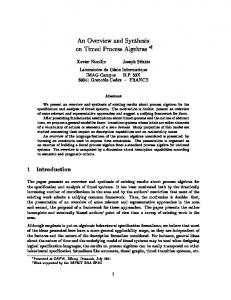
1.1 Single-task vs multi-task implementations If the original synchronous program is multi-rate, that is, contains parts that execute at different periods or are triggered by different events, then the single-task implementation must run at the fastest possible rate. Inside the code, if-then statements can be used to execute the parts that run at slower rates. This presents no problems as long as the monolithic program can be executed fast enough, that is, as long as its worst-case execution time (WCET) is smaller than the activation period (or minimum inter-arrival time of triggering events, in case the program is aperiodic). If this condition fails, however, then the monolithic implementation may fail to react promptly or may even miss triggering events. For example, consider a synchronous program consisting of two parts (or tasks) P1 and P2 that must be executed every 10 and 100 ms, respectively. Suppose the worst-case execution time (WCET) of P1 and P2 is 2 and 10 ms, respectively, as shown in Figure 1. Then, in a monolithic implementation, a single task P that includes the code of both P1 and P2 would have to be executed every 10 ms, since this is required by P1 . Inside P , P2 would be executed only once every 10 times (e.g., using an internal counter modulo 10). Assuming that the WCET of P is the sum of the WCETs of P1 and P2 (note that this might not always the case), we find that the WCET of P is 12 ms, that is, greater than its period. In practice, this means that every ten times, the task P1 will be delayed by 2 ms. This may appear harmless in this simple case, but the delays might be larger and much less predictable in more complicated cases. This obviously has an effect on semantical preservation: the outputs produced by the single-task implementation may be different from those defined by the synchronous semantics. Until recently, there has been no rigorous methodology for handling this problem. In the absence of such a methodology, industrial practice consists in “manually” modifying the synchronous design, for instance, by “splitting” tasks with large execution times, like task P2 above. Clearly, this is not satisfactory as it is both tedious and error-prone. Multi-task implementations can provide a remedy to schedulability problems as the one discussed above. When an RTOS is available, and the two tasks P1 and P2 do not communicate with each other (i.e., do not exchange data in the original synchronous design), there is an obvious solution: generate code for two separate tasks, and let the RTOS handle the scheduling of the two tasks. Depending on the scheduling policy used, some parameters need to be defined. For instance, if the RTOS uses a static-scheduling policy, as this is the case most of the times, then a priority must be assigned to each task prior to execution. During execution, the highest-priority task among the tasks that are ready to execute is chosen. In the case of multi-periodic tasks, as in the example above, the rate-monotonic assignment ACM Transactions on Embedded Computing Systems, Vol. V, No. N, July 2007.

4

·

Paul Caspi et al

policy is known to be optimal in the sense of schedulability [Liu and Layland 1973]. This policy consists in assigning the highest priority to the task with the highest rate (i.e., smallest period), the second highest priority to the task with the second highest rate, and so on. This solution is simple and works correctly as long as the tasks do not communicate with each other. However, this is not a common case in practice. Typically, there will be data exchange between tasks of different periods. In such a case, some inter-task communication mechanism must be used. On a single processor, this mechanism usually involves some form of buffering, that is, shared memory accessed by one or more tasks. Different buffering mechanisms exist: —simple ones, such as a buffer for each pair of writer/reader tasks, equipped with a locking mechanism to avoid corruption of data because of simultaneous reads and writes. —same as above but also equipped with a more sophisticated protocol, such as a priority inheritance protocol to avoid the phenomenon of priority inversion [Sha et al. 1990], or a lock-free protocol to avoid blocking upon reads or writes [Chen and Burns 1997; Huang et al. 2002]. —other shared-memory schemes, like the publish-subscribe scheme used in the PATH project [Puri and Varaiya 1995; Tripakis 2002], which allows decoupling of writers and readers. None of these buffering schemes, however, guarantees preservation of the original synchronous semantics 4 . This means that the sequence of outputs produced by some task at the implementation may not be the same as the sequence of outputs produced by the same task at the original synchronous program. Small discrepancies between semantics and implementation can sometimes be tolerated, for instance, when the task implements a robust controller which has built-in mechanisms to compensate for errors. In other applications, however, such discrepancies may result in totally wrong results, with catastrophic consequences. For example, controllers contain more and more ”discrete logic”, which is not robust (a single bit-flip may change the course of an if-then-else statement). Moreover, echos from the industry indicate that determinism is an important requirement. For instance, recent versions of the Simulink code-generator Real-Time Workshop provide options to ”ensure deterministic data transfer”. Our contacts with Esterel Technologies reveal similar concerns. Having a method that guarantees equivalence of semantics and implementation is then crucial. It implies that the effort spent in simulation or verification of the synchronous program need not be duplicated in order to test the implementation, which is an extremely important cost factor. 1.2 Contributions In this paper we propose a set of semantics-preserving, multi-task implementation techniques for synchronous programs. We model synchronous programs abstractly, 4 Many of these schemes guarantee a freshest-value semantics, where the reader always gets the latest value produced by the writer (in Section 3.3 we provide such an example of non preservation of the synchronous semantics). Freshness is desirable in some cases, in particular in control applications, where the more recent the data, the more accurate they are.


Semantics-Preserving Multi-Task Implementation of Synchronous Programs

·

5

as sets of communicating tasks. Tasks are triggered by different events and we make no assumption on the occurrence pattern of these events. The synchrony hypothesis is captured in the semantics of the model, which is “ideal”: a task produces its output as soon as it is triggered, that is, in zero time. We then define a set of inter-task communication schemes, each of which involves a set of buffers shared by writer and reader tasks, a set of pointers pointing to these buffers and a protocol to manipulate buffers and pointers. The essential principle behind all protocols is that the pointers must be manipulated not during the execution of the tasks, but upon the arrival of the events triggering these tasks. In that way, the order of arrivals can be “memorized” and the original semantics can be preserved. In Section 3.3 we provide a concrete example in which the above principle is not implemented and as a result the ideal semantics is not preserved. More precisely, we propose two types of buffering protocols: static and dynamic. In the static buffering protocols, the set of buffers is determined before execution. These protocols are more efficient time-wise, however, they are generally non-optimal with respect to memory requirements, when the writer communicates data to more than one reader. For this reason, we also propose a dynamic buffering protocol, called DBP, which allocates buffers only when they are needed, at the expense of some time overhead. The protocols can be applied when the tasks are scheduled using one of the following two types of preemptive scheduling policies: static-priority (SP) scheduling or earliest-deadline first (EDF) scheduling [Liu and Layland 1973]. Note also that the static protocols are in fact special cases of the DBP. Each static buffering protocol involves a writer task τi and a reader task τj . There are three protocols, depending on the relative priorities of τi and τj , in case SP scheduling is used, or their relative deadlines, in case EDF scheduling is used. —The high-to-low protocol is used when τi has higher priority than τj , or smaller deadline. —The high-to-low protocol with unit-delay is used when τi has higher priority than τj , or smaller deadline, and there is a unit-delay between the two tasks, that is, τj reads the one-before-last value written by τi . —The low-to-high protocol is used when τi has lower priority than τj , or larger deadline, and there is a unit-delay between the two tasks. Notice that there is no protocol to handle the low-to-high case without unitdelay. Indeed, in this case it is impossible to preserve the zero-time semantics, as mentioned above and as explained in Section 3.3. What is also interesting to note is that, although under SP the protocols are different depending on the relative priorities of the tasks, and despite the fact that under EDF priorities change dynamically, the protocols for EDF are chosen statically, simply by considering the relative deadlines of tasks. For example, when τi has smaller deadline than τj then the high-to-low protocol is used. It turns out that even in situations where τi does not preempt τj (this is possible under EDF whereas it would preempt it under SP) the protocol works correctly. The DBP buffering protocol involves one writer task communicating the same set of data to many reader tasks. Some readers may be of higher-priority (or smallerdeadline) and some of lower-priority (or larger-deadline). Some readers may involve ACM Transactions on Embedded Computing Systems, Vol. V, No. N, July 2007.

6

·

Paul Caspi et al

a unit-delay while others do not. DBP allocates buffers upon arrivals of the writer task, whenever this is necessary, that is, when all previously allocated buffers are still in use. As we show in this paper, DBP is optimal in terms of number of buffers used. In particular, DBP uses n + 1 buffers for n lower-priority readers. This is to be compared with 2n buffers used by the static protocol. When there are also higher-priority readers, the requirements are n + 2, which is independent of the number of higher-priority readers. It should be emphasized that all protocols work no matter what the arrival pattern of tasks is. In particular, they work for both time-triggered (e.g., multi-periodic) and event-triggered applications. In the case where the arrival pattern of tasks is known a-priori, DBP can be easily turned into a static protocol, as we show in Section 5.3. 2. AN INTER-TASK COMMUNICATION MODEL We consider a set of tasks, T = {τ1 , τ2 , ...}. The set need not be finite, which allows the modeling of, for example, dynamic creation of tasks. To model inter-task communication, we consider a set of data-flow links of the form (i, j, p), with i, j ∈ {1, 2, ...} and p ∈ {−1, 0}. If p = 0 then we write τi → τj , −1

otherwise, we write τi → τj . The tasks and links result in what we shall call a task graph. For each i, j pair, there can only be one link, so we cannot have both τ i → τj −1

and τi → τj . Intuitively, a link (i, j, p) means that task τj receives data from task τi . If p = 0 then τj receives the last value produced by τi , otherwise, it receives the one-beforelast value (i.e., there is a “unit delay” in the link from τi to τj ). In both cases, it is possible that the first time that τj occurs5 there is no value available from τi (either because τi has not occurred yet, or because it has occurred only once and p = −1). To cover such cases, we will assume that for each task τi there is a default output value y0i . Then, in cases such as the above, τj uses this default value. Notice that links model data-flow, and not precedences between tasks. We allow for cycles in the graph of links, provided these cycles are not zero-delay, that is, provided there is at least one link (i, j, −1) in every cycle. Notice that we could allow zero-delay cycles if we made an assumption on the arrival patterns of tasks, namely, that all tasks in a zero-delay cycle cannot occur at the same time. However, it is often the case that tasks occur at the same time. For instance, two periodic tasks with the same initial phase, will “meet” at multiples of the least common multiplier of their periods. Synchronous, zero-time semantics We associate with this model an “ideal”, zero-time semantics. For each task τ i we associate a set of occurrence times Ti = {ti1 , ti2 , ...}, where tik ∈ R≥0 and tik < tik+1 for all k. Because of the zero-time assumption, the occurrence time captures the release, start and finish times of a task. The release time refers to the time the task becomes ready for execution. The start time refers to the time the task starts 5 As we shall see shortly, we define an “ideal” zero-time semantics where a task executes and produces its result as the same time it is released. We can thus say “task τ i occurs”.



·

7

execution. The end time refers to the time the task finishes execution. In the next section, we will distinguish these three times. We make no assumption on the occurrence times of a task. This allows us to capture all possible situations, namely, where a task is periodic (i.e., released at multiples of a given period) or where a task is aperiodic or sporadic. Also note that for two tasks i and j, we might have tik = tjm , which means that i and j may occur at the same time. The absence of zero-delay cycles ensures that the semantics will still be well-defined in such a case. Given time t ≥ 0, we define ni (t) to be the number of times that τi has occurred until t, that is: ni (t) = |{t0 ∈ Ti | t0 ≤ t}|. We denote inputs of tasks by x’s and outputs by y’s. Let yki denote the output of the k-th occurrence of τi . Given a link τi → τj , xi,j k denotes the input that the k-th occurrence of τj receives from τi . The ideal semantics specifies that this input is equal to the output of the last occurrence of τi before τj , that is: j i xi,j k = y` , where ` = ni (tk ).

Notice that if τi has not occurred yet then ` = 0 and the default value y0i is used. −1 If the link has a unit delay, that is, τi → τj , then: j i xi,j k = y` , where ` = max{0, ni (tk ) − 1}.

Some examples of the ideal semantics are provided in the next section, where we also show potential problems that arise during implementation. 3. EXECUTION ON STATIC-PRIORITY OR EDF SCHEDULERS 3.1 Execution under preemptive scheduling policies We consider the situation where tasks are implemented as stand-alone processes executing on a single processor equipped with a real-time operating system (RTOS). The RTOS implements a scheduling policy to determine which of the ready tasks (i.e., tasks released but not yet completed) is to be executed at a given point in time. In this paper, we consider two scheduling policies: —Static-priority: each task τi is assigned a unique priority pi . The task with the highest (greatest) priority among the ready tasks executes. We assume no two tasks have the same priority, that is, i 6= j ⇒ pi 6= pj . This implies that at any given time, there is a unique task that may be executed. In other words, the scheduling policy is deterministic, in the sense that for a given pattern of release and execution times, there is a unique behavior. —Earliest-deadline first or EDF: each task is assigned a unique (relative) deadline (in short, deadline). We assume no two tasks have the same deadline, that is, i 6= j ⇒ di 6= dj . The task with the smallest absolute deadline among the ready tasks executes. The absolute deadline of a task is equal to r + d, where r is the release time of the task and d is the deadline. In the ideal semantics, task execution takes zero time. In reality, this is not true. A task is released and becomes ready. At some later point it is chosen by the ACM Transactions on Embedded Computing Systems, Vol. V, No. N, July 2007.

8

·

Paul Caspi et al

scheduler to execute. Until it completes execution, it may be preempted a number of times by other tasks. To capture this, we distinguish, as explained above, the release time of a task τi from the time τi begins execution and from the time τi ends execution. For the k-th occurrence of τi , these three times will be denoted rki , bik and eik , respectively. Throughout this work, we make only one assumption concerning the release times of the different tasks, namely, that the tasks are schedulable. Schedulability means that no task ever violates its absolute deadline, that is, that the release of a task cannot be prior to the completion of the previous instance, if there exists any, of the same task. Therefore, in the static-priority case, we assume that the absolute deadline is the next release time of the task, that is, the absolute deadline of the i k-th occurrence of τi is rk+1 . In the EDF case, if di is the deadline of τi , then the absolute deadline of the k-th occurrence of τi is rki + di . Obviously, schedulability depends on the assumptions made on the release times and execution times of tasks. Checking schedulability is beyond the scope of this work. A large amount of work exists on schedulability analysis techniques for different sets of assumptions: see, for instance, the seminal paper of Liu and Layland [Liu and Layland 1973], the books [Harbour et al. 1993; Stankovic et al. 1998], or more recent schedulability methods based on timed automata model-checking [Fersman and Yi 2004]. Notice, however, that our assumption of schedulability is not related to a specific schedulability analysis method: it cannot be, since we make no assumptions on release times and execution times of tasks. 3.2 A “simple” implementation Our purpose is to implement the set of tasks so that the ideal semantics are preserved by the implementation. It is worth examining a few examples in order to see that a “simple” implementation does not preserve the ideal semantics. What we call simple implementation is a buffering scheme where, for each link τi → τj , there is a buffer Bi,j used to store the data produced by τi and consumed by τj . This buffer must ensure data integrity: a task writing on the buffer might be preempted before it finishes writing, leaving the buffer in an inconsistent state. To avoid this, we will assume that the simple implementation scheme uses atomic reads and writes, so that a task writing to or reading from a buffer cannot be preempted before finishing. −1 For links with unit delays, of the form τi → τj , the simple implementation scheme 1 1 0 uses a double buffer (Bi,j , Bi,j ). Bi,j is used to store the current value written by the producer (i.e., the value written by the last occurrence of the producer) and 0 is used to store the previous value (i.e., the value written by the one-before-last Bi,j occurrence). Every time a write occurs, the data in the buffers is shifted, that is, 0 1 1 Bi,j is set to Bi,j and Bi,j is overwritten with the new value. The reader always 0 reads from Bi,j . Reads and writes are again atomic. For the purposes of this section, we assume that each task is implemented in a way such that all reads happen right after the beginning and all writes happen right before the end of the execution of the task. Also, there is only one read/write per pair of tasks, that is, if τi → τj then τi cannot write twice to τj . These assumptions are not part of the implementation scheme. They are a “programming ACM Transactions on Embedded Computing Systems, Vol. V, No. N, July 2007.

·


9

style”. Our aim is to show that, even when this programming style is enforced, the ideal semantics are not generally preserved. Note that these assumptions are not needed in the sections that follow: the protocols we propose work even when these assumptions do not hold. However, we will assume that every writer task writes at least once at each occurrence. This is not a restrictive assumption since “skipping” a write amounts to memorizing the previously written value (or the default output) and writing this value. 3.3 Problems with the “simple” implementation Even with the above provisions, the ideal semantics are not always preserved. Consider, as a first example, the case τi → τj , where static-priority scheduling is used and τi has lower priority than τj , pi < pj . Consider the situation shown in Figure 2. We can see that, according to the semantics, the input of the m-th occurrence of τj is equal to the output of the (k + 1)-th occurrence of τi . However, this is not true in the implementation, because τj preempts τi before the latter has time to finish, thus, before it has time to write its result.

j rm i xjm = yk+1

i rk+1 i yk+1

rki yki

a: ideal semantics

τi rki

τj

τi yki

i rk+1

j rm j xm =

τi i yk+1

yki

b: simple implementation i Fig. 2. In the semantics, xjm = yk+1 , whereas in the implementation, xjm = yki .

One possible solution to the above problem is to use some type of priorityinheritance protocol, which essentially “lifts” the priority of a task while this task is accessing a resource: see, for instance [Sha et al. 1990]. In such protocols, the consumer task “blocks” and waits for the producer task to finish. In this work, we are interested in wait-free solutions because they are easier to implement. However, there is no wait-free solution to the above problem, unless we require that, whenever τi has lower priority than τj and τj receives data from τi , a unit delay is used between ACM Transactions on Embedded Computing Systems, Vol. V, No. N, July 2007.

·

10

Paul Caspi et al −1

the two tasks, in other words, the link must be: τi → τj . From now on, we will assume that this is the case. Even when the above requirement is satisfied, the simple implementation scheme −1 is not correct. Consider the case τi → τj , where pi < pj , that is, a low-to-high priority communication, with unit delay. Suppose there is another task τq with pq > pj > pi . Consider the situation shown in Figure 3, where the order of task releases is τi , τi , τq , τi and τj . In the ideal semantics, the reader task τj uses the i i output yk−1 . However, in the simple implementation, it uses the output yk−2 . This is because τq “masks” the releases of τi and τj , which results in an execution order of τi and τj which is the opposite of their arrival order.

rlq

i rk−1 i yk−1

i rk−2 i yk−2

rki yki

j rm i xjm = yk−1

a: ideal semantics

τq τi i rk−2

τj

τi i yk−2

i rk−1

i yk−1

rlq

rki

j rm

τi

i xjm = yk−2

b: simple implementation i i Fig. 3. In the semantics, xjm = yk−1 , whereas in the implementation, xjm = yk−2 .

As a third example, consider the high-to-low static-priority case, where the producer has higher priority than the consumer. In particular, we have τi → τj and pi > pj . There is also a third task τq with higher priority than both τi and τj , pq > pi > pj . Consider the situation shown in Figure 4. We can see that, according to the semantics, the input of the m-th occurrence of τj is equal to the output of the k-th occurrence of τi . However, this is not true in the implementation. This j i is again because τq “masks” the order of arrival of τj and τi (rm < rk+1 ). As a result, the order of execution of τj and τi is reversed and the reader τj consumes a “future” (according to the semantics) output of the writer τi . These examples show that a simple implementation scheme like the one above will fail to respect the ideal semantics. Note that the problems are not particular to static-priority scheduling. Similar situations can happen with EDF scheduling, depending on the deadlines of the tasks. For instance, the situation shown in ACM Transactions on Embedded Computing Systems, Vol. V, No. N, July 2007.


rlq

rki yki

j rm xjm = yki

·

11

i rk+1 i yk+1

a: ideal semantics

τq

τi rki

yki

rlq

j rm

τi i rk+1

τj i yk+1 xjm =

i yk+1

b: simple implementation i Fig. 4. In the semantics, xjm = yki , whereas in the implementation, xjm = yk+1 .

j i Figure 2 can occur under EDF scheduling if rm + dj < rk+1 + di . The situation q i j shown in Figure 4 can occur under EDF scheduling if rl + dq < rk+1 + di < rm + dj .

4. SEMANTICS-PRESERVING IMPLEMENTATION: THE ONE-READER CASE To overcome the above problems, we propose an implementation scheme that preserves the ideal semantics. The scheme can be applied to both cases of static-priority and EDF scheduling. For simplicity and in order to facilitate understanding, we first present the scheme in the special case of a writer task communicating to a single reader task. In this case, there are three protocols depending on the relative priorities (or deadlines) of the tasks as well as on whether a unit-delay is present or not. Thus, there are three protocols: the low-to-high protocol, the high-to-low protocol and the high-to-low protocol with unit-delay. These protocols are special cases of the general protocol presented in Section 5. The first is used in the static-priority case when the writer task has lower priority than the reader task, or in the EDF case when the writer has smaller deadline than the reader. The second is used in the static-priority case when the writer has higher priority than the reader, or in the EDF case when the writer has greater deadline than the reader. The third is used in the same cases as the second, but where there is a unit-delay between the writer and the reader. The essential idea of all protocols is that, contrary to the simple implementation scheme of the previous section, actions must be taken not only while tasks execute but also when they are released. These actions are simple (and inexpensive) pointer manipulations. They can therefore be provided as operating system support. The protocols specify such release actions for both writer and reader tasks. It is essential for the correctness of the protocol that when both writer and reader tasks are released simultaneously, writer release actions are performed before reader release actions. ACM Transactions on Embedded Computing Systems, Vol. V, No. N, July 2007.

greater smaller

12

·

Paul Caspi et al

4.1 The low-to-high buffering protocol The low-to-high buffering protocol is described in Figure 5. Notice that, as mentioned in the previous section, we assume a unit-delay between writer and reader. In this protocol, the writer τi maintains a double buffer and a one-bit variable current. The reader τj maintains a one-bit variable previous. current points to the buffer currently written by τi and previous points to the buffer written by the previous occurrence of τi . The buffers are initialized to the default value y0i and current is initialized to 0. previous does not need to be initialized, since it is set by the reader task upon its release. When the writer task is released, it toggles the current bit. When the reader task is released, it copies the negation of the current bit and stores it in its local variable previous. Notice that these two operations happen when the tasks are released, and not when the tasks start executing. During execution, the writer writes to B[current] and the reader reads from B[previous]. A typical execution scenario is illustrated in Figure 6. We assume static-priority scheduling in this example. One time axis is shown for each task. The double buffer is shown in the middle. The arrows indicate where each task writes to or reads from. In this example, the low-priority writer is preempted by the high-priority reader. It is worth noting that the beginning of execution of the high-priority task does not always coincide with its release. This is because, in general, there may be other tasks with even higher priority and they may delay the beginning of the task in question (in fact, they may also preempt it, but this is not shown in the figure). It can be checked that the semantics are preserved. A proof of preservation is provided in Section 6. 4.2 The high-to-low buffering protocol The high-to-low buffering protocol is described in Figure 7. In this protocol, it is the reader τj that maintains a double buffer. The reader also maintains two one-bit variables current, next. current points to the buffer currently being read by τ j and next points to the buffer that the writer must use when it arrives next, in case it preempts the reader. The two buffers are initialized to the default value y0i and both bits are initialized to 0. When the reader task is released, it copies next into current, and during its execution, it reads from B[current]. When the writer task is released, it checks whether current is equal to next. If they are equal, then a reader might still be reading from B[current], therefore, the writer must write to the other buffer, in order not to corrupt this value. Thus, the writer toggles the next bit in this case. If current and next are not equal, then this means that one or more instances of the writer have been released before any reader was released, thus, the same buffer can be re-used. During execution, the writer writes to B[next]. A typical execution scenario is illustrated in Figure 8. This example also assumes static-priority scheduling. Here, it is the reader that is preempted. It is worth noting that the beginning of execution of the high-priority writer does not coincide with its release. This is because, in general, there may be other tasks with even higher priority and they may delay the beginning of the writer. In fact, such tasks may also preempt the writer, but this is not shown in the figure. ACM Transactions on Embedded Computing Systems, Vol. V, No. N, July 2007.


·

13

−1

Communication: τi → τj . Task τi maintains a double buffer B[0,1] and a one-bit variable current. Task τj maintains a bit previous. Initially, current = 0 and B[0] = B[1] = y0i . During execution: —When —While —When —While

τi τi τj τj

is released: current := not current. executes it writes to B[current]. is released: previous := not current. executes it reads from B[previous].

Applicable under static-priority scheduling when pi < pj . Applicable under EDF scheduling when di > dj .

Fig. 5.

Low-to-high buffering protocol.

High

rkj

j rk+1

j rk+2

Low preemption

i rm

i rm+1 Fig. 6.

i rm+2 A typical low-to-high communication scenario.

4.3 The high-to-low buffering protocol with unit-delay −1

This protocol is intended for the case τi → τj . Before presenting this protocol, we must first point out that we can often handle this case without need for a new protocol, but using the high-to-low protocol presented above. This can be done by modifying the writer task τi so that it outputs not only its usual output y i but also the previous value of y i . That is, the k-th occurrence of τi will output both yki and i yk−1 , for k = 1, 2, .... This can be done at the expense of adding an internal buffer to τi , which stores the previous value of the output. Then, it suffices to “connect” −1 i the reader τj to yk−1 , which means that we have transformed the link τi → τj into a link τi → τj . Thus, we can use the high-to-low protocol of Section 4.2. The modification of τi suggested above is not always possible, since it requires ACM Transactions on Embedded Computing Systems, Vol. V, No. N, July 2007.

14

·

Paul Caspi et al Communication: τi → τj . Task τj maintains a double buffer B[0,1] and two one-bit variables current, next. Initially, current = next = 0 and B[0] = B[1] = y0i . During execution: —When —While —When —While

τi τi τj τj

is released: if current = next, then next := not next. executes it writes to B[next]. is released: current := next. executes it reads from B[current].

Applicable under static-priority scheduling when pi > pj . Applicable under EDF scheduling when di < dj .

Fig. 7.

High-to-low buffering protocol.

High

i rk+2

i rk+1

rki

Low

preemption

j rm+1

j rm Fig. 8.

A typical high-to-low communication scenario.

access to the task internals (e.g., source code). This is not always available, for instance, because of intellectual property restrictions. For this reason, we also provide a protocol dedicated to the high-to-low with unit-delay case. This protocol can be used by considering the writer and reader tasks as “black boxes”. The high-to-low buffering protocol with unit-delay is described in Figure 9. In this protocol, the reader τj maintains a triple buffer. There are also three pointers previous, current and reading. previous points to the buffer that contains the previous last value written by τi . This is the value that was written by the execution of the one before last occurrence of the writer (the execution that correspond to the previous last release of the writer). current points to the buffer that the writer last wrote to or is still writing to. Finally, reading points to the buffer that τ j is ACM Transactions on Embedded Computing Systems, Vol. V, No. N, July 2007.


·

15

reading from. Buffer B[0] is initialized to the default value y0i . Pointers previous and reading are initialized to 0 whereas current is initialized to 1. 0. When the reader task is released, it copies previous into reading, and during its execution reads from B[reading]. When the writer is released, it sets previous to current, so that previous points to the value previously written. Then, current is assigned to a free position in the buffer, that is, a position different from both previous and reading. Note that after the first execution the previous pointer will still point in the first buffer which has the default value.

−1

Communication: τi → τj . Task τj maintains a triple buffer B[0..2] and three one-bit variables previous, current, reading. Initially, previous = reading = current = 0, B[0] = y 0i . During execution: —When τi is released: previous := current; current := x∈[0..2].(x 6= previous ∧ x 6= reading). —While τi executes it writes to B[current]. —When τj is released: reading := previous. —While τj executes it reads from B[reading].

Fig. 9.

High-to-low buffering protocol with unit delay.

High rin+1

rin

rin+2

preemption

Low rjm Fig. 10.

rjm+1

A typical high-to-low with unit delay communication scenario.


16

·

Paul Caspi et al

Small deadline

j

rk

j

j

rk+2

rk+1

Large deadline

i rm

i rm+1

Fig. 11.

i rm+2

The scenario of Figure 6 possibly under EDF: τi is not preempted.

4.4 Some examples under EDF scheduling All examples we have given so far have assumed static-priority scheduling. In this section, we provide some informal arguments and examples to justify intuitively why the protocols can also be applied to EDF. Notice that, a priori, one might think that the protocols are not applicable to EDF, for the following reason. Under EDF, the priorities of tasks change dynamically. On the other hand, the above protocols have been designed assuming a static priority assignment to the writer and the reader. Indeed, if the two priorities are swapped, a different protocol must be used. These facts could lead one to conclude that, under EDF, the buffering scheme needs to be dynamic as well. Fortunately, this is not the case: the buffering scheme can be defined statically, that is, before execution begins. In particular, the buffering scheme depends on the relative deadlines di and dj of the writer τi and the reader τj , respectively. —If di > dj then the low-to-high buffering scheme is used. Again, we assume a unit-delay between τi and τj , in order to avoid the problem of Figure 2. —If di < dj and τi → τj , then the high-to-low buffering scheme is used. −1

—If di < dj and τi → τj , then the high-to-low with unit-delay scheme is used. The case di > dj implies that, if τj is released before τi then τi cannot preempt i τj , neither can it start before τi ends. Indeed, rkj ≤ rm and dj < di implies j i rk + d j < r m + di , that is, the absolute deadline of τj is smaller than that of τi . Therefore, we have a situation which is “almost the same” as the low-to-high staticpriority case. The difference is that in the static-priority case τj always preempts τi , whereas in the EDF case this might not happen. Therefore, in order to guarantee the correctness of the scheme, we must examine this last possibility, to ensure that nothing goes wrong. Figure 11 illustrates what might happen when τj does not preempt τi as it normally would in the low-to-high static-priority scenario. One can see that this poses no problems for the buffering scheme. In fact, the situation is as if the k-th instance ACM Transactions on Embedded Computing Systems, Vol. V, No. N, July 2007.


·

17

of τj was released after the (m + 1)-th instance of τi finished. Let us now turn to the case di < dj . This case implies that, if τi is released before j τj then τj cannot preempt τi , neither can it start before τi ends. Indeed, rki ≤ rm i j and di < dj implies rk + di < rm + dj , that is, the absolute deadline of τi is smaller than that of τj . Therefore, we have a situation which is “almost the same” as the high-to-low priority case. The difference is that in the high-to-low priority case τ i always preempts τj , whereas in the EDF case this might not happen. As before, we must examine this possibility. Figure 12 illustrates what might happen when τi does not preempt τj as it normally would in the high-to-low static-priority scenario. Again, this poses no problems to the buffering scheme. The situation is as if the (k + 1)-th instance of τi was released after the m-th instance of τj finished.

Small deadline

i rk

i rk+1

i rk+2

Large deadline

j

j rm

Fig. 12.

rm+1 The scenario of Figure 8 possibly under EDF: τj is not preempted.

−1

The same situation is for the case where τi → τj and di < dj . Figure 13 shows a typical execution, where the writer task does not preempt the reader, despite the fact that the latter has larger deadline. This does not cause any problem, however. In fact, the situation is exactly the same as the one where τi arrives after τj finishes. It is worth noting that, contrary to static-priority scheduling, under EDF scheduling, there are cases where the choice of which task to execute next is non-deterministic. This is when the absolute deadlines of two tasks are equal6 . Such non-determinism in scheduling is not problematic for our protocol. 6 Note that the assumption we made in Section 3 that relative deadlines of two tasks are different does not guarantee that their absolute deadlines will also be different. On the other hand, the assumption that the static priorities of tasks are different suffices to guarantee deterministic static priority scheduling.


18

·

Paul Caspi et al

Small deadline

rin+1

rin

rin+2

Large deadline rjm Fig. 13.

rjm+1

The scenario of Figure 10 possibly under EDF: τj is not preempted.

4.5 Application to general task graphs The three protocols presented above can also be used in a general task graph as the one described in Section 2. Here, we show how this can be done in a simple way. Notice that the method we present here is not always optimal in terms of buffer utilization. Section 5 presents a generalized protocol which is also optimal. We can assume that tasks are ordered with respect to their priorities or deadlines, depending on whether we are in a static-priority or EDF setting, respectively. For instance, in a static-priority setting, we assume that tasks are ordered as τ 1 , τ2 , ..., meaning that τ1 has the highest priority, τ2 has the second highest, and so on. In an EDF setting, τ1 has the smallest deadline, and so on. We will also assume, as we already said above, that there is no link τi → τj such that i > j. This would correspond to the low-to-high priority case without unit-delay, where semantics cannot be generally preserved. Thus, with i > j, we −1 −1 have only three types of links, namely, τi → τj , τj → τi and τj → τi . One simple way of using the protocols is to consider each data-flow link separately. −1 In other words, assuming i > j, for each link τi → τj we apply the low-to-high protocol, for each link τj → τi we apply the high-to-low protocol, and for each link −1 τj → τi we apply the high-to-low protocol with unit-delay. This method results in a memory requirement of 2M + 2N1 + 3N2 (single) buffers, where M is the number −1 of τi → τj links in the task graph, N! is the number of τj → τi links and N2 is −1

the number of τj → τi links. We also have memory requirements for the one-bit variables, but these are negligible. Note that we use the notation of M ,N1 and N2 because it will be similar (corresponding to the case we use) when we explain the generalized protocol in Section 5.1. We can immediately improve the above memory requirement by observing that, in the case of the low-to-high protocol, it is the writer that maintains the double ACM Transactions on Embedded Computing Systems, Vol. V, No. N, July 2007.

·


19

−1

buffer and not the reader. Therefore, if we have a set of links τi → τjk with i > jk for k = 1, ..., M , and if τi communicates the same data to all tasks τjk , then we do not need 2m buffers, but only 2. Let us give an example. Consider the task graph shown in Figure 14. Unit-delays are depicted as −1 on the links. Notice that all unit-delays are mandatory, except −1 the one on the link τ3 → τ4 . We assume that every writer communicates the same data to all readers. Using the simple method, we have buffer requirements equal to 2M +2N1 +3N2 = 2 ∗ 4 + 2 ∗ 2 + 3 ∗ 1 = 15. Using the improved method, the buffers maintained by each task are as follows: —τ1 is the highest-priority (or lowest-deadline) task. It maintains one double buffer as the writer of the link τ1 → τ3 . It maintains no buffer as a reader, since in this case the buffers are maintained by the lower-priority writers. —τ2 maintains no buffer. −1

−1

—τ3 maintains one double buffer as the writer of the links τ3 → τ1 and τ3 → τ2 . −1

−1

—τ4 maintains one double buffer as the writer of the links τ4 → τ1 and τ4 → τ2 . −1 τ4 also maintains a triple buffer as the reader of the link τ3 → τ4 . —τ5 maintains one double buffer as the reader of the link τ3 → τ5 . Thus, in total, the improved method uses 2 + 2 + 2 + 3 + 2 = 11 buffers, or 4 buffers less than the simple method. There is still room for improvement, however. In particular, we show in the next section how the buffer requirements can be optimized. −1

τ2

τ3

−1

τ4 −1 −1

τ1 τ5 −1

Fig. 14.

A task graph.

5. SEMANTICS-PRESERVING IMPLEMENTATION: THE GENERAL CASE As already mentioned, the protocols presented in Section 4 are specializations of a generalized protocol, called DBP, that we present in this section. DBP is used for one writer communicating (the same) data to N lower-priority (or larger-deadline) ACM Transactions on Embedded Computing Systems, Vol. V, No. N, July 2007.

20

·

Paul Caspi et al M higher-priority readers with unit delay −1 writer −1

N2 lower-priority readers with unit-delay

N1 lower-priority readers

Fig. 15.

Applicability of the DBP protocol.

readers and M higher-priority (or smaller-deadline) readers, as shown in Figure 15. In N1 among the N lower-priority readers there is no unit-delay, while in the rest N2 = N − N1 readers there is a unit-delay. DBP can be applied to general (i.e., multi-writer) task graphs as we show in Section 5.2. Apart from being semantics-preserving, DBP also allows to reduce the memory requirements with respect to the simple method presented in Section 4.5. In particular, DBP requires N + 2 (single) buffers, assuming M 6= 0 and N2 6= 0. If M = N2 = 0 (i.e., there are no readers linked with a unit-delay) then DBP requires N +1 = N1 +1 buffers. This is to be compared, for example, to 2N buffers required when using the method of Section 4.5. Buffer requirements are presented in detail in Section 7. 5.1 The Dynamic Buffering Protocol DBP is shown in Figure 16. The figure shows the protocol in the case where M 6= 0 or N2 6= 0, that is, the case where there are links with unit-delay. If M = N2 = 0 then the protocol is actually simpler: the pointer previous is not needed and instead of N + 2 = N1 + 2, only N1 + 1 buffers are needed. The operation of DBP is as follows. The writer τw maintains all buffers and pointers except the pointers of the higher-priority readers P[i]. The current pointer points to the position that the writer last wrote to. The previous pointer points to the position that the writer wrote to before that. R[i] points to the position that τi must read from. The key point is that when the writer is released, a free position in the buffer array must be found, and this is where the writer must write to. By free we mean a position which is not currently in use by any reader, as defined by the predicate free(j). Finding a free j ∈ [1..N + 2] amounts to finding some j which is different from previous (because B[previous] may be used by the higher-priority reader or a possible lower-priority with unit-delay reader may need to copy its value) and also different from all R[i] (because B[R[i]] is used, or will be used, by the lowerpriority reader τi ). Notice that such a j always exists, by the pigeon-hole principle: there are N + 2 possible values for j and up to N + 1 possible values for previous and all R[i]. Finding a free position is done in the second instruction executed upon the release of the writer. The first instruction updates the previous pointer. This pointer is copied by each higher-priority reader τi0 , when released, into its local variable P[i]. ACM Transactions on Embedded Computing Systems, Vol. V, No. N, July 2007.


·

21

Communication: −1 −1 τw → τi , for i = 1, ..., N1 , τw → τi , for i = N1 + 1, ..., N1 + N2 , and τw → τi0 , for i = 1, ..., M . Let N = N1 + N2 . Task τw maintains a buffer array B[1..N +2], one pointer array R[1..N ] and two pointers current and previous. Each task τi0 , for i = 1, ..., M , maintains a local pointer P[i]. All pointers are integers in [1..N +2]. A pointer can also be null. Initially, current = previous = 1, all R[i] and P[i] are set to null, and all buffer elements are set to y0i . During execution: Writer: —When τw is released: previous := current; current := some j∈[1..N +2]such that free(j), where free(j) ≡ (previous6=j ∧ ∀i∈[1..N ].R[i]6=j). —While τw executes it writes to B[current]. Lower-priority reader τi : —When τi is released: if i∈[1..N1 ] then R[i] := current else R[i] := previous —While τi executes it reads from B[R[i]]. —When τi finishes: R[i] := null.

(link τw → τi ) −1

(link τw → τi )

Higher-priority reader τi0 : —When τi0 is released: P[i] := previous. —While τi0 executes it reads from B[P[i]]. Applicable under static-priority scheduling when ∀i = 1, ..., N . pi < pw . and ∀i = 1, ..., M . p0i > pw . Applicable under EDF scheduling when ∀i = 1, ..., N . di > dw and ∀i = 1, ..., M . d0i < dw .

Fig. 16.

The protocol DBP.

τi0 then reads from B[P[i]]. When a lower-priority reader τi is released, we have two cases: (i) either τi is one of the N1 readers that are linked without a unit-delay, or (ii) τi is one of the N2 readers that are linked with unit-delay. In case (i) τi needs the last value written by the writer. In case (ii) τi needs the previous value. Pointer R[i] is set to the needed value. Besides this pointer assignment the rest of the procedure remains the same for both kinds of lower-priority readers. While executing, τi reads from B[R[i]]. When τi finishes execution, R[i] is set to null. This is done for optimization purposes, so that buffers can be re-used as early as possible. Notice that even if this operation is removed, DBP will still be correct and it will use at most N + 2 buffers. However, DBP will be sub-optimal, in the sense that the buffer pointed to by R[i] will not be freed until the next release of τi . With the above operation present, the buffer is freed earlier, namely, when the current release of τi finishes. Notice that DBP also relies on the fact that no more than one instance of every ACM Transactions on Embedded Computing Systems, Vol. V, No. N, July 2007.

22

·

Paul Caspi et al

τw

τ2

τ3 −1

τ1

Fig. 17.

Tw = 2 T1 = 1 T2 = 3 T3 = 5

A task graph with one writer and three readers.

task can be active at any point in time, which follows from the schedulability assumption. In more detail, there can be no more than one pointer per lowerpriority task, which allow us to use the pigeon hole principle as we did before. Like the protocols discussed in the previous section, DBP also specifies release actions for both writer and reader tasks. In case of simultaneous release of more than one tasks, we require that the release actions of the writer task are performed before the release actions of the simultaneously released readers. The actions of the readers can be performed in any order. Another major contribution of the above algorithm is that it does not take into account any possible initial offset of the concerning tasks. This is important mostly for the multi-periodic application of the algorithm, as we’ll study in Section 5.3, since methods used up to now, exclude the use of the initial offset. An example. To illustrate how DBP works, we provide an example. Consider the task graph shown in Figure 17. There are four tasks: one writer τw with period Tw = 2, one higher-priority reader τ1 with period T1 = 1 and two lower-priority readers τ2 and τ3 with periods T2 = 3 and T3 = 5 respectively. This means that for the one writer of this task graph N = 2, where N is the number of lower priority readers. Moreover there is one task with higher priority. Suppose the priorities of the tasks follow the rate-monotonic assignment policy (note that DBP does not require this, as it can work with any priority assignment): P rio1 > P riow > P rio2 > P rio3 . According to the algorithm, the writer will maintain a buffer array B, a pointer array R of size 2, and two pointers current and previous. Also, τ 1 maintains a local pointer P. Note that, since N = 2, B cannot grow larger than 4 buffers. The initial values are current=previous=1 and R[2]=R[3]=P[1]=null. A sample execution of DBP is shown in Figures 18 and 19. Figure 19 shows the values of the pointers during execution. Figure 18 shows the release, begin of execution and end of execution events for each task. Task τ1 is released at times 0, 1, 2, 3, 4, 5, task τw is released at times 0, 2, 4, and so on. We use the notation τ1 , τ10 , ... to denote different instances of the same task. Notice that a task instance may be “split” because of preemption: this is, for instance, the case of τ2 which ACM Transactions on Embedded Computing Systems, Vol. V, No. N, July 2007.

·

Semantics-Preserving Multi-Task Implementation of Synchronous Programs τw , τ 1 , τ 2 , τ 3

τ1

τ1

τw

0

B0 :

τw , τ 1

τ10

τ100 τ2

τ2

y1

1

2

1st cycle

B1 :

τw0

τ3

1

y0

τ1 , τ 2

y0

y1

1

2

B2 :

2nd cycle

τ1000

current previous P[1] R[2] R[3]

init 1 1 null null null

τ20

y2

y1

1

2

τ1 , τ 3

τ10000

τw00

τ3

3

τ3

4

B3 :

3rd cycle

Fig. 18.

Fig. 19.

τw , τ 1

τ3

2

23

y2

y1

1

2

B4 :

5

y2

y1

y3

1

2

3

4th cycle

5th cycle

The execution of the tasks.

0 2 1 1 2 2

1 2 1 1 2 2

2 1 2 2 null 2

3 1 2 2 1 2

4 3 2 1 null 2

5 3 2 1 null 3

The values of the DBP pointers during execution.

is split between the first and second cycle. The heights of the task “boxes” in the figure denote the relative priorities of the tasks. Figure 18 also shows exactly where each task reads from and writes to at any given time (dashed and solid arrows respectively). The “boxes” at the bottom of the figure correspond to the buffer array B and the values stored in each buffer: y0 is the initial (default) value, y1 is the value written by the first instance of τw , and so on. Notice that B grows to 3 buffers in this example. It can be verified that the synchronous semantics are preserved. For example, the first instance of reader 2, τ2 , reads the value produced by the first instance of the writer, which was released at the same time. The third instance of reader 1, τ100 , reads the same value: this is because a unit delay is present in this case. It is worth noting that the unique instance of reader 3 shown in the figure, although it is preempted multiple times, consistently reads the correct value, namely y1 . The fact that this instance has not terminated execution when the writer is released at time 4 is what triggers the allocation of a new buffer B[3]. Specializations. It can be easily shown that the three protocols presented in Section 4 are specializations of DBP. First, consider the low-to-high protocol (Figure 5). It can be obtained by using DBP with N = 0 and M = 1. Then, DBP uses two buffers B[1..2] and three pointers: previous, current, P[1]. In fact, previous is redundant since it always points to the buffer not pointed to by current. Thus, current corresponds to the pointer current of Figure 5 and P[1] corresponds to the pointer previous of Figure 5 (the latter is local to the reader). Next, consider the high-to-low protocol (Figure 7). It can be obtained by using ACM Transactions on Embedded Computing Systems, Vol. V, No. N, July 2007.

24

·

Paul Caspi et al

DBP with N2 = M = 0 and N1 = 1. As we said above, in this case only N1 + 1 = 2 buffers are needed and the pointer previous is useless. Thus, DBP uses two pointers current, R[1]: they correspond to pointers next and current of Figure 7, respectively. Finally, consider the high-to-low protocol with unit-delay (Figure 9). It can be obtained by using DBP with N1 = M = 0 and N2 = 1. Then, DBP uses three buffers B[1..3] and three pointers previous, current, R[1]: they correspond to pointers previous, current, reading of Figure 9, respectively. 5.2 Application of DBP to general task graphs Applying DBP to a general task graph is easy: we consider each writer task in the graph and apply DBP to this writer and all its readers. As an example, let us consider again the task graph shown in Figure 14. There are three writers in this graph, namely, τ1 , τ3 and τ4 . We assume, for each writer, that it communicates the same data to all its readers. Then, the buffer requirements are as follows: —τ1 has only one lower-priority reader without unit-delay. That is, we are in the case M = N2 = 0 and N1 = 1. As said above, in this case DBP specializes to the high-to-low protocol, which requires one double buffer. —τ3 has two higher-priority readers τ1 and τ2 (with unit-delay), one lower-priority reader τ4 without unit-delay and one lower-priority reader τ5 with unit-delay. That is, we are in the case N1 = N2 = 1 and M = 2. We apply DBP and we need N + 2 = 4 buffers. —τ4 has two higher-priority readers. That is, we are in the case N = 0 and M = 2. We apply DBP and we need 2 buffers. Thus, in total, we have 8 single buffers. This is to be compared to 11 single buffers needed using the method described in Section 4.5. In the case that we have more than one writer, as we said earlier, there is distinctive application of the DBP protocol with new memory space and pointers. Therefore, we do not need to take care about the execution of assignments implied by two different instances of DBP (we could impose for example a partial order for the readers and the writers depending on the priority of the writers of the corresponding DBP). This means that the assumption we expressed earlier, i.e. when a reader and a writer arrive simultaneously, we give priority to the actions of the writer, is sufficient in the general case, we just described. 5.3 Application of DBP to tasks with known arrival pattern DBP is a dynamic protocol in the sense that it reacts to task arrivals and assigns (or even allocates) buffers accordingly. This implies a run-time overhead, for instance, in order to search for a free buffer every time the writer is released. This cannot be avoided in the general case, since the task arrival times are not known in advance. In the case where task arrivals are known, we can turn DBP into a static protocol, using the method described in what follows. Known task arrival patterns are common: one case is the one of multi-periodic applications where each task is periodic with a known period. Other cases can be more involved, but still the designer may be able to predict with accuracy ACM Transactions on Embedded Computing Systems, Vol. V, No. N, July 2007.


·

25

the arrivals of tasks. We will not assume that the task arrivals are necessarily deterministic. For example, we may only know that a task will arrive within some interval, but not know exactly at what time. However, we will assume that the order of task arrivals is deterministic. Therefore, the task arrival intervals should not overlap. We will also assume that the task arrival pattern is ultimately periodic. This means that the pattern repeats itself forever after some point. This allows for a static representation of the pattern. Using this information, we can build a static periodic schedule which indicates, for each task and each occurrence of this task, where the task should write to or read from. This can be done by simulating DBP with the a priori known release order of the reader(s) and writer tasks. During simulation we keep track where the writer stores data and where the reader(s) read from. Those positions can be directly entered into a table that represents the static periodic schedule. The simulation is performed for the entire period of the arrival pattern. In the multiperiodic case, this is equal to the hyper-period of the tasks, that is, the least common multiplier of all periods. Notice that for large hyper-periods the table can become inaffordably large. In such a case the dynamic version of the protocol may be more advantageous, despite its time overhead. This is an instance of a standard trade-off between time versus memory savings. Knowledge about task arrivals can be also used in another, very important, way: namely, for memory optimizations. We briefly explain the idea here, and defer a detailed description to Section 7.3. DBP is a non-clairvoyant protocol: it reacts to task arrivals but does not know when future arrivals of a task will occur. This is because the protocol is general: it can be applied to any task arrival pattern. For reasons of memory optimization that will become clear in Section 7, it is worth specializing DBP for the case where the arrival pattern of tasks is known. In this case, DBP can exploit knowledge about future arrivals of tasks in order to reduce the number of buffers used, for example, by “freeing” a buffer written by the writer when it knows that no reader will ever use this value in the future. See Section 7.3 for details. 6. PROOF OF CORRECTNESS In this section we formally prove that the protocols proposed in Sections 4 and 5 are correct, that is, they preserve the ideal semantics. We will use two different proof techniques. For the one-writer/one-reader protocols of Section 4 we reduce correctness to a problem of model-checking on a finite-state model, where automatic verification techniques can be applied [Queille and Sifakis 1981; Clarke et al. 2000]. For the general protocol of Section 5 we provide a “manual” proof. Although the latter establishes the correctness of the special protocols as well, we believe that the model-checking proof technique is still worth presenting, because it can serve to establish correctness of other similar protocols in an automatic way. Moreover, from a historical point of view, the one-writer to one-reader protocols, have been founded earlier and the model-checking proof was used in the first place. 6.1 Proof of correctness using model-checking In order to use model-checking, we must justify why finite-state models suffice. We do this in a series of steps. ACM Transactions on Embedded Computing Systems, Vol. V, No. N, July 2007.

26

·

Paul Caspi et al

The first step is to prove correctness of each protocol for a single writer and a single reader. Obviously, the protocols must function correctly for an arbitrary number of tasks. However, we do not want to model all these tasks, since this would yield a model with an unbounded number of tasks, where model-checking is not directly applicable. To avoid this, we employ the following argument. We claim that proving correctness of a given protocol only for two tasks, one writer and one reader, is sufficient, provided the effect of other tasks on these two tasks is taken into account. But what is the “effect of other tasks”? In the case where a protocol of Section 4 is used only for a single writer/reader link, the buffers are not shared with the other tasks. Therefore, the only way the other tasks influence the writer/reader pair in question is by preemption. We will show how to model this influence, although we are not going to model preemption explicitly. Having eliminated the problem of infinite number of tasks, we still have the problem of data types. Our buffering protocols are able to convey any data type. However, in order to use model-checking directly, variables must take values in a finite domain. To solve this problem we use the technique of uninterpreted functions [Burch and Dill 1994], which allows to replace the unknown data type with a fixed number of distinct values. This number is the maximum number m of distinct values that can be present in the system at the same time. To implement this idea, we replace the data type with a n-vector of booleans, such that 2n ≥ m. The general architecture of the model we shall use for model-checking is shown in Figure 20. The model has four components. An event generator component which produces the events of the tasks. A component modeling the ideal semantics. A component modeling the behavior of the buffering protocol. A preservation monitor component which compares the two behaviors and checks whether they are “equivalent” (where the notion of equivalence is to be defined). The above described approach, using the model based paradigm, is interesting because it provides means to verify the preservation of semantics in a larger extend. One can use this scheme to generate sequences of inputs and compare the results of the protocol in question with respect to an automaton representing some “ideal” behavior, or some behavior under test.

ideal semantics preservation monitor

event generator execution with a buffering protocol

Fig. 20.

Architecture of the model used in model-checking.

6.1.1 Event generator model. A task τi is modeled by three events, ri , bi and ei , corresponding to the release, beginning of execution and end of execution of (an instance of) the task, respectively. In the ideal semantics, these three events occur ACM Transactions on Embedded Computing Systems, Vol. V, No. N, July 2007.


·

27

simultaneously. In the real implementation, these events follow a cyclic order ri → b i → e i → r i → b i → e i → · · · , which corresponds to two facts. First, that each task instance is first released, then starts execution and finally ends execution. Second, that when a new instance is released the previous instance has finished, which is our schedulability assumption. Notice that although preemption may occur between bi and ei , they are not modeled explicitly. The scheduling policy is captured by placing restrictions on the possible interleavings of the above events. Let us first show how to model static-priority scheduling. Let τ1 be the high-priority task and τ2 be the low-priority task. Then, we know that neither b2 nor e2 can occur between r1 and e1 . Indeed, τ2 cannot start before τ1 finishes. Also, if τ2 has already started when r1 occurs then it is preempted, thus, will not finish before τ1 finishes. These ordering restrictions can be modeled using the finite-state automaton shown in Figure 21.7

none r1

r2 e2

e1 only 1 b1

only 2 b1

r2

b2

e1 r1

both

b2 , e 2

Fig. 21.

false

Assumptions modeling static-priority scheduling: p1 > p2 .

The automaton has five states. The state labeled “false” corresponds to the violation of the static-priority scheduling assumption. In other words, the legal orderings of the events ri , bi , ei are those orderings where the “false” state is not 7 For

simplicity, the automaton shown in the figure assumes that no two events can occur simultaneously. This assumption can be lifted but it results in a more complicated automaton which is not shown. ACM Transactions on Embedded Computing Systems, Vol. V, No. N, July 2007.

28

·

Paul Caspi et al

reached. For example, r2 r1 b1 e1 b2 e2 is legal, but r2 r1 b2 e2 is not. The other four states correspond to the cases where no task, only one task, or both tasks have been released.

none r2 r1 e2

e1

only 1

only 2 e1

b1

b2

e1

r1

r2 e2

1 then 2

2 then 1

b1 b2 false

Fig. 22.

b1 , b 2

Assumptions modeling EDF scheduling: d1 < d2 .

EDF scheduling can be modeled in a similar way. Let τ1 be the task with the smaller deadline and τ2 be the task with the larger deadline. Figure 22 shows an automaton modeling this case. Again, when state “false” is reached the EDF scheduling assumption is violated. Note that the restrictions imposed by the automaton of Figure 22 are weaker than those imposed by the automaton of Figure 21. For example, the sequence r2 r1 b2 e2 b1 e1 is accepted by the former automaton but not by the latter. This sequence corresponds to the case where the absolute deadline of τ1 is greater than the one of τ2 , thus, τ2 is not preempted. 6.1.2 Ideal semantics model. The other three models are described in the synchronous language Lustre. In fact, this is the language we used for model-checking. In Lustre, as we have seen, variables denote infinite sequences of values, the flows. The ideal semantics for the case τ1 → τ2 can be described in Lustre as shown in −1 Figure 23. A similar model can be built for the case τ1 → τ2 . ACM Transactions on Embedded Computing Systems, Vol. V, No. N, July 2007.


·

29

ideal1 = if r1 then val else (init -> pre ideal1); ideal2 = if r2 then ideal1 else (init -> pre ideal2);

Fig. 23.

The ideal semantics described in Lustre: the case τ1 → τ2 .

node Low_to_High(r1, r2, e1: bool; w_val: bool^n) returns (r_val: bool^n); var buff_0, buff_1: bool^n; curr, prev: bool; let curr = false -> if r1 then not pre curr else pre curr; prev = false -> if r2 then not curr else pre prev; buff_0 = if e1 and curr then w_val else (init -> pre buff_0); buff_1 = if e1 and not curr then w_val else (init -> pre buff_1); r_val tel

= if prev then buff_0 else buff_1;

Fig. 24.

The low-to-high protocol described in Lustre.

The boolean flows r1 and r2 model the events r1 and r2 . That is, event r1 occurs when and only when r1 is “true”, and similarly for r2 . These flows are generated by the event generator model presented previously. The flow val models the values written by the writer task. It is an n-vector of booleans, according to the abstraction technique explained previously. This flow is also generated externally, in a totally non-deterministic manner (i.e., all possible values are explored in model-checking). The flow ideal1 models the output of the writer task. The output is initialized to value init, also provided externally (this is the Lustre expression init -> ...). The output is updated to val every time r1 occurs. Otherwise it keeps its previous value (pre ideal1). The flow ideal2 models the input of the reader task. The input is initialized to init and is updated to the output of the writer every time r2 occurs. Otherwise it keeps its previous value. 6.1.3 Buffering protocol model. The buffering protocol is also modeled in Lustre. Figure 24 shows the model for the low-to-high protocol. Similar models are built for the other protocols. The model is a Lustre node, similar to a C function. The node takes as inputs boolean flows r1, r2, e1 (corresponding to events r1 , r2 , e1 ) and n-vector boolean flow w_val (corresponding to the output of the writer) and returns the flow r_val (corresponding to the input of the reader). The flows buff_0, buff_1, curr, prev are internal variables corresponding to the double buffer and boolean pointers manipulated by the protocol (see Figure 5). Although event e1 is not a trigger of the low-to-high protocol, it is used in the modeling in order to update the double buffer: the latter is updated when e1 occurs, i.e., when the writer task finishes. ACM Transactions on Embedded Computing Systems, Vol. V, No. N, July 2007.

30

·

Paul Caspi et al

verif_period = until(b2, e2); prop = if verif_period then vecteq(ideal2, Low_to_High(r1, r2, e1, ideal1)) else true;

Fig. 25.

Model checking described in Lustre.

6.1.4 Preservation monitor model. The preservation monitor is also modeled in Lustre, as shown in Figure 25. The monitor verifies whether the input of the reader task in the ideal semantics, ideal2, is always equal to the input of the reader task as this is produced by the Low_to_High node (vecteq is a function that checks equality of vectors). The only subtlety is that this check is performed only at certain moments in time, and in particular during the interval from the beginning until the end of execution of the reader task. This interval is captured by the boolean flow verif_period. Indeed, outside this interval the values of the reader input in the ideal and real semantics are generally different. 6.1.5 Verification using Lesar . We performed model-checking of the models described above using Lesar, the model-checker associated to the Lustre toolsuite [Ratel et al. 1991]. For the first two cases, the verification of the hi-to-low and low-to-hi protocols, the model checker, replied with TRUE PROPERTY, i.e., that the protocol is always equal to the ideal semantics, in less than half minute time and using almost 100.000 states for this computation. On the other hand, for the hi-to-low with unit-delay, the computation time was more than 4 minutes, the use of states exceeded the 520.000 and the result was also TRUE PROPERTY. The above computation time and state space, is for the verification of our protocols given that we assert static-priority scheduling, i.e., that the generated releases, starts and ends of the tasks have fixed priorities, as seen in Figure 21. However, using the EDF scheduling policy there is a bigger “freedom” in the generation of those events, resulting to larger computation time and state space. Indeed, for the verification of the hi-to-low protocol with a unit-delay, with an EDF scheduler, the computation time is more than 40 minutes and the state space reaches the 1.700.000 states, to prove the TRUE PROPERTY as before. 6.2 Proof of correctness of the dynamic buffering protocol In this section we will prove the correctness of the protocol DBP (Section 5.1). In this case, model-checking is not directly applicable, since we have an arbitrary number of reader tasks. Instead, we provide a “manual” proof. What we want to prove is semantical preservation, that is, that for any possible arrival pattern and values written by the writer, the values read by the readers in the ideal semantics are equal to the values read by the readers in the implementation, assuming DBP is used. More formally, consider a reader τi and let ti be the time when an arbitrary instance of τi is released. We denote this instance by τiti . Let t0i ≥ ti be the time when τiti reads. Let τw be the writer task. For the moment, let us assume that τw is released at least twice before time ti . We relax this assumption later in this section. Let t ≤ ti be the last time before ti that an instance of τw was released. We denote this instance by τwt . Let te > t be the time that τwt produces its output and ACM Transactions on Embedded Computing Systems, Vol. V, No. N, July 2007.


·

31

finishes. Let y(t) be the output of τwt . Let t0 < t be the last time before t that 0 an instance of the writer τw was released. This instance is denoted τwt . It finishes 0 execution at time t0e > t0 . Let y(t0 ) be the output of τwt . Figure 26 illustrates the notation defined above. Notice that the order of events shown in the figure is just one of the possible orders. 0

rwt

rim

rwt 0 τwt

t0

τwt

writes t0e

t

Fig. 26.

τim reads

writes te

ti

t0i

Illustration used in the proof of DBP.

6.2.1 Lower-priority reader without unit-delay. Suppose, as a first case, that the reader τi has a lower priority than the writer τw and we have τw → τi . Let x(ti ) be the value read by τiti . The ideal semantics states that x(ti ) = y(t). We want to show that this equality holds in the implementation as well. Let us first handle the case where the writer is never released before time ti . In this case, y(t) is equal to the default output of τw . Also, when τiti is released, R[i] is set to 1, which is the initial value of current (Figure 16). R[i] is not modified in the interval [ti , t0i ]. Thus, at time t0i , τi reads the value stored in buffer B[1]. This is the default output of τw , since no buffer has been written by the writer yet. Let us now turn to the case where the writer is released at t < ti . Recall that the writer chooses upon release a “free” position in the buffer array where it will write to (Figure 16). Such a free position always exists by the pigeon-hole principle, as already mentioned. Let j t be the position that τwt chooses. Let Rt , pt and ct be the values of R, previous and current at time t, right after the execution of the assignments previous := current and current := .... Then, by definition of DBP, the following hold: pt 6= j t and ∀i ∈ [1..n].Rt [i] 6= j t and ct = j t . te ≥ t is the time when τwt writes: let B te be the value of B after this write operation8 . Then, since current is not modified between t and te and ct = j t , we also have: B te [j t ] = y(t). Now consider the reader τiti . Again, current is not modified between t and ti , thus, we have: Rti [i] = ct = j t . τiti reads the value 0

0

0

0

B ti [Rti [i]] = B ti [Rti [i]] = B ti [j t ]. 8 Notice that in Figure 26 we have t < t but this need not be the case. We could also have e i te > ti .


32

·

Paul Caspi et al

This is because R[i] is not modified between ti and t0i . 0 To show that τiti read the correct value y(t), we must show that B ti [j t ] = B te [j t ], t 0 that is, that the position j is not over-written between te and ti . This is because only the writer can write into B[j t ] and in order to do so it must choose j t as a free position. Since the writer does not arrive in the interval [te , ti ], it suffices to show that free(j t) is false in the interval [ti , t0i ]. This is because R[i] equals j t in all this interval. 6.2.2 Lower-priority reader with unit-delay. Suppose, next, that the reader τ i has a lower priority than the writer τw and we have a link with a unit-delay: −1 τw → τi . Again, let x(ti ) be the value read by τiti . The ideal semantics states that x(ti ) = y(t0 ). We want to show that this equality holds in the implementation as well. Let us first handle the case where the writer is released not more than once before time ti . In this case, y(t0 ) is equal to the default output of τw . Also, when τiti is released, R[i] is set to 1, which is the value of previous at this point. Indeed, either the writer has never been released yet and previous is equal to its initial value 1, or the writer has been released once and previous is set to the initial value of current, which is also 1. R[i] is not modified in the interval [ti , t0i ]. Thus, at time t0i , τi reads the value stored in buffer B[1]. If the writer has not been released before ti then B[1] holds the default output of τw . If the writer has been released once before ti then it has not written to B[1]: to do so, it must choose 1 as a free position to assign to current, however, 1 is not free because previous=1. Let us now turn to the case where the writer is released twice before ti . Upon arrival of the writer at time t0 , a free position in the buffer array is chosen to write 0 0 0 0 to: let this position be j t . Let also Rt , pt and ct be the values of R, previous 0 and current at time t , right after the execution of the assignments to previous and current. Then, by definition of DBP, the following hold: 0

0

0

0

0

0

pt 6= j t and ∀i ∈ [1..n].Rt [i] 6= j t and ct = j t . 0

0

t0e ≥ t0 is the time when τwt writes: let B te be the value of B after this write 0 0 operation. Then, since current is not modified between t0 and t0e and ct = j t , we also have: 0

0

B te [j t ] = y(t0 ). On the next arrival of the writer at time t, new assignments will be made to the pointers previous and current. Let j t be the new free position chosen. Let Rt , pt and ct be the values of R, previous and current at time t, right after the assignments to previous and current. Then, the following hold (mention also 0 0 that current = ct = j t remains unchanged from time t0e and until before the assignments at time t): 0

pt = ct and pt 6= j t and ∀i ∈ [1..n].Rt [i] 6= j t and ct = j t When the reader arrives at time ti , R[i] is set to previous. previous is not modified between t and ti , thus, the value of R[i] at time ti is equal to pt : 0

0

Rti [i] = pt = ct = j t . ACM Transactions on Embedded Computing Systems, Vol. V, No. N, July 2007.

·


33

R[i] is not modified between ti and t0i . Thus, τiti reads the value 0

0

0

0

0

B ti [Rti [i]] = B ti [Rti [i]] = B ti [j t ]. 0

0

To show that τiti reads the correct value y(t0 ), we must show that B ti [j t ] = 0 t0e t0 B [j ], that is, that the position j t is not over-written between t0e and t0i . This is 0 0 because only the writer can write into B[j t ] and in order to do so it must choose j t as a free position. Since the writer does not arrive in the interval [t0e , t], it suffices to 0 0 show that free(j t ) is false in the interval [t, t0i ]. In the interval [t, ti ], free(j t ) is 0 0 false because previous equals j t . In the interval [ti , t0i ], free(j t ) is false because 0 R[i] equals j t . 6.2.3 Higher-priority reader (with unit-delay). Now consider the case where τ iti −1 is a higher-priority task. Thus, the link is τw → τi . Let again x(ti ) be the value ti 0 read by τi . We must show that x(ti ) = y(t ). The case where the writer is released not more than once before time ti is identical to the corresponding case in Section 6.2.2. We thus omit it and turn directly to the 0 case where the writer is released twice before ti . Let ct be the value of current 0 that is chosen at time t . Since current is not modified between t0 and t, we have: 0

pt = c t . 0

The value y(t0 ) is written in buffer position ct and this is not modified until t, when 0 the writer is released next. At this point, pt 6= j t , or ct 6= j t , thus, this position is not over-written by the instance τwt . previous is not modified between t and ti , thus, we have: 0

P ti [i] = pt = ct . P[i] is not modified between ti and t0i , thus, at time t0i , τiti reads the value 0

0

0

0

0

0

B ti [P ti [i]] = B ti [P ti [i]] = B ti [pt ] = B ti [ct ]. 0

To show that τiti reads the correct value y(t), we must show that the position ct is not over-written by any instance of the writer until time t0i . Notice that no instance of the writer is released between t and ti , by definition of t and ti . Also, if an instance of the writer is released between ti and t0i , this instance cannot execute before τiti finishes, because it has lower priority than τiti . 7. BUFFER REQUIREMENTS: LOWER BOUNDS AND OPTIMALITY OF DBP In this section we study the buffer requirements of semantics-preserving implementations. First, we provide lower bounds on the number of buffers required in the worst case, that is, the maximum number of buffers required for any possible arrival/execution pattern. These lower bounds are equal to the number of buffers used by DBP, thus, the corresponding numbers of buffers are both necessary and sufficient. Second, we show that DBP is using buffers optimally not just in the worst case (i.e., worst arrival pattern) but in any arrival pattern. 7.1 Lower bounds on buffer requirements and optimality of DBP in the worst case We begin this section with a concrete example, for the sake of understanding. Consider the scenario of Figure 27, where there is one writer task and two lowerACM Transactions on Embedded Computing Systems, Vol. V, No. N, July 2007.

34

·

Paul Caspi et al

writer

reader 1

reader 2 0

Fig. 27.

1

2

3

4

5

6

7

8

9

10

N + 1 buffers are necessary in the worst case (N is the number of readers).

priority reader tasks without unit-delay. The writer τw has period Tw = 2 and the readers τ1 and τ2 have periods T1 = 3 and T2 = 5, respectively. We assume static-priority, rate-monotonic scheduling [Liu and Layland 1973], where priorities are ordered according to the inverse of the periods. That is: pw > p1 > p2 . In this example, we need 3 = 2 + 1 buffers. The three buffers are used to store the outputs of the first, second and third occurrences of τw , respectively. The first output is needed by the first occurrence of both τ1 and τ2 . The second output is needed by the second occurrence of τ1 . The third buffer is necessary because when τw starts writing at time 4, τ2 may not have finished reading from the first buffer yet. Note that in the above example the rate-monotonic assumption is not required, only that the writer has the higher priority is sufficient to generate the described results. We now provide generalized scenarios and bounds. We consider again the situation of Section 5: one writer, N1 lower-priority readers without unit-delay, N2 lower-priority readers with unit-delay, and M higher-priority readers (with unitdelay). Again we let N = N1 + N2 . First, consider the case M = N2 = 0 (i.e., there is no unit-delay). We claim that N + 1 = N1 + 1 buffers are required in the worst case. Consider the scenario shown in Figure 28. There are N + 1 arrivals of the writer and one arrival of each reader. We assume that when the (N + 1)-th arrival of the writer occurs, none of the readers has finished execution. This is possible, because the readers have lower priority from the writer and they can be preempted on every new release of it. Moreover, the schedulability assumption is not violated. In the figure we show the lifetime of each buffer: for i= 1, ..., N , buffer B[i] is used from the moment of the i-th arrival of the writer until the (N + 1)-th arrival. A buffer is needed at the last arrival so that the writer does not corrupt the data stored in one of the other buffers. Next, consider the case M > 0 and N2 = 0 (i.e., there is a unit-delay). Then, N1 + 2 buffers are required in the worst case. This can be shown using a slight modification of the previous scenario, by adding one more occurrence of the writer at the end: this is shown in Figure 29. The last buffer B[N + 2] is needed because ACM Transactions on Embedded Computing Systems, Vol. V, No. N, July 2007.

Semantics-Preserving Multi-Task Implementation of Synchronous Programs rw

r1

rw

r2

rw

rN

·

35

rw

...

B[1]

...

B[2]

B[N] B[N+1]

Fig. 28.

Worst-case scenario for N + 1 buffers: N lower-priority readers without unit-delay.

rw

r1

rw

r2

rw

rN

rw

rw

...

B[1] B[2]

... B[N] B[N+1] B[N+2]

Fig. 29. First worst-case scenario for N + 2 buffers: N lower-priority readers without unit-delay and at least one higher-priority reader (with unit-delay).

none of the first N + 1 buffers can be used: buffers B[1..N ] are used by the N lowerpriority readers and buffer B[N + 1] stores the previous value which may be needed when a higher-priority reader with unit-delay arrives (the latter is not shown in the figure). Finally, consider the case M = 0 and N2 > 0 (i.e., there is again a unit-delay). Then, N + 2 buffers are required in the worst case, where N = N1 + N2 . A worstcase scenario is shown in Figure 30. In the first part of this scenario N1 lowerpriority readers without unit-delay arrive, interlaced with N1 occurrences of the writer. This requires N1 buffers. Next, N2 lower-priority readers with unit-delay arrive, interlaced with N2 + 1 occurrences of the writer as shown in the figure. This requires N2 + 1 buffers since the previous values are used by the readers: reader r10 0 uses B[N1 + N2 ]. The last writer cannot overuses B[N1 + 1], ..., and reader rN 2 write any of the first N1 + N2 buffers since they are used by readers that have not yet finished. The last writer cannot over-write buffer B[N1 + N2 + 1] either, since this stores the previous value which may be needed when a lower-priority reader with unit-delay arrives (the latter is not shown in the figure). These lower bounds show that DBP is optimal in the worst case, that is, in the “worst” arrival/execution pattern. In the next subsection we show that DBP actually has a stronger optimality property, in particular, it uses buffers optimally in any arrival/execution pattern. ACM Transactions on Embedded Computing Systems, Vol. V, No. N, July 2007.

·

36 rw

Paul Caspi et al rw rN 1

r1

rw rw

r10

...

rw

r20

rw

0 rw rN 2 −1

0 rN 2

rw

...

B[1] B[N1 ]

... B[N1 + 1] B[N1 + 2] B[N1 + 3]

... B[N1 + N2 ] B[N1 + N2 + 1] B[N1 + N2 + 2]

Fig. 30. Second worst-case scenario for N + 2 buffers: N = N1 + N2 , N1 lower-priority readers without unit-delay and N2 lower-priority readers with unit-delay.

7.2 Optimality of DBP for every arrival/execution pattern The protocol DBP is in fact optimal not only in the worst case, but for every arrival/execution pattern, in the following sense: for every task graph, for every arrival/execution pattern of the tasks, and at any time t, the values memorized by DBP at time t are precisely those values necessary in order to preserve the semantics. We proceed into formalizing and proving this result. Let ρ be an arrival/execution pattern: ρ is a sequence of release, begin and end events in real-time (i.e., we know the times of occurrence of each event). We will assume that all writer tasks occur at least once in ρ, at time 0, and output their respective default values. This is simply a convention which simplifies the proofs that follow. For an arrival/execution pattern ρ and for some time t, we define needed(ρ, t) to be the set of all outputs of writer tasks occurring in ρ that are still needed at time t. Formally, needed(ρ, t) is defined to be the set of all y such that y is the output of THE writer task τw occurring in ρ at some time tw , and one of the following two conditions holds: (1) There exists a link τw → τi , task τi is released in ρ after tw and before the next occurrence of τw (if it exists), and τi finishes after t. −1

(2) There exists a link τw → τi , there is a second occurrence of τw in ρ at time t0w , where tw < t0w , τi is released after t0w and before the next occurrence of τw (if it exists), and τi finishes after t. We assume that outputs y are indexed by the writer identifier and occurrence number, so that no two outputs are equal and needed(ρ, t) contains all values that have been written. This is not a restricting assumption since in the general case the domain of output values will be infinite, thus, there is always a scenario where all outputs are different. needed(ρ, t) captures precisely the minimal set of values that must be memorized by any protocol so that semantics are preserved. Another way of looking at the defACM Transactions on Embedded Computing Systems, Vol. V, No. N, July 2007.


·

37

initions above is that needed(ρ, t) contains all outputs whose lifetime extends from some point before t to some point after t. Notice that needed(ρ, t) is clairvoyant in the sense that it can “see” in the future, after time t. For instance, needed(ρ, t) “knows” whether a reader τi will occur after time t or not, and if so, whether this will be before the next occurrence of τw . Obviously, a real implementation cannot be clairvoyant, unless it has some knowledge of the arrival/execution pattern. This motivates us to define another set of outputs, denoted maybeneeded(ρ, t). The latter contains all outputs that may be needed, given the knowledge up to time t. Formally, maybeneeded(ρ, t) is defined to be the set of all y such that y is the output of some writer task τw occurring in ρ at some time tw , and one of the following two conditions holds: (1) There exists a link τw → τi , such that, if there is a second occurrence of τw in ρ at time t0w , with tw < t0w < t, then there is an occurrence of τi at time ti , with tw < ti < t0w , and τi finishes after t. −1

(2) There exists a link τw → τi , such that, if there is a second and a third occurrence of τw in ρ at times t0w and t00w , with tw < t0w < t00w < t, then there is an occurrence of τi at time ti , with t0w < ti < t00w , and τi finishes after t. The intuition is that y may be needed because the reader task τi may perform a read operation, say, right after time t. It should be clear that for any ρ and t, needed(ρ, t) ⊆ maybeneeded(ρ, t). We want to compare the values stored by DBP to the above sets. To this end, we define DBPused(ρ, t) as the set of all values stored in some buffer B[i] of DBP at time t, when DBP is executed on the arrival/execution pattern ρ, such that free(i) is false9 (recall that the predicate free is defined in Figure 16). We then have the following result. Theorem 7.1. For any arrival/execution pattern ρ and any time t, DBPused(ρ, t) ⊆ maybeneeded(ρ, t). Proof. Consider some y in DBPused(ρ, t). There must be some position j such that free(j) is false and the value of B[j] at time t is y. This value was written by the writer τw at time tw < t. We reason by cases: (1) free(j) is false because previous=j. This means that there is a reader task −1 τi communicating with τw with a unit-delay link τw → τi . We must show that Condition 2 in the definition of maybeneeded(ρ, t) holds. We consider the following cases, depending on how many times τw was released before t: —τw is not released before t. This means that previous = j = 1 and B[j] holds the default value y0 . —τw is released only once before t. When this happens, previous is set to current which is equal to 1, since this is the first release of τw . Thus, again B[j] holds the default value y0 . 9 When

implementing DBP, there is the option of pre-allocating the worst-case number of buffers or allocating buffers on-the-fly, that is, during execution, as necessary. This is a usual time vs. space trade-off. To avoid such implementation considerations, we have included in the above definition of DBPused(ρ, t) the requirement that free(i) be false, which means that, even if B[i] has been pre-allocated, its contents are not needed anymore. ACM Transactions on Embedded Computing Systems, Vol. V, No. N, July 2007.

38

·

Paul Caspi et al

—τw is released at least twice before t, and the last two times where at tw < t0w < t. At t0w , previous is set to current which equals j at that point. Thus, B[j] holds the value y written by the instance of τw released at tw . In none of the three cases above there is more than one occurrence of τw after tw , thus Condition 2 in the definition of maybeneeded(ρ, t) holds. (2) free(j) is false because there is some i ∈ [1..N1 ] such that R[i]=j. This means that the reader τi communicates with τw via a link without unit-delay, τw → τi . Since R[i]6=null, τi is released at least once before t and it has not finished at time t. Suppose τi is released last at time ti < t. When this happens, R[i] is set to current which equals j at that point. Condition 1 in the definition of maybeneeded(ρ, t) holds since tw is the last occurrence (if any) of the writer before time ti and τi finishes after time t. (3) free(j) is false because there is some i∈ [N1 + 1..N1 + N2 ] such that R[i]=j. This means that the reader τi communicates with τw via a link with unit-delay, −1 τw → τi . This case is similar to Case 1 above.

The above result shows that DBP never stores redundant data, only data that may be needed. In the absence of any knowledge about the future (which is unknown if arrival/execution patterns are not known), this is the best that can be achieved, if we are to preserve semantics. However, we can also show that DBP is not too far from the ideal case. 7.3 Exploiting knowledge about future task arrivals As we have seen in Section 5.3, the a priori knowledge of the release times of the tasks can be used to build a static schedule where DBP can refer to for buffer assignments during execution. This static schedule, however, is not sufficient to make DBP optimal in the number of buffers used. This is because DBP is not clairvoyant, as explained before, therefore, it does not exploit knowledge about future task arrivals, even when such knowledge is available. In this section we describe how such knowledge can be used. Let us first explain the technique in the multi-periodic case. We equip DBP with a predicate isNeeded(t) which is true when the value produced by the writer τw at time t is needed by a forthcoming reader. This predicate can be computed based on the periods of writer and reader tasks. For this, we also need the function l(i, t), defined below: l(i, t) = b

bt/Ti c Ti c Tw Tw

(1)

where Tw is the period of the writer task τw and Ti is the period of the reader task τi . l(i, t) is equal to the last time that τw was released before the last arrival of τi before t. Intuitively, this function shows which data of the writer is needed by reader i if this reader is to be executed at time t. Then we can define the predicate isNeeded(t) as follows: −1

isN eeded(t) = ∃t0 > t.∃i.[(∃τw → τi ∧t = l(i, t0 ))∨(∃τw → τi ∧t = l(i, t0 )−Tw )] (2) ACM Transactions on Embedded Computing Systems, Vol. V, No. N, July 2007.


·

39

We can now modify DBP as shown in Figure 31, in order to avoid assigning buffers to cases where the output of the writer is not needed.

Writer: —When τw is released on time t: if isNeeded(t) then previous := current current := some j∈[1..N +2] such that free(j) else previous := current current := null endif —While τw executes and current6=null, it writes to B[current].

Fig. 31.

The protocol DBP.

A similar technique can be applied to other cases apart from multi-periodic where the order of task arrivals is known. The difference will be that the predicate isNeeded(t) must be defined in a different way: when a writer is released at time tw , we check if there is a release of a reader between time tw and time t0w − 1, where t0w is the next release of writer after tw . If there is such a release of a reader, then isNeeded(tw)=true and the standard procedure is followed. 8. CONCLUSIONS AND PERSPECTIVES We have studied the problem of semantics-preserving, multi-task implementations of synchronous programs. We have proposed a number of non-blocking buffering protocols that allow for such implementations, for any possible task triggering patterns, under fixed-priority or earliest-deadline first scheduling, and with optimal memory requirements. The only assumption that we used throughout this work is that the set of tasks must be schedulable in the sense that when a task is released, its previous instance (if any) must have completed execution. This assumption guarantees that at most one instance of each task will be active at any given time. One possible future work direction is to relax the above assumption and come up with a semantics-preserving scheme that works for less strict definitions of schedulability, where the deadline of a task can be greater than its minimum inter-arrival time. Such a scheme will require more buffers than ours in the worst case, as shown in [Baleani et al. 2005]. Another research direction is to extend this work to distributed, multi-processor execution platforms, linked with different communication media. This problem has been partially studied in [Caspi et al. 2003] for synchronous distributed architectures and multi-periodic tasks, where static, non-preemptive scheduling was assumed. We still need to cover many more architectures, for instance, loosely synchronous [Benveniste et al. 2002] or asynchronous architectures (e.g., using CAN bus or Ethernet) with preemptive scheduling for more general task arrival patterns. ACM Transactions on Embedded Computing Systems, Vol. V, No. N, July 2007.

40

·

Paul Caspi et al

REFERENCES Baleani, M., Ferrari, A., Mangeruca, L., and Sangiovanni-Vincentelli, A. 2005. Efficient embedded software design with synchronous models. In 5th ACM International Conference on Embedded Software (EMSOFT’05). 187 – 190. Benveniste, A. and Berry, G. 1991. The synchronous approach to reactive and real-time systems. IEEE Proceedings 79, 1270–1282. Benveniste, A., Caspi, P., Guernic, P. L., Marchand, H., Talpin, J., and Tripakis, S. 2002. A protocol for loosely time-triggered architectures. In Embedded Software (EMSOFT’02). LNCS, vol. 2491. Springer. Burch, J. and Dill, D. 1994. Automatic verification of pipelined microprocessor control. In CAV’94. Caspi, P., Curic, A., Maignan, A., Sofronis, C., Tripakis, S., and Niebert, P. 2003. From Simulink to SCADE/Lustre to TTA: a layered approach for distributed embedded applications. In Languages, Compilers, and Tools for Embedded Systems (LCTES’03). ACM. Caspi, P., Pilaud, D., Halbwachs, N., and Plaice, J. 1987. Lustre: a declarative language for programming synchronous systems. In 14th ACM Symp. POPL. Chen, J. and Burns, A. 1997. A three-slot asynchronous reader-writer mechanism for multiprocessor real-time systems. Tech. Rep. YCS-286, Department of Computer Science, University of York. May. Clarke, E., Grumberg, O., and Peled, D. 2000. Model Checking. MIT Press. Fersman, E. and Yi, W. 2004. A generic approach to schedulability analysis of real-time tasks. Nordic J. of Computing 11, 2, 129–147. Halbwachs, N. 1992. Synchronous Programming of Reactive Systems. Kluwer. Halbwachs, N. 1998. Synchronous programming of reactive systems – a tutorial and commented bibliography. In Computer Aided Verification. 1–16. Harbour, M., Klein, M., Obenza, R., Pollak, B., and Ralya, T. 1993. A Practitioner’s Handbook for Real-Time Analysis: Guide to Rate-Monotonic Analysis for Real-Time Systems. Kluwer. Huang, H., Pillai, P., and Shin, K. 2002. Improving wait-free algorithms for interprocess communication in embedded real-time systems. In USENIX’02. Liu, C. and Layland, J. 1973. Scheduling algorithms for multiprogramming in a hard real-time environment. Journal of the ACM 20, 1 (Jan.), 46–61. Puri, A. and Varaiya, P. 1995. Driving safely in smart cars. In IEEE American Control Conference. Queille, J. and Sifakis, J. 1981. Specification and verification of concurrent systems in CESAR. In 5th Intl. Sym. on Programming. LNCS, vol. 137. Ratel, C., Halbwachs, N., and Raymond, P. 1991. Programming and verifying critical systems by means of the synchronous data-flow programming language Lustre. In ACM-SIGSOFT Conference on Software for Critical Systems. Scaife, N. and Caspi, P. 2004. Integrating model-based design and preemptive scheduling in mixed time- and event-triggered systems. In Euromicro conference on Real-Time Systems (ECRTS’04). Sha, L., Rajkumar, R., and Lehoczky, J. 1990. Priority inheritance protocols: An approach to real-time synchronization. IEEE Trans. Computers. Sofronis, C., Tripakis, S., and Caspi, P. 2006. A memory-optimal buffering protocol for preservation of synchronous semantics under preemptive scheduling. In 6th ACM International Conference on Embedded Software (EMSOFT’06). Stankovic, J., Spuri, M., Ramamritham, K., and Buttazzo, G. 1998. Deadline Scheduling For Real-Time Systems: EDF and Related Algorithms. Kluwer Academic Publishers. Tripakis, S. 2002. Description and schedulability analysis of the software architecture of an automated vehicle control system. In Embedded Software (EMSOFT’02). LNCS, vol. 2491. Springer. ACM Transactions on Embedded Computing Systems, Vol. V, No. N, July 2007.


·

41

Tripakis, S., Sofronis, C., Scaife, N., and Caspi, P. 2005. Semantics-preserving and memoryefficient implementation of inter-task communication on static-priority or EDF schedulers. In 5th ACM International Conference on Embedded Software (EMSOFT’05). 353 – 360.


Semantics-Preserving Multi-Task Implementation of ... - Verimag

Semantics-Preserving Multi-Task Implementation of ... - Verimag

Suggest Documents

Semantics-Preserving and Memory-Efficient Implementation ... - Verimag

Model-Based Implementation of Real-Time Applications - Verimag

sujet - Verimag

UML - Verimag

UML - Verimag

BIP - Verimag

Title of Dissertation - Verimag

Online Multitask Learning

Bayesian multitask inverse reinforcement learning

Intuitionistic Refinement Calculus - Verimag

The {IF} toolset - Verimag

Interference of Larissa Aspects - Verimag

Cours Grammaires attribuées - Verimag

Rigorous System Design - Verimag

Ariane-5 - Verimag

1 Introduction - Verimag

Meeting Deadlines Cheaply - Verimag

Meeting Deadlines Cheaply - Verimag

Multitask Assessment of Roads and Vehicles Network

Fighting the Clock Explosion - Verimag

Sensitive State-Space Exploration - Verimag

Minimization of timed transition systems - Verimag

Measuring with Timed Patterns - Verimag

TR-2009-12.ps - Verimag