enabling condition associated with the s2 to sz transition expresses the .... 9 The function split "splits" a class X of a partition p into a minimal set of subclasses.
Minimization of Timed Transition Systems R. Alur AT&T Bell Laboratories Murray Hill, New Jersey
C. Courcoubetis University of Crete Heraklion, Greece
N. Halbwachs IMAG Institute Grenoble, France
D. Dill, H. Wong-Toi Stanford University Stanford, California 1
Introduction
Model checking is a powerful technique for the automatic verification of finite-state systems [10, 13, 8]. A model-checking algorithm determines whether a finite-state system, represented by its 'state-transition graph, satisfies its specification given as a temporM logic formula. For speed independent or delay insensitive systems, the correctness can be proved by abstracting away real-time retMning only the sequencing of state-transitions. For such systems, model checking has a long history spanning over ten years, and has been shown to be useful in validating protocols and circuits [7]. Only recently there have been attempts to extend these techniques to verification of timing properties that explicitly depend upon the actual magnitudes of the delays [15, 4, 2, 1, 18, 3]. Because of the practical need for some support for developing reliable real-time systems, the interest in studying these techniques further is considerable. The initial theoretical results indicate that the addition of timing constraints makes the model-checking problem harder: in addition to the state-explosion problem inherent in qualitative model checking, now we also have to deal with the blow-up caused by the magnitudes of the delay bounds. Clearly, to make the proposed algorithms applicable to substantial examples there is a need to develop heuristics. In this paper, we show how to apply state-minimization techniques to verification algorithms for real-time systems. We use timed automata as a representation of real-time systems [12, 2]. A timed automaton provides a way of annotating a state-transition graph of the system with timing constraints. It operates with a finite-state control and a finite number of fictitious timemeasuring elements called clocks. Various problems have been studied in the framework of timed automata [2, 1, 3, 9, 19]. Before we can say how we improve the existing algorithms, let us recall how these algorithms work. First notice that a state of a timed automaton needs to record the location of the control and the (real) values for all its clocks, and thus, a timed automaton has infinitely many states. The algorithms for timed automata rely on partitioning the mlcountable state space into finitely many regions and constructing a quotient called the region graph. States in the same region are in some sense equivalent, and the region graph is adequate for solving many problems. For instance, it can be used for testing emptiness of a timed automaton [2], real-time model-checking [1], testing
341
bisimulation equivalence [9], finding bounds on the delays [11], and controller synthesis [20]. The main hurdle in implementing such algorithms using the region graph is that it's too big - it is exponential in the number of clocks and in the length of timing constraints. Recently, to overcome this problem Henzinger et al. have shown how to compute certain timing properties of timed automata symbolically [16]. We propose another approach, namely, of applying a state-minimization algorithm while constructing the region graph to reduce its size. The objective of the minimization algorithm is to construct a minimal reachable region graph from a timed automaton. Note that we want to construct such a minimal graph without constructing the full region graph first. Recently, algorithms have been proposed for performing simultaneously the teachability analysis and minimization from an implicitly defined transition system [5, 6, 17]. First we show how these algorithms can be adapted to our needs to construct the minimal region graph. Next we extend these methods to propose an algorithm for the problem of deciding whether a timed automaton meets a specification in TCTL - - a real-time extension of the branching-time logic CTL. The minimal region graph, in itself, is not adequate for checking TCTL properties. Firstly, it does not incorporate the "non-Zeno" assumption about real-time behaviors which requires that time progresses without aaay bound along an infinite sequence of transitions. Secondly, the minimization algorithm concerns only with reachability, and not with "timed" teachability (e.g. to check a temporal property of the form "within time 3" we need to check whether a sequence of transitions is possible within the specified bound 3). We show how to refine the minimal region graph to incorporate these requirements, and this leads to an algorithm for model checking. A nice feature of the algorithm is that it splits the minimal graph only as much as needed depending on the TCTL-formula to be checked. We remind the reader that model-checking for TCTL has been shown to be computationally hard, namely, PSPACE-con-iplete [1]. However, examples indicate that the minimized region graph is much smaller than the worst-case exponential bound, and consequently, our methods should result in a big saving. The rest of the paper is organized as follows. Section 2 reviews the definitions of timed automata and region graphs. In Section 3 we review the minimization algorithm, and in the following section we show how to construct the minimal region graph using it. Section 5 gives examples illustrating the construction of the minimal region graph. In the final section we consider extensions needed to do model checking for TCTL.
2
Timed automata and region graphs
In this section we recall the definition of timed automata and the principles of their analysis by means of finite region graphs [12, 2, 1]. 2.1
Timed
Automata
Timed automata have been proposed to model finite-state real-time systems. Each automaton has a finite set of locations and a finite set of clocks which are real-valued variables. All clocks proceed at the same rate and measure the amount of time that has elapsed since they were started (or reset). Each transition of the system might reset some of the clocks, and has an associated enabling condition which is a constraint on the values
342
x:--~O
"i
:=0
l 0, (s, ~ + 5) E F', and the set of states {(s, ~ + 5') I 0 < 5' < 5} is entirely included in the region F U F'. 9 Eventual explicit transition: Starting from the state (s,:~), the state stays in the region F as time elapses, and then enters F 1 because of an explicit transition. That is, for some 5 > 0 and some (s', x') E F 1, the set { (s, ~ + 53) I 0 < 51 _< 5} is entirely included in F, and (s,~ + ~) ~ (s',x3). A partition R of the state space S x ]pn into regions is said to be stable iff
1. R is stable with respect to the elapsing of time: For every (s, if) in F, if (s, if} can lead to a region F t E R by letting the time elapse, then every other state (s 1, f') in F can also lead to F I by letting the time elapse. 2. R is stable with respect to explicit transitions: For every (s, ~ in F, if (s, ~) can lead to a region F ' E R by eventually enabling an explicit transition, then every other state (s I, x"~) in F can also lead to F t by eventually enabling an explicit transition (not necessarily the same transition as (s, 3)). Intuitively, stability of R means that all states in a region axe equivalent with respect to the reachablhty analysm: ff for some state (s, x) E F, there m a state (s, x ) E F -* such that (s,x) =~* (s I , ~ I) , then for every state / u , ~ E F there is a state (u 1 ,~)I E F I such that (u, ~ ==~9 (u,I y I ). Also our definitions ensure that the paths leading (s, ~) and (u, y') to F I visit the same sequence of regions of R along the way. Thus, the reachability questions about the states of a timed automaton can be reduced to reachability questions about the regions of a stable partition. In general, given an initial partition of the state space, we will be interested in constructing a partition that is stable and refines the initial partition (a partition R refines another partition R ~ if every region F of R is entirely contained in some region F 1 of RI). This motivates the following definition. A region graph corresponding to a timed automaton G and an initial partition Ro of the state space of G, is a graph RG(G, Ro) = (R, E) such that 1. R is a stable partition of S • ~ n , 2. R refines the initial partition Ro, and 3. there is an edge from F to F' in E i f f (s, ~) =~ F' for some state (s, ~) in F. Clem'ly, we can define a region graph in which every region contains a single state. But this is not useful, because a timed automaton has infinitely many states. The following proposition, which is the main result of [2], states that it can always be folded into a finite region graph: P r o p o s i t i o n : For any timed automaton G and the initial partition Ro = {(s, ~ n ) ] s E S}, there exists a finite region graph RG(G, Ro). [] The proof of this proposition is based on the existence of the detailed region graph DRG(G) (the initial partition is assumed to contain a region (s, JR2) for every location
345
s). The constructive proof defines an equivalence relation TM on IR2. Let c be the largest constant used in defining a zone Z used in an enabling condition of G. Then, for ~ and ff in IR.", define 2 ~ ff iff for every zone Z E Z that is defined using integer constants not greater than c, ~ E Z iff ff E Z. This equivalence relation has the following properties: 9 The quotient [IK"/=~] is finite. 9 S x [IR2/~] is a stable partition of S x IK=. Any region graph is adequate for doing a finite teachability analysis, however, as we will see later, it is not fine enough to do TCTL model-checking. On the other hand, the detailed region graph is adequate to solve the model-checking problem. The only stumbling block is its size: the number of regions of DRG(G) is o(n!lSlc-). So, the problems of interest, which will be addressed in the remainder of the paper, are 9 Is it possible to symbolically build a region graph smaller than the detailed region graph? 9 Is it possible to use such a reduced region graph to perform full TCTL modelchecking?
3
Minimization Algorithm
Bouajjani et al [6] (see also [5]) describe a general algorithm to directly generate a minimal state graph from an implicit description (e.g., a program). Let us briefly recall this algorithm, before adapting it to the generation of region graphs. We start from a transition system S = (S, so, ~ ) , where S is the set of states, So E S is the initial state, and ~C_ S x S is the transition relation. A state s is said to be accessible from so if and only if So~*S, where --** denotes the reflexive-transitive closure of --*. For a state s and a set X C S, we will use the notation s =~ X to denote s ~ s' for some s' E X. Let p be a partition of S. A class X E p is said to be stable with respect to p if and only if VY E p. [(3x E X, x ~ Y) implies (Vx E X, x =~ Y)]. A partition p is a bisimulation if and only if every class of p is stable with respect to p. The reduction of S according to a partition p is the transition system Sip given by (Acc(p), [s0]p,-%), where
9 Acc(p) is the set of classes of p which contain at least one state accessible from So; 9 [s0]p denotes the class of p which contains so; 9 X~pYiffx~YforsomexEX. Given a transition system S and an initial partition po, the algorithm described in [6] explicitly builds the transition system SI~, where ~ is the coarsest bisimulation compatible with p0 (that is, every class of po is a union of classes of ~). The termination of the algorithm requires that the bisimulation ~ must have a finite number of classes. The algorithm is given below, with the following notations:
346
9 The function split "splits" a class X of a partition p into a minimal set of subclasses which are all stable with respecL to p; 9 For a class X of p, postp(X) denotes the set of classes of p which contain at least one state directly accessible from a state of X: posta(X) = { Y I 3x E X, x =~ Y}. 9 Conversely, pv%(X) denotes the set of classes of p which contain at least one state from which a state of X is directly accessible: prep(X) = { Y ] 3y 6 ]I, y =~ X}. In the following algorithm, p is the current partition, a is the set of classes of p which have been found accessible from (the class of) the initial state, and a is the set of classes of p which have been found stable with respect to p. Minimization Algorithm:
p = po; ~ = {[sol.}; ~ = 0; while a # o" do choose X in a \ cr; let a' = split(X, p); if a ' =
{X} then
o- : = r u { x } ;
,~ : = ~ u
postp(x);
else
a := c~ \ {X}; if 3Y 6 a ' such that so 6 Y then a := a U {Y}; a := a \ prep(X);
p := (p \ { x } ) u ,~';
fi od
4
Constructing
the
minimal
region
graph
Given a timed automaton G = (S, C, si~it,T), we can use the algorithm of Section 3 to generate a minimal region graph. Recall that the automaton G can be viewed as a transition system over S • ]IIn with the initial s t a t e (3inlt,6) and the transition relation =~ (which is the union of :~, 8 > 0). For simplicity of implementation, we require every region F to be of the form (s, Z) for a zone Z. We start with some definitions. The set of time predecessors of a zone Z is
For zones Z and Z', Z \ Z' is some set of disjoint zones such that the set {Z'} U Z \ Z ' forms a partition of Z, and
zuz'={znz'}
u (z\z') u (z'\z).
347
We generalize this operator to accept any finite number of arguments: For any finite set k { Z a , . . . , Zk} of zones, Ili=lZi is a partition of I..J~=lZi into a set { Z [ , . . . , Z~} of disjoint zones, such that for each i = 1 . . . k, j = 1 . . . p , either Zj C Zi or Zj N Zi = 0. The operator LI extends over regions also: (s, Z) LI (s, Z') = {(s, Z") I Z" e Z U Z'}. In order to adapt the algorithm of Section 3 to generate a minimal region graph, we could define the "precondition" function: pre(F) is the set of states (s', x') which may lead to some (s, ~) E F either by letting the time elapse (if s = s'), or by an explicit transition. For a region F = (s, Z) this definition translates to:
pre((s,Z)) = ( s , Z / )
U
( s ' , ( a - ' ( Z ) n z)/).
U z ~a St
= ,~$
However, such a formalization doesn't take into account the fact that one cannot reach (s, Z) from (s, Z') without going through some zone Z" "separating" Z' from Z. For instance, one cannot reach (s, {x > 2}) from (s, {x < 1}) without going through (s, {1 < x < 2}) (Recall the definition of (s, g) =~ F ' for stability of regions from Section 2). In fact, we cannot formalize the right abstractlon of "time elapsing", by means of a single precondition function. Instead of looking for such a precondition, we will make precise in what case a region may directly lead to another region (following [16]), and use this notion to define the function for splitting a region into stable regions. Let Z ~ Z' denote the set of ~ E Z for which there exists 6 E IR. such that g + g E Z' and ~ + 6' E Z tO Z' for all 0 < 5' < 5. It is easy to show that Z ~ Z' is a zone. Now the stability of a region can be expressed as follows. A region (s, Z) is stable with respect to another region (s', Z ') if and only if 9 ifs=s'thenZ#Z'
E {Z,0},and
9 for every transition s *'~) s' 1,
a(Z fl z) N Z' = 0 (this includes the case where Z N z = 0), - or a(Z N z) C_ Z' and Z ~ (Z N z) equals Z. - either
From this definition, we derive the function split: For any locations s, s' (s # s'), for any zones Z, Z t,
split((s, Z), (s', Z')) = (s, Z) II
II 3
(s, Z "~"(Z n
z n
a-'(z')))
zva) 8 !
split( (s, Z), (s, Z') ) = (s, Z) 11 (s, Z 1~ Z') IJ Z~a u (s, z ~ (z $
n z n
a-'(z')))
IS
Now all the definitions needed for applying the algorithm can be given. Let p be any partition of the states into regions, and let (s, Z) be a region. Then,
p,-~((s, z)) = {(s, z') ~ p I z' ~t z # O) u
U {(s', z') ~ p I a(Z' n ~) n z # 0}, ,~jO,
Sand this includes the case where s = s' and there is a looping transition on s.
348
_2
Figure 2: The timed automaton of Example 1
U
post.((s, z ) ) = {(., z') e p I z ~t z' # 0} u
z~a
{(~',z')epla(znz)nz'#~},
} st
split((s,Z),p)=
II split((~,Z),(s',Z')).
(s',Z')~p
To implement the algorithm, we simply need efficient ways for representing zones and computing simple operations on them such as Z II Z', g ~ Z', a(Z), and a-a(Z).
5
Examples
We will demonstrate the effectiveness of minimization procedure on simple examples.
5.1
Example 1
We consider first the very simple timed automaton shown on Fig. 2. We start with an initiM partition which only distinguishes regions according to their node component: p = Po --- {Co, Ca, C2, C3}, with Ci = (s;, ~2) for i = O, 1, 2,3. Since the initial state belongs to Co, we have a = {Co}, a = 9. So, we consider first X = Co. Obviously split(Co, C~) = split(Co, Ca) = {Co), since there is no transition from so to s2 or s3. So, split(Co, p) = split(Co, Ca) = {Coo, Con}, with Coo = (So, {y < 2})
Coa=(So,{y>2})
The initial state (So, {x = y = 0}) belongs to Coo, so a is updated to {Coo). Considering X = Coo, we find it stable with respect to p = {Coo, Con, C1, C~, C3}, since all of its elements can lead to Con and to Ca. So, we get a = {Coo, Cox, Ca} and a = {Coo). The region X = Cox is stable with respect to p, and it doesn't lead to any other region. Considering X = Ca, we find
split(Ca, Coo) = split(Ca, Cox) = split(Ca, C3) = {Ca)
349
Cooo
Col
Clol
C21
Figure 3: The minimal region graph of Example 1
SO
,put(c,, p) = ,pIit(c,, c=) = {C,o, c~,}
with
C10 = (21, {x ~ y})
Cll = (Sl, {x ~> y})
Splitting C1 questions about the stability of Coo, wtfich is removed from a, and considered again. N o w , w e h a v e p = {Coo, Co~,C~o, CmC~,C3}, ~ = {Coo, Co,}, ~ = {Co~} a n d X = Coo. We get split(Coo, p) = split(Coo, C~o) = split(Coo, G~) = {Cooo, Coox}, with Cooo = (So, {x < y < 2})
Coot=(So,{y