Feijs, L. and Barakova, E.I., Semantics through Embodiment: a Non-linear Dynamics approach to Affective Design. In Feijs, Kyffin, and Yong, proceedings of DesForm 2007, pp. 108-116, 2007.
Semantics through Embodiment: a Non-linear Dynamics approach to Affective Design Loe M.G. Feijs and Emilia I. Barakova Eindhoven University of Technology P.O.Box 513 5600MB Eindhoven, The Netherlands
[email protected],
[email protected]
Abstract. In this paper we address the creation and interpretation of movements, light and sound from a fundamental and innovative viewpoint. Using a number of concepts from the relatively new and very promising research field of nonlinear adaptive systems, and getting some inspiration from psychophysical studies on the perception of emotion we address the study of movements and other autonomous expressions of products. The goal is to understand the semantics of movement, particularly the emotional meaning of the movement and to translate it to other autonomous expressive behavior.
1. Introduction Product semantics is concerned with the creation and the interpretation of meanings associated with designed artifacts. Apart from functional aspects of meanings ("pushing this button means lowering the volume level", for example) there are very important non-functional aspects of meaning amongst which the affective, or emotional aspects. Products express joy, seriousness, preciousness and other emotions in a variety of subtle ways. Regarding the syntax of the designed artifacts we distinguish between static and dynamic aspects. Static refers to the form, shape, material, color and texture of the artifact. Dynamic refers to behavior, in other words, the movement, light and sound, and the changes of form, shape, material, color and texture that take place over time. However, all the mentioned aspects are non-separable, which can very well be explained with the notion of embodiment. In the past few decades there is a converging interest in embodiment from scholars in philosophy, cognitive science, psychology, linguistics, robotics, and neuroscience. Embodiment relates to semantics since the static or physical aspects of the product determine and provoke bodily interactions with the surrounding world. For simple products these interactions are rather passive and simple to anticipate. However, nowadays products are starting to behave, have autonomy and even intelligence. Autonomous products are characterized by having an embodiment with particular perceptual and motor capabilities that are inseparably linked and that together form the matrix within which reasoning, memory, emotion, language are possible. Autonomy can be expressed by far through movement sound and light, but in the future also shape could be changeable.
2. Types of autonomous systems Historically, the first choice for accomplishing autonomous behaviors is the classical control theory. Its advantage is in coupling of continuously varying parameters of the real world that is required to generate stable behaviors for an autonomous system. It is a disadvantage, however, that such a system will fail to provide the necessary flexibility to generate multiple different
stable behaviors depending on the dynamic change of the environment. Since design environments are never stable, talking about embodied autonomous behavior we will consider systems that can behave within changing and possibly unknown environment. Or, in other words, the behaving system and the changing environment are equally important constraints for design. Embodied autonomous behavior itself can have different degrees of complexity. Autonomous devices can be reactive, when their behavior is purely guided by their sensors. Compared with the living organisms, this behavior resembles classical conditioning: a low complexity sensory event triggers set of pre-wired reflexes that support basic behaviors and provoke immediate actions. Such a system can successfully be modeled by so-called Braitenberg vehicles. Braitenberg [1] describes a series of thought experiments in which "vehicles" with simple internal structure behave in unexpectedly complex ways. He describes simple control mechanisms that generate behaviors that, if we did not already know the principles behind the vehicles operation, we might call aggression, love, foresight and even optimism. Braitenberg gives this as evidence for the "law of uphill analysis and downhill invention," meaning that it is much more difficult to try to guess internal structure just from the observation of behavior than it is to create the structure that gives that behavior. More complexity can be added to a reactive system by introducing adaptive control mechanisms that construct representations of more complex events [2]. The adaptive control mechanism is an artificial intelligence algorithm, let say an artificial neural network, i.e. a system with many similar elements that internally have a nonlinear transfer function like Naka-Rushton function (or just sigmoid function). It facilitates representations that arise from the experiencedependent changes in the synaptic connections between the populations of neurons reflecting the combination between sensory events and internal states. Difference equations would explain the behavior of such a system. Yet, by adding an adaptive control mechanism, the complexity of realistic behavior and emotional movement and interaction can not be reached. To cite a known example, changing from a walk to a trot or gallop requires switching among dynamical modes in a nonlinear motor control network. In the domain of motor control, modelers have used nonlinear dynamical systems to describe not only how different movements are coordinated, but also how switches between different patterns of coordination are brought about. To successfully accomplish a behavioral goal such as reaching for an object, two related problems must be solved: to decide which object to reach and to plan the specific parameters of the movement. Traditionally, these two problems have been viewed as separate, and theories of decision making and motor planning have been developed primarily independently. Research in neuroscience and psychology suggests that these processes involve the same brain regions and are performed in an integrated manner by many animals and by human. If multiple potential actions are simultaneously represented as continuous regions of activity, these representations engage in a competition for overt execution. These two principles of affordance of multiple actions and competition of choice are possible to be resolved by a nonlinear dynamics method, as for instance the dynamic neural fields model [3]. In this paper we shall address dynamic systems and use the language of dynamic systems theory. Clearly this makes sense when studying the semantics of movement, and can easily be extended to the semantics of light, sound or other potentially autonomous features. But many of the insights gained also apply to forms that are not moving. Many static aspects of meaning follow easily once we have a proper understanding of the dynamic aspects; for example, if we have a complete description of the movement of an object in space, it is easy to plot its trajectory. That is why it makes sense to associate dynamic and emotional terms with certain forms. We show three examples from art and design history to illustrate this. First we show Johannes Itten's [4] example described as "Die fließende Wellenbewegung, die angehaltene Welle and der starre Mäander sind rhythmisch expressive Gegensätze" (Weimar
1920) [The flowing wave movement, the sustained wave, and the rigid meander are expressive opposites].
Figure 1: Flowing wave movement, sustained wave, and rigid meander by Itten.
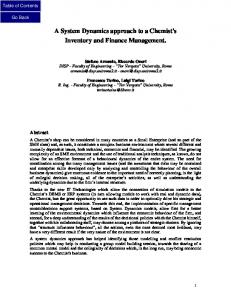
As a second example we show the post-modern jewelry by Rebekha Laskin for Formica Colorcore 1. Note the strong non-linearities in the form language. Not only have the objects been made suggestively through a process of cutting, they suggest to be cutting tools themselves.
Figure 2: Postmodern jewelry by Laskin.
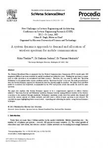
This can be contrasted against the Colosseum chair and stool by Charles Jencks, also post-modern (same reference). The form language is dominated by the circular forms arcs referring to the Colosseum. It is the form language of celestial movement and arcs that withstand the forces gravity. In the terminology we shall develop we call the Laskin jewelry an example of transferfunction nonlinearity. The Jencks furniture stems from transfer-function linearity.
1
See Postmodern Design by Michael Collins and Andreas Papadikis.
Figure 3: Colosseum chair and stool by Charles Jencks.
3. Plan of the work In this paper we shall argue along the following lines: •
to understand emotional aspects of meaning we must adopt a systems view, considering not only the artifact, but studying the joint behavior of the artifact and other systems components it interacts with; for example to understand the expression fear it is indispensable to consider the behavior of the predator or whatever causes the fear;
•
non-linear dynamics is a rich and growing field of knowledge which has been somewhat undervalued; one of the reasons we suspect is that linear systems seemed to offer certain advantages from an engineering point of view (easier to understand and to analyze); but progress in non-linear dynamics has offered new terminology and theories so both engineering and design can start exploiting non-linear dynamics;
•
our brains work in non-linear ways; moreover non-linear mechanisms can and will be embedded in the implementation of more and more intelligent dynamic systems; in other words: the non-linearity is all over the place anyhow;
•
non-linear means several things; we have to disentangle the notions involved, both theoretically and practically;
•
to move beyond the expression of anger, fear and attraction we need more concepts, notably (a) learning and (b) uncertainty.
In order to be as precise as possible, we start with disentangling the notions and meanings of the word "non-linear" first. We also illustrate what one can do with the notions thus coming to surface. Then we develop a classification scheme of behaviors, based on the linearity or nonlinearity of the components.
3. Disentangling concepts We divide the behaving objects with respect to their linearity to linear and nonlinear and with respect to the stream of information processing within to feed-forward and feedback. • Linear means having straight-line transfer functions, like f(x) = 3.x, as opposed to f(x) = x3, which is non-linear; let's call this "transfer-function linearity", or just transfer-linearity or linearity; • Feed-forward means doing cascaded information processing, like in a chain sensor → preamplifier → AD-converter → decision-module, as opposed to the chain gain-control → amplifier → gain-control which features a feedback cycle. This could refer to architecture linearity in a broad sense. Here we shall explore the advantages and disadvantages of each. Especially we have to look at the movement controllers and to the oscillators inside the agents (as we also call behaving products), because these can be viewed as the generators of movement. We look at controllers and oscillators both in living and in artificial systems. In this section we shall not do anything new, but the fact that we make the information accessible to the design community in our opinion has added value.
First we explain the concept of transfer-function linearity. We compare two different behaviors illustrated by two distinct aspects of a car, see the figure below.
Figure 4: Linearity (springs) and non-linearity (bumper).
We consider the suspension springs and the bumpers. The springs allow the car to move vertically in such a way that the harder it is pushed down (or the harder wheels are pushed up by the road bumps), the further the springs are compressed. A normal spring has this very simple behavior (it's called Hooke's law). Some more sophisticated springs are non-linear, the so-called progressive springs. The bumper behavior is definitively non-linear however. At low forces the bumper behaves elastic but at a certain force it certainly opposes the force, not moving. When the care bumps against an object, the forces will act shock-wise and the bumper is even supposed to break and absorb external energy. Unlike the spring, a crashed bumper will not release that energy anymore. The two transfer functions involved can be visualized as graphs. The ∆y denotes a vertical displacement, the ∆x a horizontal displacement. F means Force. Of course we are aware that the design of the real car is far more subtle than sketched here (dampers, active suspension etc.) but the point here is to illustrate linearity and non-linearity, not to engineer the most sophisticated suspensions.
Figure 5: Linear and non-linear transfer functions.
Next we discuss the concept of architecture linearity (feed-forward versus feedback). The first example illustrates the feed-forward case. Consider the power train of a car, such as the following abstract representation of a 1958 Chrysler Imperial (why we chose this car will become clear later). The flow of energy and its control is done in a straightforward left-to-right fashion. The gas throttle controls the engine. The engine delivers its power to a gear box. The gear box feeds into the Cardan shaft which serves to feed the engine's power in a flexible way to the rear axis. The rear axis is equipped with a clever device called the differential which serves to divide
the available power over the two wheels while preventing slipping. We call this architecture "feed-forward".
Figure 6: Feed-forward system (transmission).
For this car an innovative extra option was offered, in those days called the automatic pilot. Nowadays we call it cruise control. The NY Times announced in 1958 as follows: "Chrysler's auto-pilot provides a footless accelerator pedal" 2. The system's architecture is given in the figure below.
Figure 7: Feedback system (cruise control).
The user can adjust a speed dial and set it to a certain speed of his or her choice. The car then automatically tries to maintain this speed, independent of the wind and the road's gradient. It works as follows: a fly-ball governor measures the actual speed of the car. The (mechanical) level coming out of this device is compared to the speed dial setting. When there is a difference, this means that the throttle is adjusted automatically: when the speed dial value is more than the flyball value, the throttle is opened. If the fly-ball output exceeds the desired speed, the throttle closes somewhat to reduce the engine's power. The adjusted engine power will eventually result in a new speed value, and thus the loop is closed. We call this architecture "feedback". Abstracting away from the particular details of the cars with and without cruise control we arrive at the following block diagrams. 2
See //www.imperialclub.com/Yr/1958/specs.htm
Figure 8: Feedforward and feedback architectures.
Of course we are aware of a number of subtleties in the cruise control's design, such as the haptic feedback given to the pedal and the integration effect built-in. But the point here is to illustrate the difference between feed-forward and feedback. Ball [5] describes the historic relevance of this innovation as follows: The 1958 Chrysler Imperial brings control theory to the masses. First car to have cruise control: for the first time, the general public directly experienced closed loop feedback control in action - the slowdown error as the car climbs a hill, the gradual reduction of that error due to integral operation of the controller, the small but unavoidable overshoot at the top - and learned to trust and accept such systems. The Chrysler Imperial embodies the final supercession of Divine control, and today we are so comfortable with feedback control inducing stable dynamics that we barely notice how it permeates most aspects of our lives.
Note the mentioning of the term "stable dynamics": it hints to a delicate and complex issue to which feedback systems give rise: non-trivial dynamic behavior. The gradual reduction of the hill-climbing error and the overshoot are examples. But there is also the possibility of oscillation. Imagine a control system which is too eager in its reaction: the car goes slightly too fast, speed is immediately reduced, the car goes too slow, full throttle again, more overshoot etc. Usually this is undesired, but certain technical and biological systems precisely need such oscillatory behavior. The cruise control, a brake servo, are traditional linear feedback systems. There is a good reason why the engineers used to like transfer-linear systems and for how they used all their knowledge about feedback: they used it to exorcise the transfer-function non-linearities and hence get smooth, predictable, and non-oscillating behavior. This is what we called classical control.
4. Taxonomy of behaviors Consider an artifact A (product or robot or vehicle or agent) meeting an active entity B (user or predator or resource or system component) in its environment. We use the neutral term "agent" for both. Both agents A and B have sensors, processing elements, and actuators. In other words, each agent looks as follows: sensors → processing elements → actuators.
Some of the sensors may measure positions, such as the agents own position in space or its position relative to the other agent. Some of the actuators make the agents move, for example it may have legs, or a crawling body, engine-driven wheels, propulsion jets, etc. We study the behavior of a single agent first. Later we may study the combined behavior of two or more such systems. We assume it to move in some space S, for example a flat twodimensional surface, or perhaps a higher dimensional space of position parameters, velocity parameters, posture angles, color parameters, etc. When an agent moves, its position and its measurements will change in a dynamic way. To identify categories, we may systematically vary the properties of the agent(s), both the transfer-function linearity, which may or may not apply, and their architecture, which may be feed-forward only or which may include feedback. transfer function
architecture
expected behavior
linear
feed-forward
straight lines or conic sections
linear
feedback
stable control or oscillations
non-linear
feed-forward
jumping and bumping
non-linear
feedback
all of the above + learning, doubt and decision making
We made a number of trajectories to illustrate typical behaviors that arise from mechanisms based on the above four classes. We call them A, B, C, and D. Class A trajectories includes of course straight lines, but we also assume the straightforward behaviors of mechanisms such as linear resonance systems and the trajectories of circular motion such as gear wheels or and planets. Combining such movements in two directions gives Lissajous figures. We also include parabolas an ellipses, although not the graph of linear functions, they are the outcome of the linear differential equations that describe gravity.
Figure 9: Trajectories produced by systems with linear transfer functions and feed-forward only.
Although they are shown as sketches, they are derived from precise Mathematica [6] formulas, see footnote.3 Class B is about trajectories typically arising from classical control systems. For a system with certain eigen-frequency, the behavior may have a tendency to oscillate, but the oscillation fades out. That is what a stable control loop does. Alternatively, the system may oscillate and the oscillation grows without bounds. In control theory, that is considered poor oscillator design (also think of the Tacoma bridge disaster). We give the formulas of class B 4.
Figure 10: Trajectories produced by systems with linear transfer functions and feedback.
Class C is about systems with non-linear transfer function but with feed-forward only (no feedback loop). Adopting the non-linearity of a bumper, the trajectories include multiple bouncing, truncated oscillations, bouncing-ball parabola and the chaotic behavior of a ball on a circular billiard. We also give the formulas of C5
Figure 11: Trajectories produced by systems with non-linear transfer functions and feed-forward.
Finally, Class D trajectories are produced by systems with non-linear transfer functions with feedback. Essentially anything can happen (including A,B and C). Shown below is an oscillation which grows but stabilizes gradually, and another oscillation of the latter type processed by a non-linear transfer function. Certain systems can even show sudden changes of the mode of oscillation.
3
Top row: ParametricPlot[ {Sin[u],Cos[u]}, {u,0,6 Pi}], Plot[.5 t,{t,0,10π}], Middle: Plot[Sin[t],{t,0,10π}], ParametricPlot[{Sin[2u],Sin[3u]}, {u,0,2π}], Bottom: ParametricPlot[ {u,-u2},{u,-1,1}], ParametricPlot[ {.3u+.7Sin[u], Cos[u]},{u,0,6π}] 4 Plot[e-t/10 Sin[t],{t,0,10π}], Plot[.1e-t/10(t/10 Sin[t],{t,0,10π}] 5 ParametricPlot[{u,If[Mod[u,6]≥3, 2Mod[u,6],2(6-Mod[u,6])]},{u,0,6π}], Plot[If[Sin[t]≥.5,1,-1],{t,0,10π}], Bottom: ParametricPlot[{u,-2(Mod[ u,1]-.5)2},{u,0,4}] (billiard not as formula)
Figure 12: Trajectories produced by systems with non-linear transfer functions and feedback.
The formulas of the top row trajectories are included (the bottom one is just a sketch). The two given formulas describe specific solutions of the famous Van der Pol equation, found by the Eindhoven scientist Bathasar van der Pol in the 1920s6
5. Exploiting the power of non-linear systems As it has become clear so far, the complexity of a behavior that can be produced with the different systems gradually increases with adding transfer nonlinearity or feedbacks. Along with the taxonomy we have suggested a heuristic that the behavior produced with different types of systems can be associated with particular emotional or behavioral state. In this section we will suggest the type of behavior that can be produced by different well established nonlinear dynamics paradigms i.e. systems that include both, nonlinearity and feedback and show initial attempts to apply scientific approach to relating behavioral trajectory and emotional content. By intuition we may suggested that linear systems can produce smoothly changing patterns which we associate with peaceful and constant mood. Damped or excelling oscillations that are characteristic for the feedback systems with linear transfer elements are associated either with increase of amplitude and can be mapped to emotions like excitement, or anger or with relief in the emotional state for the damping oscillations. Feed forward systems with transfer nonlinearity, for instance multilayer perceptron networks, are universal approximators, as shown in [7], i.e. behavior with any functional dependency can be produced with such a system. We have shown examples of behavioral trajectories that result in repetitive, edgy, or bumping movements. So our intuition is that the produced behavior represents aggression or fear. These intuitions are to find more ground since recent psychophysical studies on the perception of emotional gaits reveal that the emotion-specific components derived from the kinematics analysis of motion data match features that have been described as fundamental for the visual recognition of emotions from gait [8]. Nonlinear feedback (dynamic) systems are capable of producing all of the varieties of behaviors, mentioned so far. In [9] it is argued, that the two most elementary behaviors of a nonlinear dynamic system are point attractive and limit cycle behaviors, corresponding to discrete and rhythmic movements. Dynamic systems have been used for movement pattern generators in neurobiology [10] pattern generators for locomotion [11], potential field approaches for planning of movements and as approaches for limb movement [12].
6
polmin=NDSolve[{u’’[t]-1(1-u[t]2)u’[t]+u[t] == 0, u[0] == 0.1, u’[0] == 0}, u, {t,0,80}] Plot[(Evaluate[u[t]/.polmin]),{t,0,40}], polmin=NDSolve[{u’’[t]-1(1-u[t]2)u’[t]+u[t] == 0, u[0]==0.1, u’[0] == 0}, u, {t,0,80}] Plot[(Evaluate[u[t]/.polmin])5,{t,0,40}]
In addition to the behaviors that the previously listed systems in our taxonomy are capable of, a system with such a complexity can not only show a smooth, edgy or repeating behavior, but also can naturally give rise to a completely novel behavior, and an emotional state. An example of complex behavioral trajectory that changes from an oscillatory to exponentially calming state in time is shown below:
Figure 13: Switching between behavioral states.
A point attractive dynamical system is designed such that the behavioral tasks are stable fixed points or attractors. The basic idea is to map the behavioral state of the system onto the mathematical state of a dynamics described by an appropriate differential equation. In the case of a point attractive dynamical system, the behavior is a discrete movement. A trajectory can be generated by integrating the dynamical system in time, as for instance proposed by the dynamic neural fields approach [3]. In this approach behavioral trajectory is formed by setting the dynamic parameters of the neural field such that the peak of activation on the field moves within the field in the direction towards the behavioral target. For rhythmic movements, the attractor is not a single point but a trajectory, as shown in the following figure, which actually represents the Van der Pol equations (see Section 4, Fig. D) in the state space:
Figure 14: Attractor for a rhythmic behavior.
Nonlinear coupled oscillator models as another example of nonlinear dynamical system show this type of dynamic attractors, i.e. a range of rhythmic behaviors can be produced with this models. A nonlinear dynamic system can have a combination of more than one point attractor
(associated with discrete movement) and more than one limit cycle (responsible for rhythmic behavior). Let us go back to the example from Section 2 referring to changing from a walk to a trot or gallop in a horse movement. The reason for that could be an external influence, or a spontaneous behavior of a horse. The switching among dynamical modes in a nonlinear motor control will happen suddenly but smoothly, without visible collision or stress reaction. The change can be explained with a highly nonlinear dynamic system, (a realistic model for the mammal brain) inside which a bifurcation occurrence, observed in the outside by a qualitatively novel behavior. Their combination can explain complex behavioral patterns as accurate reproduction of almost arbitrary human movements [13] but also more abstract behavioral processes or predicates as short term memory, and decision making. Besides the purely computational considerations, multiple brain research studies imply the relation of the emotion to movement and behavior. The amygdala has been consistently implicated in emotional functions (see [15,16,16]. Among all the weapons of contemporary science, only nonlinear dynamics methods and statistical methods have shown the potential for realistic modeling of brain functions and the resulting behaviors. One may conclude that indeed the nonlinear dynamics methods would be good for creating complex and emotional behaviors, but this is probably beyond the skills and the knowledge of a (present-day) designer. On the contrary, Omlor and Giese [8] show that the following nonlinear generative model will approximate emotional movement trajectory:
Where the xi is the i-th trajectory and sj is the j-th source signal., t is time and τ signifies delay (feedback parameter). Using these nonlinear equations and the followed analysis, Omlor and Giese [8] conclude that anger in walking is characterized by increases of the amplitudes of many joints, while sad walking is characterized by decreased arm movements. These results match closely with dynamic features that have been described in psychophysical studies on the perception of emotional gaits, which have extracted salient features from perceptual ratings.
6. Conclusions Although the examples of Sections 2 and 3 may appear somewhat naive and technologicallyinspired, the results and insights of Section 5 strongly indicate another and deeper connection: our movements are generated and processed by non-linear dynamic systems (in the brain). Next to the motivations of Section 2, additional motivation was triggered by early psychological studies [19,19]which has been illustrated with the animation available at 7 . Moreover, multiple brain research studies imply the relation of the emotion to movement and behavior.
7. References 1. Braitenberg, V. (1994) Vehicles: experiments in synthetic psychology, MIT Press, Cam-. bridge & London 2. Emilia I. Barakova and Tino Lourens “Efficient episode encoding for spatial navigation. International Journal of System Science”, vol. 36 No. 14 November 2005, pp. 887–895. 3.
Erlhagen, W. and Schoener G. 2001. Dynamic field theory of movement preparation. Psychological Review. 109, 3, 545-572
4. Mein Vorkurs am Bauhaus : Gestaltungs- und Formenlehre / von Johannes Itten 7
http://www.cs.brown.edu/people/black/Movies/heider.mov
5. Rowena Ball. Then and now: a world tour of non-linear dynamics, stability and chaos. University of Southern Queensland seminar, 31 July 2007. http://complexsystems.net.au 6. Stephen Wolfram. The Mathematica book, Fourth edition. 7. Hornik, K., Stinchcombe, M., and White, H. 1989. Multilayer feedforward networks are universal approximators. Neural Netw. 2, 5 (Jul. 1989), 359-366. DOI= http://dx.doi.org/10.1016/0893-6080(89)90020-8 8. Omlor L, Giese M A (2006) Extraction of spatio-temporal primitives of emotional body expressions. Neurocomputing, in press. 9. Schaal, S.;Kotosaka, S.;Sternad, D. (2000). Nonlinear dynamical systems as movement primitives, Humanoids2000, First IEEE-RAS International Conference on Humanoid Robots 10. A. I. Selverston, “Are central pattern generators understandable?,” The Behavioral and Brain Sciences, vol. 3, pp. 555-571, 1980. 11. G. Taga, Y. Yamaguchi, and H. Shimizu, “Self-organized control of bipedal locomotion by neural oscillators in unpredictable environment,” Biological Cybernetics, vol. 65, pp. 147-159, 1991 12. F.A. Mussa-Ivaldi and E. Bizzi, “Learning Newtonian mechanics,” in Self-organization, Computational
Maps, and Motor Control, P. Morasso and V. Sanguineti, Eds. Amsterdam: Elsevier, 1997, pp. 491-501. 13. Ijspeert, A.;Nakanishi, J.;Schaal, S. (2001). Trajectory formation for imitation with nonlinear dynamical systems, IEEE International Conference on Intelligent Robots and Systems (IROS 2001), pp.752-757. 14. Damasio, A. (1999). The Feeling of What Happens: Body and Emotion in the Making of Consciousness: Harcourt Brace. 15. LeDoux, J. E., & Phelps, E. A. (2000). Emotional networks in the brain. In M. Lewis & J. Haviland (Eds.), Handbook of Emotions (pp. in press). New York: Guilford Press. 16. Rolls, E. T. (1998). The Brain and Emotion: Oxford University Press. 17. Omlor L, Giese M A (2006) Extraction of spatio-temporal primitives of emotional body expressions. Neurocomputing, in press. 18. Heider, F., & Simmel, M., An Experimental Study of Apparent Behavior, American Journal of Psychology, 57:2, , (1944). 19. Michotte, A. (1950). The emotional significance of movement. In M. L. Reymert (Ed.),Feelings and emotions. New York: McGraw-Hill