Proceedings of the 44th IEEE Conference on Decision and Control, and the European Control Conference 2005 Seville, Spain, December 12-15, 2005
ThC04.2
Sensor Validation And Outlier Detection Using Fuzzy Limits Jari Näsi, Aki Sorsa and Kauko Leiviskä,
Abstract— In a continuous industrial process, the accuracy and reliability of process and analytical measurements create the basis for control system performance and ultimately for product uniformity. Validation of measured values is the key and a prerequisite to guarantee reliable measurements for process control. This application introduces the use of standard deviation and density function-based absolute limits. Limits are used to cut off outliers and weigh the reliability of the on-line measurement against more reliable, but seldom made, laboratory analysis. Absolute limits are accomplished with constant or adaptively updating fuzzy limits. The adaptive fuzzy limits are recursively updated in real time when a new measured value and reference analysis become available.
T
I. INTRODUCTION
HIS paper studies the validation and outlier detection of on-line measurements. Validation means the verification of the measurement with other information or measurements. An outlier is a measured value, which lies abnormally far from other values. The practical challenge is to validate a continuous measurement using its previous values and the reference signal. Several factors make it difficult to validate sensor data. The difference between slight sensor failures and noisy sensor readings is not easy to verify if the process dynamics are unknown. In the case of one on-line sensor, the Kalman filtering technique is the most usual approach. This technique extends to several other applications such as improving the accuracy of process variables data smoothing and parameter estimation. Kalman filtering assumes linear dynamic systems and uses weighted least squares as an objective function. Methods also exist for sensor malfunction detection. Rollins et al. [10] developed a method to handle biased measurements in general fashion exploiting the gross error detection approach. The authors have developed an algorithm for merging online measurements and an infrequent reference signal into one signal. This algorithm is presented in detail in [6] and has three parts: pre-processing, confidence level estimation and the calculation of the estimate (Fig. 1). This paper focuses on the pre-processing of data and particularly on the limits used in outlier detection. The methods presented in Manuscript received February 25, 2005. This work was supported in part by National Technology Agency (Tekes) and the Outokumpu Foundation in Finland. All authors are with University of Oulu, Control Engineering Laboratory, FIN-90014 Oulun yliopisto, Oulu, Finland (Corresponding author Jari Näsi; e-mail:
[email protected]).
0-7803-9568-9/05/$20.00 ©2005 IEEE
7828
this paper extend the usability and functionality of preprocessing by giving time-varying, process conditiondependent limits. Naturally, more realistic pre-processing also enhances the on-line use of the whole system. The outlier detection is performed by a classifier, which uses absolute and fuzzy limits. Absolute limits define the minimum and maximum allowable values of the measured variable. The absolute limits can be determined by using the normal distribution or density function. These methods are further discussed in chapter 3, where artificial data is used to illustrate the differences between the methods. As the absolute limits can only be used to produce information on whether the measurement is acceptable or unacceptable, the fuzzy limits are used to soften the change between these two states. Furthermore, time-varying fuzzy limits can be used to handle changing process conditions and measurement uncertainty. Chapter 4 discusses different methods for determining fuzzy limits. Instead of artificial data, real process data is used to highlight the differences between the different methods. The data used consists of redundant sensor data from the electrolytic zinc production process. An evaluated analyzer measures the Fe2+ content in a dissolution reactor. This measurement occurs every ten minutes by titration. Deterioration of the measurement device causes drifting and occasional breakdowns. The value measured is used for process monitoring, not for control and if working properly, it gives useful information about the process conditions. Chapter 5 compares the methods developed and describes how the measurement replacement operates after the determination of the absolute and fuzzy limits. Continuous measurement
Xm Absolute and fuzzy limits
Signal pre -processing Bias correction
Classifier
Xc
Confidence level Confidence level Laboratory analysis
Cm
Cl
Confidence level based reasoning
Xe
Optimal estimate
Xl
Fig. 1. Signal processing for the optimal estimate.
II. METHODS A. Uncertainty in the Measurements The term measurement uncertainty means the doubt about
the validity of the measurement and it is also a measured parameter. Uncertainty is normally associated with the measured value. Another definition is the probability of a reading lying inside a given range on either side of the mean value. Uncertainty can also be understood as a distribution [11]. Normal distribution is a common way to represent the distribution of measured values and the uncertainty involved. Confidence limits typically represent the magnitude of a random error in a measurement. Usually, in the case of the normal distribution, 95 % confidence limits are used. [9] Estimation of uncertainty uses variables linked to the measurement such as process noise, sensor drift, sensor malfunction. The SEVA approach combines these factors into a value that describes the uncertainty of a measurement [3]. Sensor malfunction detection can also augment the estimation of uncertainty in the SEVA approach. This system classifies sensor failures and estimates their impacts on signals and uncertainties [2]. However, these variables are not necessarily easy to define. Various control methods can be effective in dealing with uncertain measurements, but measurement noise and errors affect their performance. Outliers constitute a challenging problem and detecting them is much easier for human than for a computer. The following chapter deals with outlier detection. In this study, uncertainty is associated with process dynamics, instead of estimating it from certain variables. Process dynamics originate from the data as statistical values or from expert knowledge. This paper uses the term “confidence” instead of “uncertainty”. B. Outlier Detection Most outlier detection methods start from the assumption of identically and independently distributed (i.i.d) data, where the mean and variance describe the statistics of the data [5]. A commonly used method for outlier detection is to look for observations that deviate more than three times the standard deviation from the mean. This is the usual “3δ edit rule”. If outliers are present, this method includes a basic difficulty: outliers lead to biased estimates for both the mean and the standard deviation. Even a single outlier is enough to bias the mean, and the situation is made worse with multiple outliers, especially if they are located on the same side of the mean. For example, [4] the exponentially weighted moving average (EWMA) used for detecting possible outliers from on-line consistency measurements. Unfortunately, this method is also sensitive to outliers and after stable process conditions even normal process changes are detected as outliers. On the other hand, after real outliers, the limits become so wide that following outliers are accepted as true values. To overcome these problems, one possibility is to replace the mean with the median and the standard deviation with the median absolute deviation from the median. This is the Hampel identifier and it is one of the most efficient methods.
7829
Reference [1] proposes two further modifications to increase the sensitivity in detecting outliers: modified scaling and consistent modified scaling. According to [5] there are also a group of methods based on the assumed process models utilizing maximum likelihood methods and the Kalman filter. They also present an on-line filter-cleaner that combines the properties of outlier detection methods and online filters. In addition, wavelet transform has been used in on-line filtering and outlier detection [7]. Outlier detection can also benefit from statistical process control (SPC), such as the calculation of the cumulative sum or using control charts. Statistical process control assumes that: 1) the mean of the process measurements is constant; 2) the deviation of the measurements is constant; 3) measurements are independent. In the process industry, these prerequisites may be problematic, because the mean and deviation vary as a function of time or as a consequence of disturbances and breakdowns. Correlation between measurements shows as a trend in the control charts, which complicates the interpretation to control the process. In continuous processes, almost all the variables have some temporal correlation, even if a process is under statistical control [8]. This paper introduces an adaptive fuzzy approach using a modified standard deviation and 95% confidence limits. In on-line applications, this makes the updating of outlier limits possible, when process conditions change. III. ABSOLUTE LIMITS WITH NORMAL DISTRIBUTION AND DENSITY FUNCTION Absolute limits define the scale, where the process parameter can vary under normal process conditions. The upper limit gives the maximum value, which is reliable. If a measurement device gives larger values than this, they should be ignored and replaced with other process information. In the same way, smaller values than minimum should be replaced. Experts can define the limits manually, but they can be also defined automatically from process data. This chapter compares the use of normal distribution and density function for this purpose. To illustrate the determination of the limits for outlier detection, a data set of measurements and reference values was generated (Fig. 2). The measurements follow the sinfunction with added noise and random spikes. A. Normal distribution The mean value and standard deviation of the data define the normal distribution. The mean value is
15
0.18 Alaraja Minimum
0.16
Yläraja Maximum
0.14
10
0.12 0.1 0.08 0.06
5
0.04 0.02
0
0
50
100
150
200
250
300
350
400
450
0
500
Fig. 2. Generated data set (measurements and reference values) with random spikes.
m=
1 n , ∑ xi n i =1
(1)
where m is the mean value, n is the number of measurements and xi is the i:th measurement. The standard deviation is
σ=
1 n ∑ ( xi − m)2 . n i=1
0
5
10
15
20
25
Fig. 3. Absolute 2σ limits from the normal distribution for the data shown in Fig. 2.
By using a density function, the limits obtained represent the actual process better. Moreover, the use of the density function is flexible and gives the chance to use a priori knowledge. In this case (Fig. 2), it is more likely that the measurement has a spike downwards (zero value) than a spike upwards. It can be emphasized by cutting out, for example, only one percent of the higher values and four percent of the lower values, retaining the original property of 95 percent of measured values lying between the limits.
(2)
Normalized density function
Cumulative sum
0.3 1
The normal distribution is now 1 ( x − m )2 . N (x) = exp( − ) 2σ 2 σ 2π
0.25 0.8
(3)
0.2 0.6 0.15
When using a normal distribution, about 95 percent of the measured values lie inside m ± 2σ (Fig. 3). If the data used is not pre-processed, the use of 2σ-limits is justified, otherwise, for example, the use of 3σ-limits as absolute limits can be considered. B. Density function The density function requires classified data. Fig. 4 shows the normalized number of measurements in each class both as a histogram and as a cumulative sum. Two vertical lines in the cumulative sum diagram show the locations for 95% confidence limits. The upper limit corresponds to a location where the cumulative sum exceeds the value of 0.975. The lower limit corresponds to a value of 0.025. Comparing the density function and normal distribution (Fig. 3 and Fig. 4), the upper limit is almost the same regardless of the method. However, the lower limit calculated from the normal distribution is lower than the one from the density function. This is due to the assumption that the data is distributed equally around the mean value when using the normal distribution. This is not always the case as shown on the left-hand side of Fig. 4.
7830
0.4 0.1
0.2
0.05
0
0
5
10
15
20
25
0
0
5
10
15
20
25
Fig. 4. Absolute 95% confidence limits from the density function.
IV.
FUZZY LIMITS
Fuzzy limits narrow the area limited by absolute limits. The efficient use of fuzzy limits, combined with the absolute limits and reference measurement creates the basics to make the reliable calculation of the “optimal” signal. This chapter compares the use of constant and adaptive fuzzy limits. The adaptation of fuzzy limits occurs with two different methods based on a standard deviation. A. Constant fuzzy limits Equation 4 defines constant fuzzy limits as a fraction of the range of the variable. Experts can see the width of the fuzzy limits. In the case of the processes studied, a 10 % fraction of the variables range was found to be appropriate.
X min, fuz = X min + β ( X max − X min ) X max, fuz = X max − β ( X max − X min )
Measurement
(4)
Above, β is a coefficient describing the width of the fuzzy zone. If the fuzzy limits are constant, the detection of an invalid measured value depends on the process conditions. If the measured values drift closer to the limits, the deviating ones are more likely to lie in the fuzzy region. In Fig. 5, there is a trend of measurements drifting closer to the upper limit. Seven values inside the circles are possible outliers; three of them occur when the measured values are far from the limits and four when they have drifted closer to the upper limit. Even though the deviations are of about the same magnitude, the four latter values are classified as possible invalids. Keeping this in mind, the fuzzy limits should be flexible and change with the process conditions. B. Adaptive fuzzy limits from the standard deviation Adaptation means here that the fuzzy limits change when the process conditions (mean and deviation of measurements) change. To use the standard deviation in adaptation, a time window of reasonable length has to be defined. The standard deviation inside the window can be obtained from equations 1 and 2. The fuzzy limits are now xref ± 2σ w, where σw refers to the standard deviation inside the time window. Instead of connecting fuzzy limits to the absolute limits, adaptive limits are connected to the reference analysis. This approach suffers from the fact that fast variations in the standard deviation significantly affect the limits. The limits expand and possibly invalid measured values appear valid. For example, in the data set, where an on-line measurement device deteriorates and gives an unstable signal, fuzzy limits expand outside the absolute limits (Fig. 6). One way to improve this approach is to eliminate deviating measured values before the determination of the fuzzy limits. This, however, requires more reasoning and makes the overall system more complex.
Limits and reference measurement Fuzzy limit Absolute limit Reference Absolute limit Fuzzy limit
Fig. 6. Fuzzy limits determined from the standard deviation (absolute limits base on a longer time period from the same measurement device). Calculation works properly with normal data, but when problems appear, limits expand.
C. Adaptive fuzzy limits from the modified standard deviation Equations 5 and 6 show a modified standard deviation that decreases the effect of outliers on the calculated fuzzy limits. The weight of each measured value depends on its deviation from the mean.
σm =
1 N ∑ α ( xi − m)2 N i =i
(5)
where σm is the modified standard deviation, N is the number of measurements in a window and α is a weighing coefficient.
α = e− a ( x − m)
2
, where a is a parameter. i
Upper absolute limit
,
(6)
Possible invalids
Equation 6 needs a value for the parameter a. A good fitting for the coefficient is obtained, if xi - m = σd results in a = 0.5 (Fig. 7). The deviation, σd, depends on the absolute limits
Upper fuz zy limit
valids
σd =
Fig. 5. Constant fuzzy limits with drifting process conditions.
7831
X max − X min , 4
(7)
Abs. limit
1
0.8
0.6
α 0.4
Abs. limit
σd
0.2
0 -4
-3
-2
-1
0
Reference Measurement
1
2
3
4
Fig. 9. Data used in method comparison.
xi - m
V. RESULTS
Fig. 7. The determination of coefficient a.
Combining Equations 6 and 7 leads to
a=−
ln 0,5 ,
(8)
σ d2
Using the modified standard deviation leads to better results (Fig. 8). The adaptive fuzzy limits are always inside the absolute limits, because the outliers do not affect the modified standard deviation so much. The significance of one deviating value decreases and the changing fuzzy limits apply directly to the measured values without any prior reasoning. Measurement
Limits and reference measurement Absolute limit Fuzzy limit
Fuzzy limit
In this chapter, methods for determining fuzzy limits are compared. The data used consists of 12000 measurements. This data is used to initialize the necessary parameters while the method comparison is carried out by a data set consisting of 2000 measurements (Fig. 9). Part of this data set has already been used in chapter 4 to highlight the differences between the different methods. The initialization is carried out by calculating the absolute limits and the initial values for the fuzzy limits. The absolute limits are calculated by using the density function (Fig. 9). The total fraction of invalid measurements is 5%. However, the data set represents the case of a malfunctioning sensor where the deviation between the reference signal and measurements becomes very large and the fraction of invalids is expected to increase. The performance evaluation of different methods is carried out here by summing up the number of measurements in different regions (valid, fuzzy and invalid). From real process data it is hard to calculate the actual number of measurements in different regions. However, according to our estimation, 25 percent of measurements belong to either in fuzzy or invalid regions. The numbers of measurements in different regions with different methods are tabulated in Table 1. The challenges with constant fuzzy limits, discussed in chapter 4, can be observed in the results. A modified deviation gives results closest to the estimated results. Using a standard deviation seems to detect too few possible outliers, which can be explained by comparing Figs. 6.and 7. The fuzzy limits expand far enough to match up to the absolute limits and therefore possible outliers are not detected. Table 1. The numbers of measurements in different regions with different methods. N:O MEASUREMENTS USED FUZZY LIMIT Valid Fuzzy Invalid
Absolute limit
Fig. 8. Adaptive fuzzy limits determined from the modified standard deviation. Note that the scale in the lower figure differs from Fig. 6.
Constant 1742 (87%) Standard deviation 1627 (81%) Modified deviation 1449 (72%)
56 (3%) 171 (9%) 349 (18%)
203 (10%) 203 (10%) 203 (10%)
A. Measurement replacement After the determination of the absolute and fuzzy limits, a
7832
classifier (Fig. 1) detects the outliers and deviating values and replaces them with an estimate. If the measurement is inside the fuzzy zones, the output from the classifier is a weighted average of the actual measured value and the reference value.
X C = wm X m − wref X ref
(9)
where wm and wref are the weights of the measurement and the reference, Xm is the measured value and Xref is the reference value. If the measured value is inside the fuzzy limits, the classifier considers it valid. In that case, the weight of the measurement is 1. If the measured value is beyond the absolute limits, the weight of the measurement is 0. Between the valid and invalid zones lies a fuzzy zone, where the weight of the measurement decreases from 1 to 0 (see also Fig. 5). As a result, the weight of the actual measured value is ⎧ ⎪0, X < X min ⎪ ⎪ f1 , X min < X < X min, fuz (10) ⎪ wm = ⎨1, X min, fuz < X < X max . fuz ⎪ ⎪f , X max, fuz < X < X max ⎪ 2 ⎪0, X > X max ⎩
device is not correct and includes a bias (otherwise measurement shows process variations correctly), the reliability of the measurement may decrease in an unexpected way. A clear benefit of adaptive fuzzy limits is the adaptation to varying process conditions. Unfortunately, if the limits are calculated directly from the moving standard deviation, highly deviating values expand the fuzzy limits and make them useless. In the case of modified deviation, the benefit of the calculation is a controlled response to the changing signal: • In the case of small changes (process is stable and measurement device works well) the weight used gives large reliability values for the signal and allows wide confidence limits. • If the process varies after stable conditions, the measured changes are accepted as true. In addition, process disturbances cause a reasonable response in the adaptive limits. • A greater variation in signal (possible outlier) is compensated by the gradual diminution of the weighting factor. • Peaks, caused by outliers and strong process disturbances, will be given small weighting and instead of widening, adaptive limits will narrow and allow only those values close to the reference be accepted as true. REFERENCES [1]
where f1 and f2 are the membership functions describing the behaviour of the weight inside the fuzzy zone. The weight of the reference value is simply:
wref = 1 − wm .
(11)
The calculation of the bias correction, confidence levels and optimal estimate is discussed in detail in [6]. VI. DISCUSSION Two methods were compared for the calculation of the absolute limits. Density function-based limits are less sensitive to non-optimally divided values. This method also makes it possible to react if one side of the distribution is more heavily weighted. The functionality of the fuzzy limits was tested with real process data. Constant fuzzy limits work as a softener between reliable and non-reliable measurements, but their action is dependent on process conditions. If real process values are close to the absolute limit, deviating measurements are easily classified as non-reliable (they are inside the fuzzy zone). To prevent these problems, adaptive fuzzy limits are connected to the reference analysis. Drifting of the measurement (biasing after deterioration of measurement devise) away from the reference is also prohibited. On the other hand, if the calibration of the measurement
7833
Chiang, L.H., Pell R.J., and Seasholtz, M.B., Exploring process data with the use of robust outlier detection algorithms. Journal of Process Control 13(2004) pp. 437-449. [2] Fry, A.J. (2001) Measurement Validation via Expected Uncertainty. Measurement, vol. 30, pp.171-186. [3] Henry, M.P. & Clarke, D.W. (1993) The Self-validating Sensor: Rationale, Definitions and Examples. Control Engineering Practice, vol. 1, no. 4, pp.585-610. [4] Latva-Käyrä, K. (2003) Dynamic validation of on-line Consistency Measurements. Tampere University of Technology, Publications 442, 106 p. [5] Liu, H.C., Shah, S., and Jiang, W., On-line outlier detection and data cleaning. Computers and Chemical Engineering 28(2004) pp.16351647. [6] Näsi, J. & Sorsa, A., On-line measurement validation through confidence level based optimal estimation of a process variable. Report A No 25, Control Engineering Laboratory. [7] Nounou, M.N., and Bakshi, B.R., On-line multilevel filtering of random and gross errors without process models. American Institute of Chemical Engineering Journal 45(1999) pp.1041-1058. [8] Oakland, J.S. & Followell, R.F., 1990. The book, Statistical process control. A practical guide. Heineman Newnes, Oxford, 431 p. [9] Pyle, D (1999). Data Preparation for Data Mining. Morgan Kaufmann, San Francisco, California. [10] Rollins, D.K., Devanathan, S. & Bascuñana, V.B. (2002) Measurement Bias Detection in Linear Dynamic Systems. Computers and Chemical Engineering, vol. 26, pp.1201-1211. [11] Weiss, S.M. & Indurkhya, N. (1998) Predictive Data Mining - A practical guide. Morgan Kaufmann Publishers, Inc. San Francisco, California.