Separation of Concerns in Feature Modeling: Support and Applications

Separation of Concerns in Feature Modeling: Support and Applications Mathieu Acher University of Namur PReCISE Research Centre, Belgium [email protected]

Philippe Collet Philippe Lahire Université Nice Sophia Antipolis, France {collet,lahire}@i3s.unice.fr

Abstract

Computer Science Department Colorado State University, USA [email protected]

SPL and their valid combinations; it is basically an ANDOR graph with propositional constraints [12, 27, 32]. FMs are becoming increasingly large and complex. A contributing factor to their growing complexity is that FMs are being used not only to describe variability in software designs, but also variability in wider system contexts, at different times in the development and in different parts of the system structures [15, 19, 22, 24, 35]. As a result, the list of concerns that may be considered in an FM is very comprehensive [8, 34] ranging from hardware description [19], organizational structure [24], business or implementation details [22]. In practice, the concerns are related in a variety of ways and there can be hundreds of features whose legal combinations are governed by many and often complex rules. The automated extraction of FMs from large implemented software systems now produces very large FMs. As an extreme case, the variability model of Linux exhibits more than 6000 features [29]. It has been observed that maintaining a single large FM for the entire system may not be feasible [14, 23]. On the one hand, several FMs may be originally separated and combined: It is the case when one describes the variability of (sub-)systems that are by nature modular entities (e.g., software components or services [5]), when independent suppliers describe the variability of their different products in software supply chains [13, 16], or when a multiplicity of SPLs should be integrated [14, 15]. On the other hand, it can be the intention of an SPL practitioner to modularize the variability description of the system according to different criteria or concerns. It is the case when external variability is distinguished from internal variability [22, 23], when FMs are organized in layers [19], or when a simplified representation of an FM (a view) has been tailored for a specific stakeholder, role, task [17]. With FMs being increasingly complex, describing various concerns of an SPL and handled by several stakeholders (or even different organizations), managing them with a large number of features that are related in a variety of ways is intuitively a problem of Separation of Concerns (SoC) [9, 30]. First, composing support is needed to group and evolve a set of similar FMs, or

Feature models (FMs) are a popular formalism for describing the commonality and variability of software product lines (SPLs) in terms of features. SPL development increasingly involves manipulating many large FMs, and thus scalable modular techniques that support compositional development of complex SPLs are required. In this paper, we describe how a set of complementary operators (aggregate, merge, slice) provides practical support for separation of concerns in feature modeling. We show how the combination of these operators can assist in tedious and error prone tasks such as automated correction of FM anomalies, update and extraction of FM views, reconciliation of FMs and reasoning about properties of FMs. For each task, we report on practical applications in different domains. We also present a technique that can efficiently decompose FMs with thousands of features and report our experimental results. Categories and Subject Descriptors D.2.2 [Software Engineering]: Design Tools and Techniques General Terms Design, Languages, Theory

1.

Robert B. France

Introduction

The goal of software product line (SPL) engineering is to produce a family of related program variants for a domain [23]. SPL development starts with an analysis of the domain to identify commonalities and differences between the members of the product line. A common way is to describe variabilities of an SPL in terms of features which are domain abstractions relevant to stakeholders and are typically increments in program functionality [8]. A Feature Model (FM) is used to compactly define all features in an

[Copyright notice will appear here once ’preprint’ option is removed.]

1

2012/3/2

An FM defines a set of valid feature configurations. A valid configuration is obtained by selecting features so that i) if a feature is selected, its parent is also selected; ii) if a parent is selected, all the mandatory subfeatures, exactly one subfeature in each of its Xor-groups, and at least one of its Or groups are selected; iii) propositional constraints hold. For example, in Figure 1a, { A, B, C, F, P, S, T, W} is a valid configuration, the features D and F cannot be selected at the same time and E cannot be selected without C due to the parent-child relation between E and C.

to manage a set of inter-related FMs [2]. Second, some complementary decomposing support is as important to reason about local properties or to support multi-perspectives of a typically large FM [4]. Due to the complexity of FMs, SoC support should be soundly defined and automated as much as possible. In previous work, we designed a set of composition (insertion, merging, aggregation) [2] and decomposition (slice) [4] operators.Their semantic properties were precisely defined in terms of configuration set and feature hierarchy, and fully automated techniques were developed to synthesize FMs. Using these operators separately has practical but limited interests. In many scenarios and case studies, an SPL practitioner rather needs to combine both techniques and perform sequences of composition and decomposition, while reasoning about intermediate results. In this paper, we show how the combined use of composition and decomposition operators forms a consistent and powerful support for SoC in feature modeling. We describe several novel applications of the operators, detailing the obtained benefits. These applications comprise i) the corrective capabilities of the operators themselves, ii) view extractions and updates on FMs, with the benefit of handling cross-tree constraints, iii) reconciling FMs that come from different stakeholders or organizations, and iv) reasoning about two kinds of variability to check important properties (realizability, usefulness) of an SPL. For each application, we report on practical use in different case studies. We revisit and implement some existing works with our operators and we report better results either in terms of capability or scalability. Furthermore, we present a technique that can efficiently decompose FMs with thousands of features and outperforms our previous implementation based on binary decision diagrams.

2.

D EFINITION 1 (Configuration Semantics). A configuration of an FM g is defined as a set of selected features. JgK denotes the set of valid configurations of the FM g and is thus a set of sets of features. FMs have been semantically related to propositional logic [12]. The set of configurations represented by an FM can be described by a propositional formula φ defined over a set of Boolean variables, where each variable corresponds to a feature (see Figure 1c for the formula corresponding to the FM of Figure 1a). The translation of FMs into logic representations allows one, as we will see in the next sections, to use reasoning techniques for automated FM analysis [10].

3.

Composition and Decomposition Support

In previous work [2, 4], we designed a set of composition and decomposition operators that produce a new FM from one or more than one input FMs. We have defined the semantics of these operators in terms of: configuration semantics We consider that the primary meaning of an FM, known as its configuration semantics, is a set of legal configurations – sets of selected features that respect the dependencies entailed by the diagram and the cross-tree constraints. We thus define the semantics of each operator in terms of the relationship between the configuration sets of the input FMs and the resulting FM.

Background: Feature Models

FMs were first introduced in the FODA method [19], which also provided a graphical representation through Feature Diagrams. FMs are now widely adopted with support of formal semantics, reasoning techniques and tooling [8, 10, 12, 27]. An FM defines both a hierarchy, which structures features into levels of increasing detail, and some variability aspects expressed through several mechanisms. When decomposing a feature into subfeatures, the subfeatures may be optional or mandatory or may form Xor or Or-groups. In addition, any propositional constraints (e.g., implies or excludes) can be specified to express more complex dependencies between features. We consider that an FM is composed of a feature diagram coupled with a set of constraints expressed in propositional logic. Figure 1a shows an example of an FM. The feature diagram is depicted using a FODA-like graphical notation used throughout the paper. The hierarchy of an FM is represented by a rooted tree G = (F, E, r) where F is a finite set of features and E ⊆ F × F is a finite set of edges (edges represent topdown hierarchical decomposition of features, i.e., parentchild relations between them) ; r ∈ F being the root feature.

feature hierarchy Another important property of an FM is the way features are organized – reflected in the feature hierarchy. We recall that two FMs can have identical configuration semantics, yet different hierarchies and thus ontological meaning [10, 29, 32]. As a result, we consider that the feature hierarchy should also be part of the semantics of the operators. 3.1

Aggregate

The aggregate operator supports cross-tree constraints between features so that separated FMs can be inter-related. The input FMs are aggregated under a synthetic root syntheticf t so that the root features of input FMs are childmandatory features of syntheticf t . In addition, the propositional constraints are added in the resulting FM. For example, the aggregate operator can be used to compose four FMs together with constraints (see Figure 5, page 6). The properties of the aggregated FM heavily depends on the set of propositional constraints used during the aggre2

2012/3/2

fm1 W P Optional

Mandatory

T

U

Xor-Group Or-Group

R S constraints

V

E implies D R implies E D excludes F S implies (F and not E)

A B

(a) FM: FODA-like representation

C E

D F

φf m1 = W // root ∧W ⇔P ∧ W ⇔T Jf m1K = { ∧ U ⇒ W // optional {A, B, C, D, E, P, R, T, U, W }, ∧ V ⇒ T ∧ A ⇔ T // mandatory {A, B, C, F, P, S, T, U, W }, ∧A⇔B∧ A⇔C {A, B, C, D, E, P, R, T, W }, ∧D⇒A {A, B, C, F, P, S, T, V, W }, ∧E ⇒C∧ F ⇒C {A, B, C, F, P, S, T, U, V, W }, // Or-group ∧P ⇒R∨S {A, B, C, F, P, S, T, W }, R⇒P ∧ S⇒P {A, B, C, D, E, P, R, T, V, W }, ∧ // constraints {A, B, C, D, E, P, R, T, U, V, W } ∧ E ⇒ D ∧ R ⇒ E } ∧ D ⇒ ¬F ∧ S ⇒ (F ∧ ¬E) (b) corresponding set of configurations

(c) corresponding propositional formula

Figure 1. FM, set of configurations and propositional logic encoding merged hierarchy should be retained. The problem of choosing a hierarchy from amongst a set of hierarchies can be formulated as a minimum spanning tree problem (see details in [1]). An example of merge operation in intersection mode is given in Figure 8, page 7.

gate. It may lead to situations where the aggregated FM does not represent any valid configuration or includes dead or core features (see Definition 2). We consider that the aggregate operator is purely syntactical. As we will see, other complementary techniques can be applied in case an SPL practitioner may want to simplify the aggregated FM or to reason about its properties. 3.2

3.3

Slice Operator

The slice operator aims at simplifying or abstracting FMs by focusing on selected aspects of semantics. The overall idea behind FM slicing is similar to program slicing [36]. Program slicing techniques proceed in two steps: the subset of elements of interest (e.g., a set of variables of interest and a program location), called the slicing criterion, is first identified; then, a slice (e.g., a subset of the source code) is computed. In the context of FMs, we define the slicing criterion as a set of features considered to be pertinent by an SPL practitioner while the slice is a new FM.

Merge

The merge operator is dedicated to the composition of FMs that exhibit similar features (i.e., features with the same name). In this case, the merge operator can be used to merge the overlapping parts of the FMs and then to obtain an integrated FM. The merge uses name-based matching: two features match if and only if they have the same name. Configuration Semantics. The properties of a merged FM produced by an application of the merge operator are formalized in terms of the sets of configurations of input FMs. Several modes are defined for the merge operator. We only describe here the modes that we will use in the remainder of the paper. The intersection mode is the most restrictive option: the merged FM, F Mr , expresses the common valid configurations of F M1 and F M2 . The merge operator in the intersection mode is denoted as follows: F M1 ⊕∩ F M2 = Result. The relationship between a merged FM Result in intersection mode and two input FMs F M1 and F M2 can be expressed as follows:

W P

T

R

A

S

constraints B

C

D

constraints E implies D D implies E

E

F

(a) [[fm2]] = {{A, B, C, D, E},{A, B, C, F}}

E implies D R implies E

U

V

A B

C E

D F

(b) [[fmAll]] = [[fm1]]

Figure 2. Two slice operations on fm1 (see Figure 1a)

JF M1 K ∩ JF M2 K = JResultK

Configuration Semantics. We define slicing as a unary operation on FM, denoted ΠFslice (F M ) where Fslice = {f t1 , f t2 , ..., f tn } ⊆ F is a set of features. The result of the slicing operation is a new FM, F Mslice , such that: JF Mslice K = {x ∩ Fslice | x ∈ JF M K } (called the projected set of configurations).

Another merge operator, called diff, is denoted as F M1 ⊕\ F M2 = Result. The following defines the semantics of this operator: JF M1 K\JF M2 K = {x ∈ JF M1 K | x ∈ / JF M2 K} = JResultK Hierarchy. Several FMs, with different hierarchies, can represent the same set of configurations [10, 29, 32]. So in particular several merged FMs can be produced and consistently represent the expected set of configurations while having different hierarchies. Intuitively, the more a parent-child relation occurs in the input FMs, the more an edge in the

Hierarchy. Intuitively, the hierarchy of F Mslice is such that features are connected to their closest ancestor if their parent is not part of the slicing criterion. A formal definition can be found in [1]. Two examples of slice operation are given in Figure 2. 3

2012/3/2

Case study À Composing Multiple Variability Artifacts (domain: medical imaging, grid computing ; stakeholders: medical imaging/grid experts) [5] Á Modeling Variability From Requirements to Runtime (domain: video surveillance (VS) systems ; stakeholders: VS expert, software engineer) [6] Â Management of Product Line and Software Variability (domain: any ; stakeholders: products manager, software engineer) [22]

Concerns the variability is described at different places of the workflow, describing various concerns of connected services

Complexity dozens of FMs (up to 30), hundreds of inter-related features (up to 400)

the modeling of requirements and software variability is explicitly separated in two FMs, VSAR and PC

à Reverse Engineering FMs (domain: component and plugin based systems, stakeholder: software architect) [3]

multiple variability sources (including architect knowledge) are combined to construct semi-automatically an FM

2 FMs, 77 features and 108 configurations in VSAR, 51 features and 106 configurations in PC, 39 constraints. 2 FMs, 25 features in f mP L , 11 features in f msof tware , 13 constraints ; 92 features and 158 constraints ; the number of valid configurations varies from ≈ 1011 to ≈ 106 ;

two kinds of variability (software and product line) are specified and maintained in two separated FMs f mP L and f msof tware

Figure 3. SoC in the case studies Technique Updating FM Views

Supporting Multiple Perspectives Reconciling FMs Reasoning about Two Kinds of Variability

Description several FM views are inter-related: The variability information is kept up-to-date in the different views, possibly by correcting some anomalies introduced by some constraints given an FM or a set of FMs, a stakeholder wants to focus only on a specific concern related to its expertises, role, task two (or more than two) FMs cannot be directly compared or merged: They are reconciled by removing unnecessary details two FMs describing two variability concerns are inter-related: Reasoning techniques are applied to reason about their relationships

Operators aggregate, slice

Application ÀÁÂÃ

aggregate, slice slice, merge

À

aggregate, slice, merge,

ÁÂ

ÀÃ

Figure 4. SoC in feature modeling

4.

Applying Separation of Concerns

terizes each technique, reports the operators involved in the realization of the technique as well as the practical use in case studies. The numbers correspond to the different case studies described in Figure 3, including the application domain, the stakeholders involved, the concerns considered as well as the complexity of FMs.

Given these composition and decomposition mechanisms, we now argue that these operators, together with other reasoning and editing operators, form a consistent and powerful support for SoC in feature modeling. Several usage scenarios can be envisaged: • When an FM is decomposed into smaller FMs (using the

4.1

slice operator), one may need to reason about the different sets of configurations or simply modify the smaller FMs. The composition operators can be applied afterwards to recompose the smaller FMs ;

Corrective Capabilities

Manual or automatic creation of FMs may generate anomalies in them. Generally, these anomalies are regarded as a negative property of an FM since it can easily decrease its maintainability or understandability.

• When some FMs are composed with constraints (using

D EFINITION 2 (Dead and Core features). A feature f of an FM is dead if it cannot be part of any of the valid configurations. A feature f of an FM is a core feature if it is part of all valid configurations.

the aggregate operator), one may need to simplify, redecompose or check the satisfiability of the resulting composed FM ; • Before merging two FMs, one may need to reconcile

(or align) the two FMs in case the hierarchy and the vocabulary used in the two FMs differs ; Beyond these simple examples, we now show that though the sole use of the composition / decomposition operators has practical interests, the area of applications grows when these operators are combined together1 . The following sections will demonstrate either new capabilities in feature modeling or better scalability in representative scenarios of the field. Each presented technique has been validated on experimental or real-world case studies. Figure 4 gives an overview of the contribution. It charac-

Error-free FMs. Benavides et al. identify different kinds of FM anomalies [10]: i) dead features (see Definition 2) ; ii) false optional features are core features (see Definition 2), despite not being modeled as mandatory ; iii) wrong feature group: For example, features may form an Or-group while being mutually exclusive (see features R and S in the FM of Figure 1a) ; iv) or redundancies [10] (e.g., cross-tree constraints may be redundant). Despite the need of automatic support for anomaly analysis in FMs, there is a lack of proposals that focus on producing error-free FMs, i.e., FMs that do not contain anomalies as the ones mentioned above. A form of corrective explanations has been developed in [10]. It indicates changes (or edits) to be made in the original FM so that it does not contain anomalies anymore.

1 The

tooling and language support, FAMILIAR, is out of the scope of this paper. The interested reader can visit https://nyx.unice.fr/ projects/familiar/

4

2012/3/2

FMMIsupport_UPDATED

These changes are suggestions, usually once anomalies have been detected and explained, to be applied to the original FM. In this case, the set of configurations of the original FM may be altered (e.g., a dead feature may no longer be dead once changes have been applied). This approach is more appropriate for handling human errors, for example, when an SPL practitioner elaborates an FM and unintentionally introduces errors. On the contrary automatic correction (or simplification) aims at removing anomalies from the original FM while the set of configurations remains exactly the same. Our contribution here takes place in this category, as automatic correction pursues a different objective: anomalies are not necessary errors but an intentional, controlled and/or temporary properties of an FM, for example, when automatic operations are conducted on FMs. As we will see in the next section, it usually happens when two (or more than two) FMs are inter-related by constraints. In this case, features may become dead or core features. Automatic simplification using the slice. The slicing implementation we propose ensures, by construction, that there is no dead feature, correctly detects core features (thereby false optional features) and avoids redundancy in the representation (e.g., we add an implies/excludes constraint only if it is not already induced by the FM) [4]. Hence, we guarantee that the sliced FM does not contain anomalies. As a result, the slice operator can be used as an automated technique to correct anomalies of FMs while preserving the original set of configurations and hierarchy. Moreover, the corrective modifications applied to the original FM can be detected and reported to an SPL practitioner. For example, the slice operation is performed on the FM of Figure 1a, f m1, using all features of f m1 as a slicing criterion. The resulting FM is f mAll (see Figure 2b). Obviously the set of configurations represented by f mAll is the same as the set of configurations represented by f m1, while their feature hierarchies are equal. We can notice that i) the features R and S form an Xor-group in f mAll (and no longer form an Or-group as in f m1) ; ii) the features E and F form an Xor-group (and are no longer optional as in f m1) ; iii) some constraints are no longer present in f mAll to avoid redundancy. As an application, we directly used this correction technique to automatically remove anomalies in the randomly generated FMs that served as inputs for our experimentations (see Section 5.1 and 7). Both configuration sets and hierarchies were maintained while correcting anomalies. 4.2

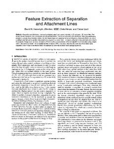
Medical Image

ModalityAcquisition

FMalgo_UPDATED

Format

MI Algorithm MRI

CT

PET

Name

MetaData

Method

Interactive

Anonymized

T2 Nifti MetaData implies Analyze Analyze excludes CT

Analyze

Model PAM

(a)

(b)

Figure 6. Updating FM views images. As multiple sources of variation are present within a service, several FMs are used where each FM focuses on a specific view of a service. As shown in [5], these FMs can then be used to check consistency between composed services and to facilitate their coherent configurations. 4.2.1

Updating FM views

In practice, the different FM views of a service are not independent. The workflow designer has to add constraints to enforce interactions between the FM views. In our example, we consider the following constraints: M IServiceconstraints = { (c1) F Mgrid .Kerberos ⇒ F Mproto .KDC (c2) F Mgrid .SSLAuth ⇔ F Mproto .SSL (c3) F MM Isupport .M RI ⇒ F Malgo .P AM (c4) F MM Isupport .CT ∨ F MM Isupport .SP EC ⇒ F Malgo .BAM (c5) F MM Isupport .Anonymized ⇒ F Mproto .HeaderEncoding (c6) ¬F Mgrid .GP U ∨ ¬F Malgo .Interactive (c7) F Malgo .Interactive ⇒ F Mgrid ..Linux (c8) F MM Isupport .DICOM ⇒ F Mproto .Rotation ∧ F Mproto .P AM (c9) F Malgo .Interactive ⇒ F Mproto .HeaderEncoding }

Determining the impact of these constraints on each FM view cannot be done manually or even automatically with current techniques and tools [10]. We rely on the corrective capabilities developed in Section 4.1 to perform the update of the different FM views. Using the slice operator, it simply consists in i) aggregating the four feature models into a single one (fmService) with constraints mapped on it, ii) invoking slice four times producing as much sliced FMs, the slicing criterion being respectively the features of each of the four feature models. As a result, Figure 6a and Figure 6b correspond to the sliced FM with respectively the features of the FMs F MM Isupport and F Malgo . The two other FMs are not impacted by the constraints mapped on fmService.

Managing Different FM Views

We illustrate the need to manage several FMs, possibly interrelated, using an example in the medical imaging domain. In this domain, medical imaging services (e.g., algorithms) are assembled to form complex processing chains (also called workflows). Variability affects different concerns or views of a medical imaging service. In Figure 5, the service is described through different views: information about the deployment on the grid, internal algorithms, the supported communication protocols and the type of handled medical

4.2.2

Supporting multiple perspectives

On the same example, the slice operator can be used to extract other views (or perspectives) of a service. In Figure 7, we capture expertises related to security features or to the medical imaging domain. Two slice operations are applied and compute two FM views, stored into fmViewMI 5

2012/3/2

FMgrid

FMalgo

GridDeployment

MI Algorithm Library Required

GridComputingNode

Method

Interactive

Matlab OS

Processor

Windows

FileSizeLimit GPU

Bits

Linux

CFL

Kerberos x32 Ubuntu

x64

Password

Non Grid

Model

PAM Affine

EMS

SSLAuth

Sc. Linux excludes MatLab

Sc. Linux

Linear

Atlas

Authentification

BAM

Rotation Scaling EMS implies Affine or Scaling

:grid :alg

Medical Imaging Registration Service

FMproto

:proto

TransferProtocol HTTPS

Medical Image Header Encoding

NetworkSecurity Crypto

HTTP

Format

ModalityAcquisition

SSL

PGP

Asymetric

FMMIsupport

:out

NetworkProtocol

MRI

CT

SPEC

PET

Symetric

Name

MetaData

Anonymized Analyze

DES TripleDES HeaderEncoding implies HTTPS

T2 T1 DICOM Nifti MetaData implies DICOM or Analyze Analyze excludes (CT and SPEC and T1)

KDC

Figure 5. Variability and concerns within a medical imaging service and 158 cross-tree constraints (CTCR2 =84%). The slicing technique significantly reduced the over approximation of the original architectural FM (from ≈ 1011 to ≈ 106 ). Variability in video surveillance. In the development of a video surveillance SPL, we represented the variability of the context and the variability of the software platform as two separated FMs [6]. 77 features and 108 configurations were present in the context FM while 51 features and 106 configurations were present in the software platform FM. The relationships between the two FMs were described as 39 rules (propositional constraints) relating features across models. Then, in line with specific requirements, we stepwise specialized the FM representing the context by removing some features, by modifying some feature groups, etc. After the specialization of the context FM, we needed to update the software platform FM. To do so, we aggregated the specialized context FM and the software platform FM together with rules. We used the slice operator on the aggregated FM by only including the set of features related to the software platform. We observed that from a specification of a context, the possible configurations in the software platform can be highly reduced. We applied the techniques on different scenarios: the average number of features to con-

and fmViewSecurity. The slicing criterion used to compute fmViewMI (resp. fmViewSecurity) contains features from the FMs F MM I , F Malgo and F Mgrid (resp. F MM I , F Mproto and F Mgrid ). The slice guarantees that all the interactions existing with other FM views are still enforced. 4.2.3

Practical applications

Reverse Engineering Architectural FMs. Besides the above application, the slicing technique was also extensively used in a tool-supported approach to reverse engineer software variability from an architectural perspective [3]. The proposed approach was evaluated when applied to FraSCAti, a large and highly configurable component and plugin-based system. Using the slicing technique an accurate view (i.e., an FM) of the software architecture was obtained. The idea was that the software architecture FM, originally produced by an extraction procedure, represents only an over approximation in terms of sets of valid configurations. Hence several sources of information were combined, namely software architecture, plugin dependencies and the correspondences between software elements and plugins. When combined through aggregation, slicing is used to update the view corresponding to the software architecture part. The aggregated FM resulting from the combination of different variability sources and the bidirectional mapping contains 92 features

2 CTCR

is the ratio of the number of features in the constraints to the number of features in the feature hierarchy.

fmViewMI MIService

fmViewSecurity MIService

MI Algorithm Library Required

Medical Image Method Model PAM

GPU

NetworkProtocol

Interactive

Authentification

ModalityAcquisition MRI

CT

Format

PET

Matlab

Name

NetworkSecurity

TransferProtocol HTTPS HTTP

Crypto

Asymetric

PGP

SSL

Symetric

T2 Nifti

Analyze DES

Analyze excludes CT

(a) Medical Image expert view

TripleDES KDC

Header Encoding

MetaData

Anonymized

Kerberos Password SSLAuth Anonymized implies HeaderEncoding HeaderEncoding implies HTTPS SSL ó SSLAuth Kerberos implies KDC

(b) Security expert view

Figure 7. Another decomposition strategy and set of FM views 6

2012/3/2

sider in the software platform FM was less than 104 (instead of 106 configurations). 4.3

feature (i.e., Nifti abstracts features NiftiI and NiftiII). Then, the comparison can be computed or the merge operator can be used as in Figure 8.

Reconciling Feature Models

4.3.2

When managing a set of FMs, the different stakeholders involved in the SPL development may have to put together very similar variability information but with a different structure. For example, in the medical imaging domain, different suppliers (scientists, research teams, companies, etc.) provide imaging services and may use different hierarchies, concepts, vocabulary, etc. when elaborating the FMs. 4.3.1

Besides the medical imaging domain, we also used the techniques described above for the reverse engineering of FraSCAti architectural FM. The architectural FM resulting from the automatic extraction (see Section 4.2.3) was compared with another architectural FM, this time manually designed by the software architect (SA) of FraSCAti. Unfortunately, the direct comparison yields to unexploitable results, mainly due to the difference of granularity (i.e., some features in one FM are not present in the other). Basic manual edits of FMs were unpractical as we needed to safely remove features involved in several constraints or that were in the middle of the hierarchy. The slicing operator was extensively applied to remove unnecessary details in both FMs. Once the FMs have been reconciled, the two FMs can be compared so that the differences between them can be identified. This encourages the SA to correct his initial model [3].

Technique and example

Let us consider two FMs, f mM I1 and f mM I2, in Figure 8. The two FMs differ. In particular, features Open, Proprietary, NiftiI, NiftiII are present in f mM I1 but not in f mM I2. Intuitively, more structure and details are modeled in f mM I1. As a result, a comparison (see Definition 3) or a merging (see Section 3.2) of the two FMs leads to counter intuitive results, i.e., the intersection of the two configuration sets is empty (see line 4 and 5 of the FAMILIAR script below). Looking at the two FMs, some configurations seem to correspond, for example, the valid configuration {M edicalImage, DICOM } of f mM I2 with the configuration {M edicalImage, Open, DICOM } of f mM I1. We thus need to reconcile (or align) the two FMs and allow an SPL practitioner to align in a coherent way information from f mM I1 and f mM I2.

4.4

fmMI1 MedicalImage

fmMI2

Nifti NiftiI

DICOM

SPI

4.4.1

MedicalImage

Proprietary

Nifti

GE

DICOM

Π MedicalImage, Nifti, DICOM, SPI, GE (fmMI1)

fmMI1Sliced 2

MedicalImage

∩ fmMI3 MedicalImage

Nifti DICOM

SPI

GE Nifti

DICOM

Realized-by property

An important property of an SPL is realizability, i.e., whether the set of products that the PL management decides to offer is fully covered by the set of products that the software platform allows building. In Figure 9, we want to ensure that for each valid selection/deselection of features of f mP L performed by a customer, there exists at least one corresponding software product described by f msof tware . The PL variability is documented using f mP L , the software variability is documented using another FM (see f msof tware ) and the two FMs are related through constraints (see mapSof tP L ). Note that the mapping between features of f mP L and f msof tware is not necessarily one-to-one. To this end we first reason about the relationship between f msof tware and f mP L . We compute f mG , the aggregation of f mP L and f msof tware and add the constraints mapSof tP L . In terms of FMs, the realizability property can be formally expressed (FP L the set of features of f mP L ):

SPI

NiftiII

1

Reasoning about Two Kinds of Variability

In SPL engineering, two kinds of variability are usually distinguished [22, 23]: software (or internal) variability, hidden from customers, as opposed to product line (PL) (or external) variability, visible to them. Software variability and PL variability can be seen as two concerns of an SPL. Metzger et al. proposed a formal and concise approach for separating PL variability and software variability and enabling automatic analysis [22]. The two concerns are modeled as two FMs and inter-related by constraints. The authors mention several properties that should be checked when reasoning about the two kinds of variability. We now revisit here the approach defended in [22] and show how the operators can be combined to support SoC in this context.

D EFINITION 3 (Kind of edits and Comparison). Let f and g be two FMs. f is a specialization of g if Jf K ⊂ JgK. f is a generalization of g if JgK ⊂ Jf K. f is a refactoring of g if JgK = Jf K. f is an arbitrary edit of g if f is neither a specialization, a generalization nor a refactoring of g. A comparison computes the relationship between two FMs.

Open

Practical application

SPI

Figure 8. Slicing (À) to reconcile FMs and allow, e.g., comparison or merging (Á) Using the slice operator, we simply remove features of f mM I1 i) that structure the feature model (i.e., features Open, Proprietary) and ii) that can be abstracted by a single

∀cp ∈ Jf mP L K, cp ∈ JΠFP L (f mG )K 7

(1) 2012/3/2

4.4.3

fmSoftware r

f1

Debit Card Payment

f2

Online Store

Payment Upon Voice

f3

Credit Card f4 Check of Payment Credit History

fmPL VP1

V1

Debit Card Payment

Reasoning about two concerns. We apply the techniques using the larger example described in [22]. We successfully retrieved the same results, but our approach is more efficient since we do not enumerate configurations/products as they do. Moreover, high-level operators (slice, aggregate, compare, merge) facilitate the reasoning realization and offer a systematic solution for SPL practitioners when understanding and maintaining the two FMs. It should be noted that the technique for updating views (see Section 6) can be applied in such contexts, for example, to remove dead features in the PL or software model. Reasoning about variability properties. In the development of video surveillance systems, a key issue is to ensure that, given a valid configuration of the context, a software configuration can always be obtained. This property is similar to the realized-by property and can be checked using the same techniques. We successfully scale for this case study, whereas it was clearly not the case with the enumerative technique proposed in [22].

V1 ó f1 V2 ó f2 V3 ó f3

Online Store

V2

Payment Upon Voice

V3

Check of Credit History

V2 => V3

Figure 9. Software and PL Variability (adapted from [22]) Intuitively, if the restriction of the PL features to Jf mG K is equivalent to the original Jf mP L K, the constraints mapSof tP L has no effect on the PL part of f mG and thus the realizability property holds. Otherwise some products cannot be realized in the platform. Equation 1 implies to check if f mP L is a refactoring (see Definition 3) of ΠFP L (f mG ). Using the aggregate, slice and merge diff operators, we can automatically check this property. First, we slice the aggregated FM f mG by only including FP L , the set of features of f mP L . The slice produces a new FM, denoted f mP LP rime . Formally: f mP LP rime = ΠFP L (f mG ) Then, we compare the resulting FM, f mP LP rime , with the original PL model, f mP L . If f mP LP rime is not a refactoring of f mP L , the realizability property is violated since some existing products of f mP L are removed in f mP LP rime and no product is added. Finally, we can compute the set of products that are in f mP L but not in f mP LP rime using the merge operator in diff mode. The merge operator produces f mP LDif f . Back to the example of Figure 9, we obtain that the realizability property does not hold and that three products proposed to customers cannot be realized by the platform:

5.

Towards Scalable Technique to Separate Concerns

Central to the support for SoC in feature modeling is the ability to decompose (i.e., slice) FMs. All applications described in the previous section make extensive use of the slicing technique. It is thus crucial to provide a scalable implementation of the slice operator. A syntactical technique is not adequate, especially in the presence of cross-tree constraints. A technique based on the enumeration of configurations is not scalable, since the number of configurations is exponential to the number of features. To avoid these limitations, we developed a dedicated technique that consists in first computing the propositional formula representing the projected (see Section 3.3) set of configurations. The computation of the propositional formula is essential for reasoning about the projected set of configurations but also for synthesizing the FM. As detailed in [4], propositional logic techniques [12, 29] can be applied to construct an FM (including its hierarchy, variability information and cross-tree constraints) from the formula. In this section, we focus on the computation of the propositional formula. We report on the practical limits of an implementation based on binary decision diagrams (BDDs). We describe a symbolic technique that outperforms a BDD-based implementation and that can efficiently decompose FMs with thousands of features. Propositional Formula Encoding. First, we describe the encoding of the projected set of configurations as propositional formula For a slicing F Mslice = Πf t1 ,f t2 ,...,f tn (F M ), the propositional formula φslice corresponding to F Mslice can be defined as follows: φslice ≡ ∃ f tx1 , f tx2 , . . . f txm0 φ

Jf mP L ⊕\ f mP LP rime K = Jf mP LDif f K = {{V 1, V 3, V 2, V P 1}, {V 1, V P 1}, {V 3, V P 1}}

Only the following two products can be realized: Jf mP L ⊕∩ f mP LP rime K = Jf mP LInter K = {{V 1, V 3, V P 1}, {V 2, V 3, V P 1}}

4.4.2

Practical applications

Non useful products

A product is useful if it is a possible realization of a PL member. As argued in [22], the list of non-useful products is a symptom of unused flexibility of the software platform. It can be on purpose, for example, justified by future marketing extensions. The usefulness property can be seen as the "symmetric" of the realized-by property. Formally, all products are useful if the following relation holds: ∀cp ∈ Jf msof tware K, cp ∈ JΠFsof tware (f mG )K

where f tx1 , f tx2 , . . . f txm0 ∈ (F \ Fslice ) = Fremoved . Intuitively, all occurrences of features that are not present in any configuration of F Mslice are removed by existential

Hence, similar techniques involving aggregate, slice and merge can be used to check the property. 8

2012/3/2

• The primary limit of the BDD-based implementation lies

quantification in φ. φslice is obtained from φ by existentially quantifying out variables in Fremoved .

in the difficulties to construct BDD from the original FM. In particular, the total number of features in the input FM should not be more than 2000 features, otherwise it is impossible to having a BDD-representation of the formula. It should be noted that whenever an FM can be represented as a BDD, φslice can be computed. Hence the encoding of φslice can scale up to 2000 features with a CTCR of 10, whatever the slicing criterion is ;

D EFINITION 4 (Existential Quantification). Let v be a Boolean variable occurring in φ. φ|v (resp. φ|v¯ ) is φ where variable v is assigned the value True (resp. False). Existential quantification is then defined as ∃v φ =def φ|v ∨ φ|v¯ . 5.1

BDD-based Implementation

In previous work [4], we rely on BDDs [11] to compute the propositional formula. A BDD is a compact representation of a Boolean function (e.g., a propositional formula). BDDs can be efficiently used to compute the propositional formula described above since computing the existential quantification can be performed in at most polynomial time with respect to the sizes of the BDDs involved [11]. Furthermore, BDDs can be used to synthesize an FM in polynomial time regarding the size of the BDD representing the input propositional formula [12]. A major drawback of BDDs is that finding an optimal variable ordering during BDD construction is NP-hard [11]. Some heuristics have been developed and successfully compile FMs to BDDs for a number of features up to 2000 [20]. The goal of our experiment was to determine the scalability of the BDD-based implementation w.r.t. the size of the input FMs (i.e., number of features) and the size of the slicing criterion (i.e., number of features to include). For the experiment, we reuse the heuristics (i.e., Pre-CL-MinSpan) developed in [20] to reduce the size of BDDs. For a first evaluation, we used several small and medium-sized FMs that were publicly available from SPLOT [21] repository as well as FMs from our case studies. We performed our experiments on more than 100 FMs, the bigger one having 290 features. We found that computing the slice is almost instantaneous in all cases. To go further, we randomly generated FMs with several hundreds of features. We varied i) the number of features, noted #f eatures, from 100 to 2000 features (the known practical limits of BDD) ; ii) CT CR from 10% to 100%. We used the publicly available procedure described in [21] to randomly generate the FMs. In each generated model, each type of mandatory, optional, Xor and Or-groups was added with equal probability. For each FM, we randomly generated a slicing criterion. We varied the percentage of features to slice between 100% (no existential quantification is performed) and 1% (almost all features are existentially quantified). The main results show that: • The synthesis of the feature diagram has practical limits (up to 800 features3 ). This limit also applies in our context. We observed that the slicing technique can scale even for an FM with 2000 features if the percentage of features to slice is ≤ 35%. The reason is that the size of a BDD will always be smaller or at least unchanged after existential quantification ;

5.2

SAT-based Implementation

She et al. proposed techniques to reverse engineer very large FMs (i.e., with more than 5000 features) [29]. As shown above BDDs do not scale for this order of complexity and therefore the slicing operator cannot process such FMs. She et al. adapted their previous techniques and now rely on satisfiability (SAT) solvers (rather than BDDs as in [12]). They reported that the use of SAT solvers is significantly more scalable. Hence a SAT-based implementation of slicing is an interesting perspective that motivates our work. We identify two main issues. First, the size of the formula exponentially increases when existential quantification is performed many times, i.e., the number of clauses doubles at each iteration. It may become an issue when the size of Fremoved is important, even for small FMs. Second, SAT solvers require a formula to be in conjunctive normal form (CNF). It is straightforward to translate the propositional formula of an FM into CNF. However, when existential quantification is performed, the resulting formula is not in CNF (see Definition 4). To tackle the first issue, we substitue each feature of Fremoved only in those clauses that contain the feature. More formally, let f t be a feature of Fremoved , φ a formula in CNF decomposed as follows: φ = p(f t, φ) ∧ c(f t, φ) where c(f t, φ) denotes the conjunction of the clauses that do not contain the feature f t and p(f t, φ) denotes the conjunction of the clauses that do contain the feature f t. The existential quantification of f t in φ produces a new formula φ0 defined as follows: φ0 = φ|f t ∨ φ|f¯t = (p(f t, φ)|f t ∨ p(f t, φ)f¯t ) ∧ c(f t, φ) Example. We consider f m1 of Figure 1a (see page 3). We slice f m1 using as slicing criterion all features except T and V (i.e., Fremoved = {T, V }). It should be noted that the existential quantification of T and V can performed in any order. In this example, we first perform the existential quantification of T, producing the following propositional formula: φ0f m1 = ((W ⇔ T rue ∧ V ⇒ T rue ∧ A ⇔ T rue) ∨ (W ⇔ F alse ∧ V ⇒ F alse ∧ A ⇔ F alse)) ∧ c(V, φ) ∧ T rue ∧ ¬F alse. Then we iterate by performing the existential quantification of V in φ0f m1 . We can observe that at each iteration the formula can be symbolically simplified in many ways. For instance, T cannot be evaluated to False in φ0f m1 and therefore the disjunctive clause can be removed. We can also observe that A ⇔ T rue ≡ T rue but we do not consider this kind of simplification since features included in the slicing criterion, like A, must not be removed. However we can sim-

3 Janota

et al. reported that the BDD-based algorithm proposed in [12] scales up only for FMs with 300/400 features [18], but did not use the heuristics proposed in [20]

9

2012/3/2

plify φ0f m1 considering that V ⇒ T rue ≡ T rue since V is included in the slicing criterion. An additional optimisation, related to symbolic simplification, is the order in which the features are existentially quantified. Indeed, we observe that some features are likely to be simplified. We use an heuristic that existentially quantifies in priority features that are at the bottom of the feature hierarchy. To tackle the second issue, we transform the resulting propositional formula into CNF at each iteration (i.e., for each existential quantification of a feature f t). It should be noted that we only need to consider the transformation of (p(f t, φ)|f t ∨ p(f t, φ)f¯t ) into CNF since c(f t, φ) is already in CNF. Generated FMs. For the evaluation of the technique, we used the same FMs as with the experiments conducted for the BDD-based implementation. We also generated FMs with 2000 ≥ #f eatures ≥ 10000 with the same parameters as previously described (10000 features is the practical limit admitted in the literature [10, 21, 32]). We first verified that the techniques described above are necessary since a naive substitution strategy that does not compute c(f t, φ) is not scalable (scalability issues are observed for #f eatures ≥ 50). Using our technique, we found that: i) computing the propositional formula is almost instantaneous for all FMs of SPLOT (less than one second, whatever the size of the slicing criterion is); ii) the SAT-based implementation scales for #f eatures ≤ 10000 whatever the size of the slicing criterion is; iii) the order in which the features are existentially quantified is of prior importance: we begin to observe scalability issues when quantifying first the features that are in top of the feature hierarchy for #f eatures ≥ 2000 ; iv) for very large FMs (#f eatures ≥ 5000), the computation time is inadequate for an interactive use of the slice operator (up to 20 minutes). Real world FMs. As stated early, automated extraction techniques now produce very large FMs from existing software systems. We applied our technique to three independent systems relating to the operating system domain (Linux, eCos, and FreeBSD). Linux and eCos have FMs whereas FreeBSD has not. She et al. reverse engineer the propositional formula of FreeBSD and develop techniques to interactively specify the hierarchy [29]. For the experiment, we directly applied the slicing technique on the formula of FreeBSD. It should be noted that, in this specific case, we cannot use the heuristic mentioned above since we do not have access to the hierarchy of FreeBSD. We randomly generated the order in which features are existentially quantified. The technique succeeded almost instantaneously (FreeBSD has 1203 features). We also succeeded on eCos that has over 1200 features. Finally, we applied our technique to the FM of Linux which exhibits 6300 features. Contrary to the results obtained from the two other operating systems or from the experimental study described above, we scaled only for less than 60% of features included in the slicing criterion (whereas this percentage drops to 1% in the other cases). In order to understand the reasons of this limitation, we need to

compare the experimental conditions of the generated FMs with the properties of the Linux FM. The Linux model contains very small percentages of mandatory features (5%), grouped features (3%) – Linux features are mostly optional (92%). whereas in each generated model, each type of mandatory, optional, Xor and Or-groups was added with equal probability (25%). We can make the assumption that the slice operator is dependent on certain shapes of FMs, and/or certain kinds of constraints. We need to understand the impact of FM properties regarding the scalability of the slice operator. As future work, we plan to characterize more precisely the lack of scalability w.r.t. the Linux FM and develop new heuristics or specific techniques.

6.

Comparison with Other Solutions

We now review existing approaches that have been developed to support SoC in FMs. We point out their relations to the SoC techniques that have been identified (see Figure 4) and illustrated by different case studies in Section 4. To this end, we rely on the numbers used in Figure 3, each corresponding to a case study. The general conclusion is that without the new capabilities brought by our solution (i.e., the combined use of composition and decomposition operators), some analysis and reasoning operations would not be made possible in the different case studies. Composition. A few works consider some forms of composition for FMs and suggest the use of a merge operator [7, 15, 27, 28]. An in-depth comparison of implementation approaches is performed in [2]. Our proposal goes further since we clarified the semantics of the merge and showed that the merge alone is not sufficient to realize complex management tasks in the case studies À and Â. It rather has to be combined with decomposition and reasoning mechanisms. Several approaches use several and interrelated FMs and views [15, 19, 22, 24, 35]. As shown, the aggregate operator combined with the slice can be used in such contexts to update the different views, to support multiple perspectives or to reason about properties of the FMs (see case studies À, Á, Â and Ã). In [26], the authors tackled the problem of mapping problem-space features into solutionspace features and proposed to use default logic. Our contributions rely on propositional logics and therefore are not applicable to this work. Thompson et al. proposed to specify a product family from n perspectives: one family-hierarchy per view such as software or hardware [31]. It is a form of SoC that is particularly needed in the case studies À or Á. A set-theoretic foundation is proposed: it can be expressed and realized using FMs and the presented techniques. Decomposition. Thüm et al. [32] presented an automated and scalable technique to characterize the kinds of edit between two FMs. An original property of the technique is that they distinguish abstract features from concrete features when reasoning. Abstract features are, in their work, nonleaf features. We consider this is the role of an SPL practitioner to explicitly determine which features are abstract 10

2012/3/2

7.

(as shown in the example of Section 4.3, abstract features are not necessary non-leaf features). Our technique is thus more general and realize the vision of [27] that makes the distinction between features that are of interest per se (i.e., that will influence the final product) and others. As we have shown, reasoning about the relationship of two FMs (and thus using the comparison operator developed in [32]) is inappropriate until FMs are not reconciled (see case studies À and Ã). From our experience, tool supported techniques, such as the safe removal of a feature by slicing, are not desirable but mandatory (i.e., basic manual edits of FMs are not sufficient) in this context. Recently, Thüm et al. [33] extend the work described in [32] and propose to make abstract features explicit in FMs. They show how a propositional formula can be retrieved describing the set of distinct "program variants", corresponding to combination of concrete features. Interestingly, Thüm et al. plan to apply their techniques to SPL testing. We see this work as an application of the slicing technique where all features but abstract features are part of the slicing criterion. Our technique for computing the propositional formula is similar to the technique described in [33]. In addition we developed an heuristic that determines the order in which the features are existentially quantified. We also applied to very large FMs and reported scalability results. In the context of feature-based configuration, techniques have been proposed to separate the configuration process in different steps or stages [13]. Our work is complementary since we propose techniques to decompose FMs. Hubaux et al. provide view mechanisms to decompose a large FM [17]. However they do not propose a comprehensive solution when dealing with cross-tree constraints. Furthermore we have shown that the decomposition of FMs has several other interesting applications beyond the support of multiple perspectives (see case studies À, Á, Â and Ã). Benavides et al. survey the literature of automated reasoning about FMs [10]. To the best of our knowledge, there is no existing work for correcting anomalies in FMs. Furthermore, existing approaches mentioned in [10] and discussed above either focus on composition or decomposition, but they do not try to combine the two mechanisms for supporting SoC in feature modeling. The "tyranny of the dominant decomposition” is a general issue for aspect-oriented approaches [30]. In [9], Batory et al. introduced multi-dimensional SoC where a dimension is a set of features addressing a particular concern. We can see a dimension as a slicing criterion. The approach of Batory et al. does not generate views but rather composes features along each dimension. It is thus complementary and can be used to produce parts of a system, being services (case study À), components (case study Á) or plugins (case study Ã). Rosenmüller et al. develop compositional support to manage different FMs, each focusing on a specific dimension [25]. They do not consider composition of FMs that introduce anomalies and do not propose automated decomposition (as needed in all case studies).

Threats to Validity

Threats to external validity are conditions that limit our ability to generalize the results of our operators and experiment to industrial practice. Our first concern is whether generated FMs or Linux FM used in the experiments (see Section 5) are representative of industrial usage. Our second concern is whether the composition and decomposition operators are expressive and intuitive enough to support activities of SPL practitioners. As summarized by Figure 4 and Figure 3, the operators have been applied to different domains for different purposes and by different people (external to our team). Moreover we identify several works in the literature that can benefit from the techniques (see Section 6). A first internal threat concerns the correctness of the operators implementation. In particular, the slice operator is supposed to guarantee that some semantic properties are preserved. Our implementation is currently checked by a comprehensive set of unit tests, complemented by cross-checked testing with other operations. For instance, we compared the formulas produced by the BDD-based and SAT-based implementation of the slice operator. We also manually verified a large number of slice examples. Besides we observed that randomly generated FMs may contain a lot of anomalies (e.g., dead features or wrong feature group). We used this opportunity to gain further confidence in our implementation and applied our slicing technique to automatically correct anomalies in generated FMs (see Section 4.1). We automatically checked that the original FM and the slice (i.e., corrected) FM were equivalent in terms of sets of configurations, that the slice FM did not contain any anomaly, and that the hierarchy conforms to the original FM.

8.

Conclusion

In this paper, we described how a set of complementary operators (aggregate, merge, slice) can be used to provide a powerful support for SoC in feature modeling. We showed how the operators can assist in tedious and error prone tasks such as automated correction of FM anomalies, update and extraction of FM views, reconciliation of FMs or reasoning about properties of FMs. The operators bring new capabilities to the FM users for supporting SoC in feature modeling and when we revisited and reimplemented existing approaches with them, we observed a better scalability. Both these new capabilities and scalability results enabled us to apply SoC in feature modeling to different domains (medical imaging, video surveillance) and for different purposes (scientific workflow design, variability modeling of context and software platform, reverse engineering). We also developed a technique to implement the slice operator that scales up to FMs with 10000 features in certain conditions. As future work, we plan to study practical usage and applicability of the proposed techniques. Acknowledgments. Dr. Acher’s work is supported by the IAP Programme, the Belgian Science Policy under the MoVES project, the FNRS, and an FSR grant, co-funded by Marie-Curie actions of the European Commission. 11

2012/3/2

References

[19] K. Kang, S. Kim, J. Lee, K. Kim, E. Shin, and M. Huh. Form: A feature-oriented reuse method with domain-specific reference architectures. Annals of Software Engineering, 5(1): 143–168, 1998.

[1] M. Acher. Managing Multiple Feature Models: Foundations, Language and Applications. PhD thesis, 2011. [2] M. Acher, P. Collet, P. Lahire, and R. France. Comparing approaches to implement feature model composition. In ECMFA’10, volume 6138 of LNCS, pages 3–19, 2010.

[20] M. Mendonca, A. Wasowski, K. Czarnecki, and D. Cowan. Efficient compilation techniques for large scale feature models. In GPCE’08, pages 13–22. ACM, 2008.

[3] M. Acher, A. Cleve, P. Collet, P. Merle, L. Duchien, and P. Lahire. Reverse engineering architectural feature models. In ECSA’11, volume 6903 of LNCS, pages 220–235, 2011.

[21] M. Mendonca, A. Wasowski, ˛ and K. Czarnecki. SAT-based analysis of feature models is easy. In SPLC’09, pages 231– 240. IEEE, 2009.

[4] M. Acher, P. Collet, P. Lahire, and R. France. Slicing feature models. In ASE’11, pages 424–427. IEEE, 2011.

[22] A. Metzger, K. Pohl, P. Heymans, P.-Y. Schobbens, and G. Saval. Disambiguating the documentation of variability in software product lines: A separation of concerns, formalization and automated analysis. In RE’07, pages 243–253, 2007.

[5] M. Acher, P. Collet, P. Lahire, A. Gaignard, R. France, and J. Montagnat. Composing multiple variability artifacts to assemble coherent workflows. Software Quality Journal (Special issue on Quality Engineering for SPLs), 2011.

[23] K. Pohl, G. Böckle, and F. J. van der Linden. Software Product Line Engineering: Foundations, Principles and Techniques. Springer-Verlag, 2005. ISBN 3540243720.

[6] M. Acher, P. Collet, P. Lahire, S. Moisan, and J.-P. Rigault. Modeling variability from requirements to runtime. In ICECCS’11, pages 77–86. IEEE, 2011.

[24] M.-O. Reiser and M. Weber. Multi-level feature trees: A pragmatic approach to managing highly complex product families. Requir. Eng., 12(2):57–75, 2007.

[7] V. Alves, R. Gheyi, T. Massoni, U. Kulesza, P. Borba, and C. Lucena. Refactoring product lines. In GPCE’06, pages 201–210. ACM, 2006.

[25] M. Rosenmüller, N. Siegmund, T. Thüm, and G. Saake. Multidimensional variability modeling. In VaMoS’11, pages 11–20. ACM, 2011.

[8] S. Apel and C. Kästner. An overview of feature-oriented software development. Journal of Object Technology (JOT), 8(5):49–84, July/August 2009.

[26] F. Sanen, E. Truyen, and W. Joosen. Mapping problem-space to solution-space features: a feature interaction approach. In GPCE ’09, pages 167–176. ACM, 2009.

[9] D. Batory, J. Liu, and J. N. Sarvela. Refinements and multidimensional separation of concerns. SIGSOFT Softw. Eng. Notes, 28:48–57, 2003.

[27] P.-Y. Schobbens, P. Heymans, J.-C. Trigaux, and Y. Bontemps. Generic semantics of feature diagrams. Comput. Netw., 51(2): 456–479, 2007.

[10] D. Benavides, S. Segura, and A. Ruiz-Cortes. Automated analysis of feature models 20 years later: a literature review. Information Systems, 35(6), 2010.

[28] S. Segura, D. Benavides, A. Ruiz-Cortés, and P. Trinidad. Automated merging of feature models using graph transformations. In GTTSE ’07, volume 5235 of LNCS, pages 489–505, 2008.

[11] K. S. Brace, R. L. Rudell, and R. E. Bryant. Efficient implementation of a bdd package. In DAC ’90: Design Automation Conference, pages 40–45. ACM, 1990.

[29] S. She, R. Lotufo, T. Berger, A. Wasowski, and K. Czarnecki. Reverse engineering feature models. In ICSE’11, pages 461– 470. ACM, 2011.

[12] K. Czarnecki and A. Wasowski. Feature diagrams and logics: There and back again. In SPLC’07, pages 23–34. IEEE, 2007. [13] K. Czarnecki, S. Helsen, and U. Eisenecker. Staged configuration through specialization and multilevel configuration of feature models. Software Process: Improvement and Practice, 10(2):143–169, 2005.

[30] P. Tarr, H. Ossher, W. Harrison, and S. M. Sutton, Jr. N degrees of separation: multi-dimensional separation of concerns. In ICSE’99, pages 107–119. ACM, 1999. [31] J. M. Thompson and M. P. E. Heimdahl. Structuring product family requirements for n-dimensional and hierarchical product lines. Requirements Engineering, 8(1):42–54, 2003.

[14] D. Dhungana, P. Grünbacher, R. Rabiser, and T. Neumayer. Structuring the modeling space and supporting evolution in software product line engineering. Journal of Systems and Software, 83(7):1108–1122, 2010.

[32] T. Thüm, D. Batory, and C. Kästner. Reasoning about edits to feature models. In ICSE’09, pages 254–264. ACM, 2009.

[15] H. Hartmann and T. Trew. Using feature diagrams with context variability to model multiple product lines for software supply chains. In SPLC’08, pages 12–21. IEEE, 2008.

[33] T. Thüm, C. Kästner, S. Erdweg, and N. Siegmund. Abstract features in feature modeling. In SPLC’11, pages 191–200. IEEE, Aug. 2011.

[16] H. Hartmann, T. Trew, and A. Matsinger. Supplier independent feature modelling. In SPLC’09, pages 191–200. IEEE, 2009.

[34] T. T. Tun and P. Heymans. Concerns and their separation in feature diagram languages - an informal survey. In International workshop SCALE@SPLC’09, pages 107–110, 2009.

[17] A. Hubaux, P. Heymans, P.-Y. Schobbens, D. Deridder, and E. Abbasi. Supporting multiple perspectives in feature-based configuration. Software and Systems Modeling, pages 1–23.

[35] T. T. Tun, Q. Boucher, A. Classen, A. Hubaux, and P. Heymans. Relating requirements and feature configurations: A systematic approach. In SPLC’09, pages 201–210. IEEE, 2009.

[18] M. Janota, V. Kuzina, and A. Wasowski. Model construction with external constraints: An interactive journey from semantics to syntax. In MODELS’08, volume 5301 of LNCS, pages 431–445, 2008.

[36] M. Weiser. Program slicing. In ICSE ’81, pages 439–449. IEEE, 1981.

12

2012/3/2