Proceedings of 2004 IEEE/RSJ International Conference on Intelligent Robots and Systems September 28 - October 2, 2004, Sendai, Japan
Sequential 3D-SLAM for mobile action planning Peter Kohlhepp, Paola Pozzo
Marcus Walther, Rüdiger Dillmann
Forschungszentrum Karlsruhe in der Helmholtz-Gemeinschaft, Institut für Angewandte Informatik Postfach 3640, D-76021 Karlsruhe
[email protected]
Universität Karlsruhe Institut für Rechnerentwurf und Fehlertoleranz Haid-und-Neu-Straße 7, D-76131 Karlsruhe
[email protected] processing. State spaces of increasing dimension, which arise inevitably during explorative mapping, are difficult to handle. Recently, Davison and Kita [5] proposed a frame work for adding and deleting components in a state vector, but we are aware of no results where EKF's have been practically used for the production of large and detailed 3D maps. For EKF, the statistical estimation problem should have a unique (uni-modal) solution, normally a Gaussian error distribution. But global position ambiguities arise when loops in large and complex environments need to be closed, inducing multi-modal pose density functions.
Abstract— Reliable mapping and self-localization in three dimensions while moving is essential to survey inaccessible work spaces or to inspect technical plants autonomously. Our solution to this 3D SLAM problem is novel in several respects. First, a new rotating laser-scanning setup is presented for acquiring point clouds and reducing them to surface patches in real time. Second, the SLAM algorithms work entirely on highly reduced, attributed surface models and in 3D. Third, we propose a novel system architecture of an Extended Kalman filter (EKF) for 3D position tracking, cooperating with a 3D range image understanding system for matching, aligning, and integrating overlapping range views. The system is demonstrated by an indoor exploration tour.
For ambiguous estimation problems, Markov models and Bayesian filters [25,26], in particular particle filters [19], Monte Carlo localization (MCL [25]) or the EM algorithm [20,24], are well studied. Starting from early work by Moravec and Elfes [21], the uniformly discretized pose space has been the prevailing data structure to implement Markov models. But grid maps do not well support on-line action planning, for example recognizing partially occluded objects, and they scale badly to three dimensions. Current work in 3D map making therefore typically takes a hybrid, multi-stage approach. Local position tracking as its backbone relies on scan matching in a 2D plane, which imposes some restrictions on the environment and cannot always recover six degrees of freedom. The subsequent global correction takes all available poses as a batch and often assumes planar pose transformations (xi,yi,θi), too. By applying the corrected 2D poses to the point data, a 3D model is finally obtained. Früh's city model building [9] using aerial views and MCL for global position correction, Liu's EM algorithm learning 3D models of indoor environments [20], and Thrun's underground mine mapping system [27] fall into this category. Except for the EM [20] creating a (basically predetermined) number of (infinite) planes, dense and rather unstructured point models mostly result.
Keywords - Simultaneous localization and mapping, 3DSLAM, laser scanner, range image, surface model, Extended Kalman Filter, uncertainty propagation
I.
INTRODUCTION
The inspection of thermally or chemically stressed parts in process plants, supported by infrared thermography, is an important application for future freely navigating mobile robots. Understanding and comparing the infrared images requires precise spatial alignment and the surface geometry to be known. Objects that are routinely examined must be recognized and relocated. These tasks require truly threedimensional environment maps. A similar problem arises in surveying and condition monitoring hardly accessible environments, e.g. mines [27]. In such areas of poor illumination, active optical sensors (laser scanners) lend themselves for environment capture despite their higher cost and lower resolution as compared to video cameras. The map should show up-to-date objects and obstacles of a work space that may gradually change. Representation and level of detail must be tailored to on-line planning algorithms. Therefore it seems no vital option to just import a CAD plant model born long ago, such as one generated by reverse engineering tools [1,3,7] and for a different purpose. Inspection robots should rather themselves build the map best suited to their mission. When exploring the work space, many local views must be localized in the map. Thus they face a simultaneous localization and mapping problem (SLAM) in 3D. Positions and map are both subject to a growing uncertainty.
Our approach differs in several respects. Most importantly, all SLAM steps use and produce highly reduced surface models [17,18] whose size remains bounded by the geometric complexity of the mapped space. Their geometric-topological structure is useful for action planning. Second, full 3D information is always exploited by surface matching of adjacent scene views. Third, global pose corrections are propagated on-line in an elastic graph with a bounded number of elastic sub-maps. Corrections may ensue from new feature correspondences (cycle closing) found in a limited area of previously mapped space, where the area size depends on the accumulated uncertainty. A rating function on propagated surface correspondences takes the role of the pose density function in our case.
Statistical methods, in particular recursive filters like the Extended Kalman filter (EKF) have been extensively used in this area [2,5,6,10,22]. EKF observe positions from complementary noisy sensor signals (wheel encoders, camera image features..) and are ideally suited for real time
0-7803-8463-6/04/$20.00 ©2004 IEEE
722
the accuracy of existing ones improves by redundant measurements.
In this paper we focus on the 'local' aspects. We achieve sequential surface capture of the work space by using a commercial 2D laser scanner and a new rotating sensor arrangement (section II). The localization and mapping combines an Extended Kalman filter for coarse pose tracking with a 3D range image understanding system [12], and propagates the uncertainties of both (sections III and IV). II.
REAL TIME DATA CAPTURE AND SURFACE SEGMENTATION
The robot equipped with laser line scanner(s) has to map an unknown workspace so as to use the map at any moment for mission planning. When no external position reference like GPS is applicable, the vehicle must determine its position in the map from well known visual features, or determine the relative pose of new features from its known current position in the map. Indeed both happens alternatingly. Key requirements for reliable pose estimation and map making are redundancy of sensed features, and a good vehicle overview of both the ahead areas and the lateral work space (ideally omni-directional view). In order to meet these requirements, the scanning plane must be tiltable independently of the driving direction. The market of 3D laser scanners with two independent axes of rotation remains narrow, and the few commercial devices are specialized in the CAD modeling of large plants [1, 3].
Figure 1. Sensor geometry (top), and rotating SICK laser scanner RoSi on the mobile platform Odete (bottom)
This approach requires to reduce or segment each range view in real time, but how to define these units of information ? In the case of a 2D laser scanner or a line camera it seems obvious to take each scan line as a range view. Indeed there exist a few algorithms that extend scan lines to surface patches in real time, notably the ones developed for polyhedral scenes by Jiang and Bunke in 1994 and generalized some years later to second order surfaces [13,14]. As the surface patches grow from line or 2nd degree polynomial segments in single scan lines, so to say from degenerate 'patches', the estimation of their normal vectors must be sensitive to uncertainties in the direction across scan lines, where precisely the growing uncertainty of the underlying vehicle position comes into play. For this reason we voted for a region based segmentation as a more robust alternative. It requires however to package consecutive scan lines into images. In case of the rotating scanner RoSi the point set taken during half a resolution yields a complete range image, after which the information repeats. Consecutive images tend to show a large amount of overlap.
A new sensor geometry was developed at the Karlsruhe University institute for computer design and fault tolerance. It permits a conventional 2D laser scanner (SICK LMS) to freely rotate around its optical axis, and is named the Rotating SICK laser scanner RoSi [23]. Power supply and data communication are made of gold sliprings. Its assembly on a mobile platform Odete is shown in figure 1. With the SICK LMS scanner a spherical cap with opening angle of approximately 100° in front of the vehicle is captured; in case of a 180° sector it would be a hemisphere. Owing to the rotation of the scan lines no orientations are preferred, but objects in the center receive the highest resolution and at the border of the view field the lowest. The concept optimally supports control of the focus of attention, obstacle recognition, and path planning of a vehicle. Real time mapping aimed at action planning requires also to reduce points to surface features or even symbolic features, while growing partial views into larger models. Procedures known from reverse engineering align and merge partial views early, at the low level of point clouds or triangle networks, and generate a surface model at the very end [1,7] (Eearly fusion, Late compression). Such a batch procedure will basically not transfer to real time operation, because it would have to re-generate a map better suited to action planning time and again, from a monotonically growing point model.
An enhanced split-and-merge procedure (Tree of Pyramid [16]) was applied to extract maximal connected and geometrically homogeneous surface patches. The entire image is recursively split into regions at points which locally maximize some criteria of non-homogeneity, such as points with maximum distance from a reference surface defined on the region border, or points with a high strength of crease or curvature edges. The partitioning is continued until geometrically homogeneous seed regions (solid facets) evolve. Adjacent facets are then merged in another order to form larger surface patches. Just like polygonshaped facets, also single range pixels may be assigned to a neighboring facet. Regions with no valid scan points or very low point density, likewise regions no longer divisible but still inhomogenous (transparent facets) do not form new surface patches, but leave gaps to be partially filled later by neighboring surfaces. Thus a mosaic of patches linked by relations develops, but no connected overall surface.
We apply an Early compression, Late fusion approach [17,18]: each range view is immediately reduced to surface patches and then merged with the current surface map. Point data from earlier steps will be lost. Thus, the map size grows with the geometrical complexity of the mapped work space only, not with the time spent surveying. It stops growing when no more new features are mapped and only
723
Fig. 2 shows on top a dense RoSi range image. Each half revolution contains 150-200 scan lines, depending on the angular velocity that the scan rate permits. This gives an angular resolution of approximately 2°. Each scan line has 401 points, according to the 100° opening angle of the SICK sensor and its angular resolution of 0.25°. A reduction to mostly planar surface patches is shown on the bottom. The complexity of segmentation is N log(N) in the number of pixels N, but almost linear in practice. Average running times of 2-3 seconds for 60-80000 pixel images were measured on a 2.2GHz P4 PC, which almost matches the RoSi acquisition speed (1-8 seconds per revolution).
v u Rectangle
Linear scanning
v u Möbius band
Rotating around the optical axis
Figure 3. Sensor geometry and resulting parameter space topology
For example the RoSi setup, where u∈[0,π] symbolizes the rotation angle of a scan line during half a revolution, and v∈[0,100°] the angle of deflection of each point from the optical axis, leads to a rectangle with two opposite sides glued together in reverse orientation (the scan lines for umin=0 and umax=π), forming a twisted cylinder mantle or Moebius band, see figure 3.
All surface patches have outer and inner 3D boundary polygons, center of gravity, mean direction vector, curvature distribution and planar approximation. Relations between patches, and additional numerical attributes are also calculated, e.g. the included area per patch, a principal component shape factor, and the degree of occlusion by other patches. From this information the free, occupied, or unknown space are readily inferred, and 'invariant' surfaces such as the floor can be identified and tracked (an example is mentioned in section V). The level of detail of the surface model is controllable to efficiently answer queries such as the direction and distance of the closest obstacle.
Thus, for a pixel (u, v) not only (u±1, v±1) but also (umin, v) and (umax, vmax -v ±1) are neighbors for any v. This is considered in the 8-neighbourhood and local mask operator definitions for picture smoothing or normal vector estimation. Since the Moebius band is a non-orientable manifold - there is no 'left of' or 'right of a region' as in a plane - well-known procedures for extracting closed region boundaries had to be adapted, too: contour following has to keep track of all crossings of the vmax border by parameter coordinates, flipping the contour orientation each time.
Like most range segmentation algorithms, Tree of Pyramid also requires parameterized range images ordered by scan lines. This 2D ordering is strongly exploited to determine neighborhood, connectivity or proximity of regions, and for many purposes it substitutes the Euclidean distance. By this resort to 2D image processing techniques, real time segmentation of 3D point clouds becomes feasible. A rectangular parameter space [umin, umax]× [vmin, vmax] is mostly assumed. Other sensor geometries however result in a different topologies of the parameter space (fig. 3).
Further important adjustments concern the expected scanning density in the range image which now strongly depends on the pixel position. Density approaches infinity in the image center. And, due to vehicle motion, the noise level of the 3D points is not uniform but keeps increasing from the first to the last scan line. III.
SEQUENTIAL IMAGE REGISTRATION AND FUSION
From a range image sequence the observer trajectory can be determined by matching and aligning consecutive range images without any prior knowledge of vehicle positions. But in practice it seems to work reliably only if the overlap, or ratio of redundantly seen features in consecutive images is high (empirical figure: ≈ 80%, see section V), and if the work space has distinctive structures. Otherwise, the running times become unforeseeable, or, since the correspondence and pose estimating algorithm must react any-time, the vehicle will lose its correct pose after a few steps, and will fail to provide a consistent map. On the other hand, we recently showed that even very crude motion assumptions tremendously improved the reliability of pose tracking in range image sequences [18]. Statistically sound results are expected from vehicle sensors like wheel encoders, gyros, inclination, or acceleration sensors, when quantitative error models are supplied. Different signals are weighted by their uncertainty and fused in an Extended Kalman filter which yields an overall position estimate and its covariance matrix. Still, the occasional correction by redundant optical feature measurements
Figure 2. Top: range image covering one half revolution of RoSi (the first scan line is highlighted), bottom: coarse surface reduction.
724
remains indispensable in order to reduce uncertainty. Mostly, such a correction would be done within the EKF framework, by aggregating the vehicle state and the visual features in a joint state vector [2,4,6,10].
From each feature correspondence, the rotation and translation minimizing the mean registration error are estimated using the algorithm by Horn [11,17]. Correspondence and pose are then iteratively improved on the middle level, maximizing the location-dependent overall similarity between the surface models. The achieved boundary overlap is assessed here, too. Alternatingly, the correspondence is optimally grown or shrunk for fixed pose, and then the pose re-adjusted to the new correspondence, reminiscent of the Expectation Maximization approach [20]. On the top layer, an evolutionary algorithm can escape local minima by mutation and recombination of correspondence relations; it is however not part of the real-time system.
Whatever the cause and the degree of discrepancy between estimated and true vehicle pose, its correction is some rigid transformation (rotation and translation) which should simultaneously align certain visible features in the map with corresponding features of the range view at the current uncertain position, in the best possible way. This assuming a known scanning geometry, and stationary landmark features available. But a Kalman filter does not address this orthogonality constraint when estimating poses; at best, the transformations may approach orthogonality asymptotically. Also, an EKF does not seem appropriate to manage a huge and growing 'state vector' made from all the features of an exploratively mapped work space. Therefore we decide for another and, as we believe, novel co-operation between an EKF and a 3D range image understanding system. It is represented as a data flow diagram in figure 4.
After alignment, the partial surface models may be merged as attributed graphs. A subtle part of the algorithm merging the partially redundant patches has been described in [8]: it implements a boolean operation (union / difference) on noisy 3D boundary polygons, based on a threshold value of their Haussdorff distances. The merging operation returns a degree of confidence in the soundness of the underlying feature correspondence and transformation.
1. The vehicle pose with three position and four orientation components is continuously being estimated from signals of wheel encoders and inclination sensors by means of the EKF. The filter models the inclinations of the terrain as unknown disturbances, see section IV. The initial pose is arbitrary; we define the first vehicle location as the origin of the world (map) coordinate system.
3. Each time RoSi (lower block in figure 4) supplies a new segmented range view, a running estimate of its observer pose is recalled from the EKF as a location transformation xnav = (p, Q) where p denotes a translation vector and Q a rotation w.r.t. the map origin. By using the current uncertainty (covariance matrix CX,nav) of the vehicle sensors, the range image processing system restricts its search area for corresponding surface features given by the location-invariant constraints. To achieve this, a new locationuncertain similarity measure based on Mahalanobis distance is defined between corresponding feature candidates vM in the map M and vS in the current partial model S:
2. The environmental map with a 'state vector' of variable dimension is managed by a 3D range image understanding system alone. Its major task is to repeatedly align and merge new range views. This basic cycle of position estimation and map generation is implemented in three layers. The lowest one looks for the best surface assignments, allowing for partial occlusion and also segmentation errors. Feature matching uses location invariant similarity measures between surfaces and relations of two or more surfaces, e.g. the similarity of the scalar triple products or spin representations [15] is a criterion. 3Dpose estimation from navigation sensors
Vehicle sensors Distance & orientation Roll &Pitch (inclination)
3D terrain model Disturbance
Rotating laser scanner Distance Deflection rotation angles
Result Result m map ap
Surface model fusion Re-Initialization xmap, C
x,map
Search space
Pose estimate xnav =(p, Q)
Pose-dependent
Uncertainty
similarity Pose-uncertain
x,nav
Pose-invariant
Pose estimate Evolutionary algorithm Iterative optim optimization Correspondence Correspondenceand pose estimation
Packaging
Ordered uncertain point clouds
Segmentation
1
(1)
Example 1 - Rotation Estimation: Let mi := (mi,x, mi,y, mi,z)T and si := (si,x, si,y, si,z)T for i =1..N corresponding vector features from the map M and the current range view S, respectively. The rotation by the Horn algorithm best aligning mi with si in the least-squares sense and written as a quaternion, is known to be the eigenvector Q to the smallest eigenvalue of the symmetrical 4×4 matrix A [11]:
Real-time Surface reduction Coordinate transformation
)
Direction or axis vectors, or connecting vectors between center points of totally visible patches serve as feature vectors. During pose tracking a unique feature correspondence mostly remains that fulfils both the locationindependent and location-uncertain constraints. The pose transformation xmap=(pmap,Qmap) estimated thereof has its own uncertainty CX,map. The calculation scheme and the associated propagation scheme of the covariance matrices is summarized in fig. 5. It starts from scan points corrupted by independent measurement noise but containing also a common term of vehicle pose uncertainty, then proceeding to surface estimation from points, estimating their pose relative to the corresponding mapped features, and finally aligning and merging the surface features.
understanding
Extended Kalman Filter
−1
( vˆ M := Q(vM ) + p denotes transformed map features).
3D Range image
Kalman gain matrix
C
(
sim nav (v M , v S ) := exp − vˆ TM ⋅ C x ,nav ⋅ v S ∈ [0 , 1]
2
Segmentedrange entedrangeviews
Figure 4. Block diagram for real time localization and mapping in 3D
725
N
A=
∑
S Ti ⋅ S i ,
Surface Estimation
(2)
...
Transform SKS→WKS
CmS
Cx,nav
CmS
b = (b1 , L, bN )T , bi = si − Q ∗ mi ∗ Q- 1 , ni
Cx,map
For any successful pose estimation, xmap and its uncertainty CX,map are sent back to the EKF to re-initialize its estimation, xnav and CX,nav, respectively. Both subsystems work at different time scales; approximately every 50-100 milliseconds for the EKF and every 2-3 seconds for the range image processing system.
In many cases, the uncertainty propagation from surface features to transformation parameters or transformed features are straightforward. In example 1 or similar cases, however, the perturbation of the eigenvectors of symmetrical matrices is needed. If A∈ℜn×n is a symmetrical matrix, there exists an orthonormal matrix H such that
IV. STATE MODEL FOR VEHICLE LOCALIZATION WITH NAVIGATION SENSORS
H −1 ⋅ A ⋅ H = diag (λ1 ,K , λn )
The vehicle trajectory has been modeled as a nonlinear discrete-time state model, following work of Davison and Kita for navigating on undulating terrain [4]. We give the details found necessary to implement the filter. The state is observed by wheel encoders for two drive wheels yielding distance and change of vehicle orientation, and by two inclinometers in the current longitudinal and lateral vehicle directions. The state x = (p, Q) covers translation and rotation of the vehicle coordinate system FKS with respect to the world coordinate system WKS. The rotation is represented by a quaternion Q with the corresponding rotation matrix R written as orthonormal column vectors
where λ1 ≤ λ2 ≤ ... ≤ λn are the eigenvalues of A sorted in increasing order. I.e. λ1 is the smallest eigenvalue, and its eigenvector x is H's first column vector. Here the following result by Weng et al. [28] is used: If λ1 is a simple eigenvalue (λ1