Oct 13, 2009 - Roman Garnet, Michael A. Osborne, Steven Reece, and Stephen J. Roberts. Robotics Research Group. Department of Engineering Science.
Sequential Bayesian Prediction in the Presence of Changepoints and Faults Technical Report PARG-09-01 Roman Garnet, Michael A. Osborne, Steven Reece, and Stephen J. Roberts
Robotics Research Group Department of Engineering Science University of Oxford October 13, 2009
Abstract
i.i.d. observations from an associated probability distribution. The problem of changepoints in dependent processes has received less attention. Both Bayesian (Carlin et al., 1992; Ray & Tsay, 2002) and nonBayesian (Muller, 1992; Horv´ ath & Kokoszka, 1997) solutions do exist, although they focus on retrospective changepoint detection alone; their simple dependent models are not employed for the purposes of prediction. Sequential and dependent changepoint detection has been performed (Fearnhead & Liu, 2007) only for a limited set of changepoint models. Fault detection, diagnosis and removal is an important application area for sequential time-series prediction in the presence of changepoints. Venkatasubramanian et al. (Venkatasubramanian et al., 2003) classify fault recognition algorithms into three broad categories: quantitative model-based methods, qualitative methods and process history based methods. Particularly related to our work are the quantitative methods that employ recursive state estimators. The Kalman filter is commonly used to monitor innovation processes and prediction error (Willsky, 1976; Basseville, 1988). Banks of Kalman filters have also been applied to fault recognition, where each filter typically corresponds to a specific fault mode (Kobayashi & Simon, 2003; Aggarwal et al., 2004; Reece et al., 2009a). Gaussian Processes are a natural generalisation of the Kalman filter and, recently, fault detection has also been studied using GPs (Garnett et al., 2009; Reece et al., 2009b). We introduce a fully Bayesian framework for performing sequential time-series prediction in the presence of changepoints. We introduce classes of nonstationary covariance functions to be used in Gaussian process inference for modelling functions with changepoints. We also consider cases in which these changepoints represent a change not in the variable of interest, but instead a change in the function determining our observations of it, as is the case for sensor faults. In such contexts, the position of a particular changepoint becomes a hyperparameter of the model. We proceed as usual when making predictions and evaluate the full marginal predictive distribution. If the locations of changepoints in the data are of interest, we estimate the full posterior distribution of the related hyperparameters given the data. The result is a robust time-series prediction algorithm that makes well-informed predictions even in the presence of sudden changes in the data. If desired, the algorithm additionally performs changepoint and fault detection as a natural byproduct of the prediction process. The remainder of this paper is arranged as follows. In the next section, we briefly introduce Gaussian pro-
We introduce a new sequential algorithm for making robust predictions in the presence of changepoints. Unlike previous approaches, which focus on the problem of detecting and locating changepoints, our algorithm focuses on the problem of making predictions even when such changes might be present. We introduce nonstationary covariance functions to be used in Gaussian process prediction that model such changes, then proceed to demonstrate how to effectively manage the hyperparameters associated with those covariance functions. We further introduce covariance functions to be used in situations where our observation model undergoes changes, as is the case for sensor faults. By using Bayesian quadrature, we can integrate out the hyperparameters, allowing us to calculate the full marginal predictive distribution. Furthermore, if desired, the posterior distribution over putative changepoint locations can be calculated as a natural byproduct of our prediction algorithm.
1
Introduction
We consider the problem of performing time-series prediction in the face of abrupt changes to the properties of the variable of interest. For example, a data stream might undergo a sudden shift in its mean, variance, or characteristic input scale; a periodic signal might have a change in period, amplitude, or phase; or a signal might undergo a change so drastic that its behavior after a particular point in time is completely independent of what happened before. We also consider cases in which our observations of the variable undergo such changes, even if the variable itself does not; as might occur during a sensor fault. A robust prediction algorithm must be able to make accurate predictions even under such unfavorable conditions. The problem of detecting and locating abrupt changes in data sequences has been studied under the name changepoint detection for decades. A large number of methods have been proposed for this problem; see (Basseville & Nikiforov, 1993; Brodsky & Darkhovsky, 1993; Csorgo & Horvath, 1997; Chen & Gupta, 2000) and the references therein for more information. Relatively few algorithms perform prediction simultaneously with changepoint detection, although sequential Bayesian methods do exist for this problem (Chernoff & Zacks, 1964; Adams & MacKay, 2007). However, these methods—and most methods for changepoint detection in general—make the assumption that the data stream can be segmented into disjoint sequences, such that in each segment the data represent 1
cesses and then discuss the marginalisation of hyperparameters using Bayesian Monte Carlo numerical integration in Section 3. A similar technique is presented to produce posterior distributions and their means for any hyperparameters of interest. In Section 4 we introduce classes of nonstationary covariance functions to model functions with changepoints or faults. In Section 5 we provide a brief expository example of our algorithm. Finally, we provide results demonstrating the ability of our model to make robust predictions and locate changepoints effectively.
2
Our GP distribution is specified by the values of various hyperparameters collectively denoted θ. These hyperparameters specify the mean function, as well as parameters required by the covariance function: input and output scales, amplitudes, periods, etc., as needed. Note that we typically do not receive observations of y directly, but rather of noise-corrupted versions z of y. We consider only the Gaussian observation likelihood p( z | y, θ, I ). In particular, we typically assume independent Gaussian noise contributions of a fixed variance η 2 . This noise variance effectively becomes another hyperparameter of our model and, as such, will be incorporated into θ. To proceed, we define
Gaussian process prediction
V (x1 , x2 ; θ) , K(x1 , x2 ; θ) + η 2 δ(x1 − x2 ) ,
Gaussian processes (GPs) offer a powerful method to perform Bayesian inference about functions (Rasmussen & Williams, 2006). A GP is defined as a distribution over the functions X → R such that the distribution over the possible function values on any finite set F ⊂ X is multivariate Gaussian. Consider a function y(x). The prior distribution over the values of this function is completely specified by a mean function µ(·) and a positive-definite covariance function K(·, ·). Given these, the distribution of the values of the function at a set of n inputs, x, is
(1)
where δ(·) is the Kronecker delta function. Of course, in the noiseless case, z = y and V (x1 , x2 ; θ) = K(x1 , x2 ; θ). We define the set of observations available to us as (xd , z d ). Taking these observations, I, and θ as given, we are able to analytically derive our predictive equations for the vector of function values y ⋆ at inputs x⋆ p(y ⋆ |z d , θ, I) � = N y ⋆ ; m(y˚⋆ | z d , θ, I) , C(y˚⋆ | z d , θ, I) , (2)
p( y | I ) , N(y; µ(x), K(x, x)) 1 ,p n (2π) det K(x, x) � � 1 exp − (y − µ(x))T K(x, x)−1 (y − µ(x)) , 2
where we have1
m(y˚⋆ | z d , θ, I) = µ(x⋆ ; θ) + K(x⋆ , xd ; θ)V(xd , xd ; θ)−1 (z d − µ(xd ; θ)) C(y˚⋆ | z d , θ, I) =
where I is the context, containing all background knowledge pertinent to the problem of inference at hand. We will typically incorporate knowledge of relevant functional inputs x into I for notational convenience. The prior mean function is chosen as appropriate for the problem at hand (often a constant), and the covariance function is chosen to reflect any prior knowledge about the structure of the function of interest, for example periodicity or a specific amount of differentiability. A large number of covariance functions exists, and appropriate covariance functions can be constructed for a wide variety of problems (Rasmussen & Williams, 2006). For this reason, GPs are ideally suited for both linear and nonlinear time-series prediction problems with complex behavior. In the context of this paper, we will take y to be a potentially dependent dynamic process, such that X contains a time dimension. Note that our approach considers functions of continuous time; we have no need to discretise our observations into time steps.
K(x⋆ , x⋆ ; θ) − K(x⋆ , xd ; θ)V(xd , xd ; θ)−1 K(xd , x⋆ ; θ) . We will also make use of the condensed notation my|d (x⋆ ) , m(y˚⋆ | y d , , I) and Cy|d (x⋆ ) , C(y˚⋆ | y d , I). We use the sequential formulation of a GP given by (Osborne et al., 2008) to perform sequential prediction using a moving window. After each new observation, we use rank-one updates to the covariance matrix to efficiently update our predictions in light of the new information received. We efficiently remove the trailing edge of the window using a similar rankone “downdate.” The computational savings made by these choices mean our algorithm can be feasibly run on-line. 1 Here the ring accent is used to denote a random variable e.g. ˚ a = a is the proposition that variable ˚ a takes the particular value a.
2
3 3.1
Marginalisation
likelihood for each sample. Of course, this sampling is necessarily sparse in hyperparameter space. For θ far from our samples, θs , we are uncertain about the values of the two terms in our integrand: the predictions
Posterior predictive distribution
Of course, we can rarely be certain about θ a priori, so we proceed in the Bayesian fashion and marginalise our hyperparameters when necessary. We will assume our hyperparameter space has finite dimension and write φe for the value of the e th hyperparameter in θ. φi,e is used for the value of the e t h hyperparameter in θi . For each hyperparameter we take an independent prior distribution such that Y p( θ | I ) , p( φe | I ) .
˚ q (θ) , p( y ⋆ | z d , θ, I ) , and the likelihoods ˚ r (θ) , p( z d | θ, I ) . It is important to note that the function q evaluated at a point θ returns a function (a predictive distribution for y ⋆ ), whereas the function r evaluated at a point θ returns a scalar (a marginal likelihood). To estimate (7), BQ begins by assigning GP priors to both q and r. Given our (noiseless) observations of these functions, q s , q(θ s ) and rs , r(θ s ), the GPs allow us to perform inference about the function values at any other point. Because integration is a projection, and variables over which we have a multivariate Gaussian distribution are joint Gaussian with any affine transformation of those variables, our GP priors then allow us to use our samples of the integrand to perform inference about the integrals. We define our unknown variable R q(θ) r(θ) p(θ|I) dθ . ˚ ̺ , p(y ⋆ |z d , I) = R r(θ) p(θ|I) dθ
e
For any real hyperparameter φe , we take a Gaussian prior � (3) p( φe | I ) = N φe ; νe , λe 2 ;
if our hyperparameter is restricted to the positive reals, we instead assign a Gaussian distribution to its logarithm. For a hyperparameter φe known only to lie between two bounds le and ue , we take the uniform distribution over that region, p( φe | I ) =
⊓(φe ; le , ue ) , ∆e
(4)
where ∆e , ue − le and ⊓(θ; l, u) is used to denote the rectangular function ( 1 (le < φe < ue ) ⊓(φe ; le , ue ) , . (5) 0 (otherwise)
and
m(˚ ̺ | q s , r, I) , in order to proceed as
Occasionally we may also want to consider a discrete hyperparameter φe . In this case we will take the uniform prior 1 , (6) P ( φe | I ) = ∆e where ∆e is here defined as the number of discrete values the hyperparameter can take. Our hyperparameters must then be marginalised as R p(y ⋆ |z d , θ, I) p(z d |θ, I) p(θ|I) dθ R . p(y ⋆ |z d , I) = p(z d |θ, I) p(θ|I) dθ (7) Although these required integrals are non-analytic, we can efficiently approximate them by use of Bayesian Quadrature (O’Hagan, 1991) (BQ) techniques. As with any method of quadrature, we require a set of samples of our integrand. Following (Osborne et al., 2008), we take a grid of hyperparameter samples θs , ×e φu,e , where φu,e is a column vector of unique samples for the e th hyperparameter and × is the Cartesian product. We thus have a different mean, covariance and
R
mq|s (θ) r(θ) p(θ|I) dθ R , r(θ) p(θ|I) dθ
p( y ⋆ | q s , r s , z d , I ) ZZZ = p( y ⋆ | q, r, z d , I ) p( ̺ | q, r, I ) p( q | q s , I ) p( r | r s , I ) d̺ dq dr =
=
ZZZ Z
̺ δ(̺ − ˚ ̺) N q; mq|s , Cq|s
�
� N r; mr|s , Cr|s d̺ dq dr
� m(˚ ̺ | q s , r, I) N r; mr|s , Cr|s dr .
Here our integration again becomes non-analytic. As a consequence, we take a maximum a posteriori (MAP) approximation for� r, which approximates � N r; mr|s , Cr|s as δ r − mr|s . This gives us Z p( y ⋆ | q s , rs , z d , I ) ∝ ∼ mq|s (θ) mr|s (θ) p(θ|I) dθ. 3
3.2
We now take the independent product Gaussian covariance function for our GPs over both q and r Y K(θi , θj ) , Ke (φi,e , φj,e ) e (8) � Ke (φi,e , φj,e ) , N φi,e ; φj,e , we2 ,
We can also use BQ to estimate the posterior distribution for hyperparameter φf (which could, in general, also represent a set of hyperparameters) by marginalising over all other hyperparameters φ−f R p(z d |θ, I) p(θ|I) dφ−f p(φf |z d , I) = R . p(z d |θ, I) p(θ|I) dθ
and so, defining
Ne (φi,e , φj,e ) , Z Ke (φi,e , φ∗,e ) p(φ∗,e |I) Ke (φ∗,e , φj,e ) dφ∗,e ,
Here we can again take a GP for r and use it to perform inference about ˚ ρ , p(φf |z d , I). We define R r(θ) p(θ|I) dφ−f , m(˚ ρ | r, I) = R r(θ) p(θ|I) dθ
we have � � � � 2 �� λ +w2 ν φi,e ; e , e 2 e Ne (φi,e , φj,e ) = N λe νe φj,e
λ2e λ2e +we2
��
,
and can then write
if p( φe | I ) is the Gaussian (3), and � Ne (φi,e , φj,e ) = N φi,e ; φj,e , 2 we2 � � � 1 1 Φ ue ; (φi,e + φj,e ), we2 2 2 � �� 1 1 − Φ le ; (φi,e + φj,e ), we2 , 2 2
p( φf | r s , z d , I ) Z = p( φf | r, z d , I ) p( ρ | r, I ) p( r | r s , I ) dρ dr Z � = ρ δ(ρ − m(˚ ρ | r, I)) N r; mr|s , Cr|s dρ dr.
As before, we take a MAP approximation for r to give us Z p( φf | rs , z d , I ) ∝ ∼ mr|s (θ) p(θ|I) dφ−f .
if p( φe | I ) is the uniform (4). We use Φ to represent the usual Gaussian cumulative distribution function. Finally, we have Ne (φi,e , φj,e ) =
Hyperparameter posterior distribution
∆e X 1 Ke (φi,e , φd,e ) Ke (φd,e , φj,e ) , ∆e
We again take the covariance defined by (8), and define ( Ke (φe , φi,e ) p(φe |I) (e ∈ f ) Ke,f (φe , φi,e ) , R , Ke (φe , φi,e ) p(φe |I) dφe (e ∈ / f)
d=1
if p( φe | I ) is the discrete uniform (6). We now make the further definitions
which leads to
M, O �−1 � �−1 Ne φu,e , φu,e Ke φu,e , φu,e Ke φu,e , φu,e
Ke,f (φe , φi,e ) =
e
M rs γ, T , (9) 1s M r s where 1s is a column vector containing only ones of dimensions equal to r s , and ⊗ is the Kronecker product. Using these, BQ leads us to
(
� � N φe ; φi,e , we2 N φe ; νe , λe 2 (e ∈ f ) � , (e ∈ / f) N φi,e ; νe , λ2e +we2
if p( φe | I ) is the Gaussian (3),
Ke,f (φe , φi,e ) ( � N φe ; φi,e , we2 ⊓(φe∆;lee ,ue ) (e ∈ f ) � �� = , 1 2 2 (e ∈ / f) ∆e Φ ue ; φi,e , we −Φ le ; φi,e , we
p( y ⋆ | q s , r s , z d , I ) ≃ γ Tqs X � γi N y ⋆ ; m(y˚⋆ | z d , θi , I) , C(y˚⋆ | z d , θi , I) . =
if p( φe | I ) is the uniform (4), and ( 1 (e ∈ f ) ∆e Ke (φe , φi,e ) , Ke,f (φe , φi,e ) = P ∆e 1 K (φ , φ ) (e ∈ / f) i,e d=1 ∆e e d,e
i
(10)
That is, our final posterior is a weighted mixture of the Gaussian predictions produced by each hyperparameter sample. This is the reason for the form of (9)— we know that P p( y ⋆ | z d , I ) must integrate to one, and therefore i γi = 1.
if p( φe | I ) is the discrete uniform (6). We now define O �−1 �T , mT Ke,f φf , φu,e Ke φu,e , φu,e f (φf ) , e
4
4
and arrive at p( φf | r s , z d , I ) ≃
mT f (φf ) r s mT ∅ (∅) r s
,
(11)
where ∅ is the empty set; for mT ∅ (∅) we use the definitions above with f = ∅. This factor will ensure the correct normalisation of our posterior.
3.3
We now describe how to construct appropriate covariance functions for functions that experience sudden changes in their characteristics. This section is meant to be expository; the covariance functions we describe are intended as examples rather than an exhaustive list of possibilities. To ease exposition, we assume the input variable of interest x is entirely temporal. If additional features are available, they may be readily incorporated into the derived covariances (Rasmussen & Williams, 2006). We consider the family of isotropic stationary covariance functions of the form � � 2| K(x1 , x2 ; {λ, σ}) , λ2 κ |x1 −x , (13) σ
Hyperparameter posterior mean
For a more precise idea about our hyperparameters, we can use BQ one final time to estimate the posterior mean for a hyperparameter φf � R φ p(z |θ, I) p(θ|I) dθ � f d ˚ . m φf z d , I = R p(z d |θ, I) p(θ|I) dθ
Essentially, we take exactly the same approach as in Section 3.2. Making the definition (R ¯ e,f (φi,e ) , R φe Ke (φe , φi,e ) p(φe |I) dφe (e ∈ f ) , K Ke (φe , φi,e ) p(φe |I) dφe (e ∈ / f)
where κ is an appropriately chosen function. The parameters λ and σ represent respectively the characteristic output and input scales of the process. An example isotropic covariance function is the squared exponential covariance, given by � � �2 � 1 |x1 −x2 | 2 . KSE (x1 , x2 ; {λ, σ}) , λ exp − 2 σ
we arrive at ¯ e,f (φi,e ) = K
(
N φi,e ; νe , λ2e +we2 N
φi,e ; νe , λ2e +we
� λ2 φi,e +w2 νe e
e
λ2e +we2
� 2
(e ∈ f ) (e ∈ / f)
,
(14) Many other covariances of the form (13) exist to model functions with a wide range of properties, including the rational quadratic, exponential, and Mat´ern family of covariance functions. Many choices for κ are also available; for example, to model periodic functions, we can use the covariance � �� � 1 2| , KP E (x1 , x2 ; {λ, σ}) , λ2 exp − 2ω sin2 π |x1 −x σ
if p( φe | I ) is the Gaussian (3),
¯ e,f (φi,e ) K φi,e �� � 2 Φ le ; φi,e , we2 ∆e 2Φ ue ; φi,e , we − � � (e ∈ f ) � w = , − ∆ee N ue ; φi,e , we2 − N le ; φi,e , we2 �� � 1 2 2 (e ∈ / f) ∆e Φ ue ; φi,e , we −Φ le ; φi,e , we
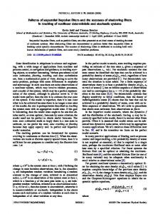
(15) in which case the output scale λ serves as the amplitude, and the input scale σ serves as the period. ω is a roughness parameter that serves a similar role to the input scale σ in (13). We now demonstrate how to construct appropriate covariance functions for a number of types of changepoint. Some examples of these are illustrated in Figure 1.
if p( φe | I ) is the uniform (4), and (P
∆e
φd,e ∆e Ke (φd,e , φi,e ) 1 d=1 ∆e Ke (φd,e , φi,e )
¯ e,f (φi,e ) = K
d=1 P∆ e
(e ∈ f ) , (e ∈ / f)
if p( φe | I ) is the discrete uniform (6). We now make the corresponding definition O �T �−1 ¯ e,f φ ¯T K Ke φu,e , φu,e m , u,e f ,
4.1
e
A drastic change in covariance
Suppose a function of interest is well-behaved except for a drastic change at the point xc , which separates the function into two regions with associated covariance functions K1 (·, ·; θ1 ) before xc and K2 (·, ·; θ2 ) after, where θ1 and θ2 represent the values of any hyperparameters associated with K1 and K2 , respectively. If
giving the posterior mean as � m � ¯T f rs m φ˚f z d , I ≃ T . ¯ ∅ rs m
Covariance functions for prediction in the presence of changepoints
(12)
T ¯T Note that m ∅ = m∅ (∅).
5
s04
v05 s02
s02
v05
v06
v04
s04
v07
s10
s06 s07
v05
v04
v07
s10
s06 s07
v06 s02
v06
s04
v07
s10
s06 s07
v05
v04
v04
v03
v03
v03
v03
v02
v02
v02
v02
v01s09 x01
x02
x03 x04 s01
x05
x06
v01s09 x01
s03 v04
v03 s01
v03 s01
v02
v02
x02 s02
x03 x04 s01
x05
v01s09 x01
x06
s03
v04
v01 x01
x02
x03
v01 x01
x02 s02
x02
x03 x04 s01
x05
s10
v06 s02
s04 v07
x06
s06 s07
v01s09 x01
x02
s03 v03
s01 v02
s01 v02
v01 x01
x02 s02
x05
x06
s03
v03
x03
x03 x04 s01
x03
v01 x01
x02 s02
x03
Figure 1: Example covariance functions for the modelling of data with changepoints, and associated example data that they might be appropriate for.
the change is so drastic that the observations before xc are completely uninformative about the observations after the changepoint; that is, if � � p y ≥xc z, I = p y ≥xc z ≥xc , I ,
I
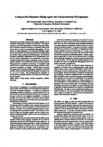
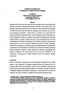
˚ y xc
Figure 2: Bayesian Network for the smooth drastic change model. I is the context, correlated with all other nodes.
where the subscripts indicate ranges of data segmented by xc (e.g. z ≥xc is the subset of z containing only observations after the changepoint), then the appropriate covariance function is trivial. This function can be modelled using the covariance function KA defined by K1 (x1 , x2 ; θ1 ) (x1 , x2 < xc ) KA (x1 , x2 ; θA ) , K2 (x1 , x2 ; θ2 ) (x1 , x2 ≥ xc ) . 0 (otherwise.) (16) The new set of hyperparameters θA , {θ1 , θ2 , xc } contains knowledge about the original hyperparameters of the covariance functions as well as the location of the changepoint. This covariance function is easily seen to be semi-positive definite and hence admissible.
covariance functions, their corresponding Gram matrices are positive semidefinite, and therefore eigenvalues of KA (x, x) are nonnegative.
4.2
A smooth drastic change in covariance
Suppose a continuous function of interest is best modelled by different covariance functions, before and after a changepoint xc . The function values after the changepoint are conditionally independent of the function values before, given the value at the changepoint itself. The Bayesian network for this probabilistic structure is depicted in Figure 2. This represents an extension to the drastic covariance described above; our two regions can be drastically different, but we can still enforce smoothness across the boundary between them. The changepoint separates the function into two regions with associated covariance functions K1 (·, ·; θ1 ) before xc and K2 (·, ·; θ2 ) after, where θ1 and θ2 represent the values of any hyperparameters associated with K1 and K2 , respectively. We introduce a further hyperparameter, kc , which represents the covariance
Theorem 1. KA is a valid covariance function. Proof. We show that any Gram matrix given by KA is positive semidefinite. Consider an arbitrary set of input points x in the domain of interest. By appropriately ordering the points in x, we may write the Gram matrix KA (x, x) as the block-diagonal matrix � � 0 K1 (x