Session USING SPREADSHEETS AND SIMULATION TO ENHANCE THE TEACHING OF PROBABILITY AND STATISTICS TO ENGINEERING STUDENTS Lorí Viali 1 Abstract The majority of engineering programs offer only one course in Statistics (usually 4 credits, sometimes 6) in their curriculum despite the importance it represents for the understanding of technical, scientific and even everyday questions. Besides this reduced number of available hours the content is extensive and generally includes Basic Statistics and the Probability Elements. The consequence is an unsatisfactory teaching and learning. In order to adjust the content to the number of available hours it is necessary to skip many topics that are usually seen only superficially. That is, when the schedule is on time, which is not usually the case. To improve this situation, this article presents experiences being conducted with the monitored use of computers and the support of a spreadsheet, as well as data simulation through the probabilistic models. The use of these resources increases the speed of comprehension, improves the understanding of a great deal of the content, and gets rid off the manual labor. Further, quality is obtained substituting much of the traditional oral exposure for an interactive teaching, where the student can experiment and manipulate large groups of data directly on the computer. A collateral effect of this approach is a greater familiarity with the computer and the spreadsheet, which are necessary resources for today's engineer.
the material being taught, the short number of examples, and many times, the lack of preparation and qualification of the teacher much of what the teacher intends to get through to his students is not taken advantage of. The student does not have access to a sufficient number of exercises. Further, he cannot make experiments on his own to see how 'everything really works'. Thus, the teaching of these courses is impaired by the absence of prerequisites for the understanding of the new knowledge being taught. Taking this into consideration, this paper proposes the use of simulation and computer experimentation as a way to involve the student more in what is being taught as well as increase the interactivity of teaching so that the student can really get down to business.
WHERE ARE THE M AIN D IFFICULTIES ? The main difficulty for those that teach courses that require a good understanding of mathematics is the heterogeneousness of the students in each class. Even though the level of knowledge of the students is below that desired, it is always possible to find a number of students who have their abilities more consistent with the knowledge required to deal with symbols and mathematical resources. Much the same way, in almost every class there are a number of students who present basic difficulties such as not being able to solve simple arithmetic computations. Another difficulty being faced is the low capacity for abstraction that the majority of the students present. This is a consequence of a learning process based on symbolic manipulation, lacking context and teachings that are not associated to concepts and definitions to support them, that is, teaching processes commonly know as memorization. The student memorizes enough to take the test and get a passing score but he is not able to understand the mathematical knowledge because this knowledge has not been presented in a structured manner. The contents are presented punctually but they are not related, making it easier for the student to forget the information as soon as it is no longer being used.
Index Terms New ways of teaching probability and statistics, Teaching using simulation, Teaching with spreadsheets.
INTRODUCTION The teaching of courses that involve abstract reasoning such as the ones in the area of Mathematics (probability, calculus, linear algebra, etc.) as well as those that involve and require modeling, that is, application of theoretical models, such as the area of Applied Mathematics (represented by Statistics), is done almost exclusively through lectures even though there is a fast growth of technology, especially in computers. The effort is made entirely by the teacher with very little participation from the student. Marcoulides [3] states: "The students are essentially passive participants in the pedagogical process with their activities restricted to listening, taking notes and reviewing the completed exercises." This creates lack of interest and low productivity. Due to the inability to arouse the student's interest, the quantity of information being more than the student can assimilate, the short time to think about 1
THE CONSEQUENCES It is possible to teach as usual and develop these courses in a very traditional manner, emphasizing isolated cases, solving punctual exercises and assessing with less criteria and more flexibility. That is, it is easy and tempting enough
Lorí Viali, PUCRS, DeStat - Famat, Av. Ipiranga, 6681, 90619-900 Porto Alegre, RS - Brasil
[email protected] UFRGS, DeStat - IM, Av. Bento Gonçalves, 9500, 91509-900 Porto Alegre, RS - Brasil
[email protected]
International Conference on Engineering Education
August 18–21, 2002, Manchester, U.K. 1
Session to follow the path of mediocrity, where the professor pretends he teaches and the student pretends he learns. However, this often results in the frustration of both the teacher and the student. Teaching well and consequently learning well involves a commitment from the teacher and the student. Taking into consideration that the students as well as the teachers are well intentioned, that is, one with the will to learn and the other with enthusiasm and ability to teach, there will still be a problem with a difficult solution. The difficulty lies in the student's past. The lack of prerequisites is a problem that cannot be solved immediately. It is practically impossible to solve a problem that is a result of the student's whole educational process. So how can we make teaching more productive and pleasant for all those involved? It is clear that the answer is not to be given now and I believe that it may never be given. However, it is necessary to keep on trying and, mainly to be careful not to repeat the failed method of teaching that has been proven not to work, in which the only ability developed is that of “manual labour.”
installed base and its relatively low price. Then, it is possible to program it to perform tasks not previously foreseen. What's more, the paradigm of the spreadsheet is known by the majority of the students, thus reducing the time spent teaching the use of a new software tool. The examples here presented refer to the Excel spreadsheet. Fortunately or unfortunately, it is the leader of this kind of software. This spreadsheet was released in 1987 in a version originally developed for Macintosh computers. The first version for Windows was labeled as 'two' to correspond to the original platform's version. In 1990 the third version was released, which included tools, ability to draw, support for additional programs and three-dimensional graphics. The forth version, the first to be really popular, was released in 1992. In 1993 the fifth version was released with impressive improvements such as multiple spreadsheets and support for the Visual Basic language. In 1995 the seventh version was released, commonly known as Excel 95 and the first one to be in 32 bites. The sixth version does not exist since Microsoft decided to rename its products for office in a way that all of them would have the same version. The eighth version was released in 1997, and it is known as Excel 97, which includes a new interface for the development of applications in Visual Basic. The ninth version was named Excel 2000. There are many alternatives to Excel. The problem is that the majority of them are practically unknown, with the exception of Lotus 1-2-3, which has already been very popular, and the exception of Quattro Pro. The other alternatives can be found with a very careful search of the Internet. Further, there is practically no literature on Statistics teaching with these spreadsheets.
THE PROPOSAL The proposal is to provide a teaching that eliminates or reduces most of the work of the student. Further, a teaching that excludes the task of filling blackboards with exercises for the student to spend most of his time simply copying. From the notes of the teacher to the board and from the board to the student's notebooks without going through the head of either one. Knowledge has to be proposed, discussed, assessed, analyzed, and as often as possible, reproduced as if it were being newly discovered. The teacher should use his experience to point out the most obscure points, the difficulties to be encountered and to propose tasks and exercises that will improve the comprehension of the concepts and definitions. Further, he should also show relations and interrelations between various segments, in a way that the content is understood as a structured group and not just a collection of recipes. Statistics is an applied course and thus it involves theoretical models as well as practical knowledge. Emphasizing the similarities and differences between theory and practice is essential. It is common to find a mix of probability and statistics in didactic texts, which often confuses the student. The most appropriate thing to do is to emphasize the differences so that the similarities will then be more apparent.
SIMULATION Statistics works with the description, summary and interpretation of data. Collecting data is not an easy task and it is a time consuming job. In an efficient system of teaching, the data should be readily available and this can only be done through a simulation of these data. Most of the statistical procedures involve some supposition about the correspondent theoretical model. In order to build valid confidence intervals it is necessary to suppose that the sampled population has a normal distribution. How do you obtain data that fit this model? One option would be to conduct a real experiment or collect data that knowingly have this behavior. However, usually this is not an option due to a series of time limitations and availability of such sources of variation. Traditionally simulation would be used as a last resource, at least theoretically. On the other hand, what has been observed is that simulation is largely employed in all areas of knowledge as one of the main techniques of discrete systems analysis, as a verifier of analytical solutions, and fundamentally as a data provider in the experiments, problem solving, demonstration of properties and even in
THE SPREADSHEETS The spreadsheets, especially Excel, are becoming instructional resources in Statistics' laboratories. Besides the typical resources they also offer a great number of statistical and probabilistic functions, even though they are quite limited. The main advantage of a spreadsheet is its huge International Conference on Engineering Education
August 18–21, 2002, Manchester, U.K. 2
Session proving theorems. In such case the technique used is Monte Carlo, that is, the production of random values and distributions. The use of computational packages freed teachers and students of Statistics and Probability courses from the boredom caused by excessive work in doing a great number of irrelevant calculations that do not add anything in terms of learning. However, conventional software such as Minitab, SAS, SPSS, Statgraphics, Statistica and Systat haven't been helping much in the understanding of sub adjacent concepts. The students do not ponder upon what they are doing and why they are doing it. They simply throw data around and apply the test, according to Sterling. According to Merrill [4], simulation is a valuable tutorial tool for the following reasons: a.) It involves fewer risks than reality. If a student does something wrong during a simulation he simply restarts. In real systems mistakes would be fatal but in a simulation they can only cause frustration. The mistake will become experience and it will be repeated less often in the future. b.) The training costs are reduced. A piloting error in a real airplane would cost a large sum of money without mentioning the lives lost. c.) It is usually more convenient than real training since it allows training more than one student at a time. When you work in a computer in a laboratory you won't be subjected to time restrictions, whether it is day or night, or if the real equipment is broken or in maintenance. d.) Simulation minimizes the effects of time. Some phenomena take a long time to happen and in a computer simulation this can be reduced in a way that the phenomena can be observed many times in a much shorter period of time. e.) Experiences in simulation can be repeated. The students can repeat an experience as many times as necessary to understand them and face them with ability. Many learning difficulties occur due to having only one statistical vision of the natural and artificial systems' representations. This is the only way possible with a book. On the other hand in a computer the models can be more dynamic.
The RAND() function has no arguments and returns an uniform distribution in the interval [0;1]. These numbers are denominated pseudorandom. This function is denominated by Excel as volatile, that is, it is recalculated every time that a spreadsheet cell is calculated. To prevent this from happening one can transform the formula into a random number. In order to do this, it is necessary to select the cell that contains the formula, click on the formula bar and type F9. After this procedure, a number that will not alter will appear when you click on a specific cell of interest. This is the most important function because it can be used as a foundation to create values for any other probability distribution, for instance, simulating the distribution of the distance gone through a car traveling in a highway from the city A to city B.. Taking into account that the path has exactly 90 km, one can simulate the variable "distance gone through" from the city A til city B through: RAND()*(b-a) + a, where a = 0 and b = 90. Thus, the simulation of the variable would be 90* RAND(). In order to simulate the behavior of an exponential distribution of parameter λ, one should start with the distribution function F(x) =1- eλx and make this expression equal to a variable U or RAND(). This can be done in the following manner u = 1- eλx ; eλx = 1 - u; λx = ln(1 - u); x = ln(1 - u)/ λ. But the expected value of the exponential is equal to the parameter inverse, that is, µ = E(X) = 1/ λ, then the expression above turns into: X = ln(1 -U)/ λ = µ.ln(1 - U).
RESOURCES FOR S IMULATION IN EXCEL
In this way if it were necessary to simulate the variable "time elapsed between two cars", where the mean was 30 seconds, the expression to simulate this experiment would be: X = 30.ln(1 - U). Considering the spreadsheet functions it would be necessary to type in a spreadsheet cell the following: = 30*LN(1 - RAND()), an expression that will create values of an exponential distribution with a mean of 30 and parameter 1/30. On contrary to the previous function, the RANDBETWEEN(bottom; top) function requires two parameters. This function can be seen as an specialization of
FIGURE 1 THE RESOURCE GENERATION OF RANDOM NUMBER"
The Monte Carlo simulation resources of Excel can be divided into two categories. Those that are activated through the fx icon in the Paste function and those that are part of the "Analysis Toolpack" library. This library can be activated through the "Tools" menu, sub-menu "Data Analysis….” In the first category mentioned there are two functions that play important roles to simulate distributions, which Excel does not present in the data analysis resource. These functions are RAND() and RANDBETWEEN (bottom; top).
International Conference on Engineering Education
August 18–21, 2002, Manchester, U.K. 3
Session the RAND() function. However, on contrary to the RAND() function, it only creates whole values and thus it can be used to simulate just discrete variables. Within the available "Analysis Tools" there is an item called "Random Number Generation", "Figure 1", which must be activated in order to simulate the values of some discrete and continuous models usually seen in the contents taught in Probability and Statistic courses. "Figure 2" shows a dialogue box of the item, "Random Number Generation".
Weibull and Gama distributions, which are frequently used models in engineering applications.
USING S IMULATION IN TEACHING The values simulated through the previously mentioned functions can be used in many ways in order to illustrate and facilitate the understanding of statistical concepts. The first example to be given is in the area of Descriptive Statistics, where one can simulate a large quantity of values in a discrete distribution in order to illustrate how to group data in frequency distributions by point or values. In this case, both the RANDBETWEEN (bottom; top) function, which creates integer values between two specific values, as well as the "Binomial", "Poisson" and "Discrete" functions (included in the "Data Analysis…" function) can be used. These functions can simulate a great number of applications and variables that describe phenomena or experiments. The following examples can be simulated: the traditional experiments with dice and decks of cards through the RANDETWEEN (bottom; top) function; the possible answers of a group of people about their political preferences or the number of damaged objects in a allotment of a production line using the Binomial model; the number of problems found in energy supply; the number of phone calls in a central telephone station and a vast number of systems that deal with lines through the Poisson model. Those experiences that do not fit into a known model can be simulated through the empirical distribution with the use of the "Discrete" option.
FIGURE 2 THE TEXT BOX "GENERATION OF RANDON NUMBER"
The third line on figure 2, denominated "Distribution", shows a cascade menu that provides seven options for distributions that can be simulated. Of these seven options, three are discrete variables: "Bernoulli", "Binomial" and "Poisson.” There is a forth option, denominated "Discrete", that allows the simulation of an empirical distribution provided by the user. The absence of a hypergeometric distribution should be mentioned. It is very unfortunate since the algorithm used for the creation of such distribution is not elementary and this model is used very often in the sampling theory. Of the three options left, two are continuous random variables, "Uniform" and "Normal". The last option, called "Patterned", does not create random values but it creates sequences with a defined behavior. It is a mistake to include it among the other distributions since the results of this one are completely foreseeable. There are also some important omissions to be mentioned among the continuous variables. The exponential distribution, fundamental in any textbook of elementary probability is missing. Also lacking is the possibility for the user to generate an empirical continuous distribution, contrary to the discrete case. Without mentioning the omission of the
FIGURE 3 AN EXAMPLE OF SIMULATION ON DESCRIPTIVE STATISTICS
"Figure 3" presents the creation of 500 values of the variable X = "number of cars per minute that drive through a specific crossing in the city”, through Poisson distribuition.
International Conference on Engineering Education
August 18–21, 2002, Manchester, U.K. 4
Session The values created are on column A of the spreadsheet and the summary of the values through the distribution of frequency by points or values is found on columns C and D. An experiment that could take some hours or even days to be concluded can be simulated in just a few seconds.
illustrate the behavior of the sampling error varying inversely the square root of the sampling size. "Figure 5" illustrates this experiment using only one simulated element, that is, the population that has the exponential form. This experiment was simulated using an exponential mean of 30, through the expression =30* LN(1 RANDOM()), once the spreadsheet does not have resources for exponential simulation. Further, some statistics from the population are shown such as the minimum and maximum values created, as well as the mean and standard deviation. The theoretical values of the mean and standard deviation of the population are presented next to it, as well as the expectancy for the means of the samples and the sample standard deviation (standard error or sampling error). "Figure 6" shows the diagram of the means of the samples of size n = 9, which were taken from the population presented on figure 5. The statistics of minimum and maximum value, the mean (sampling expectancy) and standard deviation of the mean are also shown the same way. The minimum value presented in figure 5, as 0,06 is now 8,25. The maximum value presented in figure four, as 183,12 is now 74,35. This way the student can see in a practical and interactive manner how things happen. He can manipulate the size of the sample directly on the spreadsheet and witness the decrease that occurs in the variability of the sampling means. He can also witness its consequence in the decrease of the sampling error, which at first was 30 and now is 10,49. This number is very close to the theoretical value, which would be:
FIGURE 4 CLASSIC VERSUS FREQUENTIAL CONCEPTS OF PROBABILITY
A second example is the illustration of the frequency concept of probability. It is a concept that can cause many doubts because it involves the passing of time and thus it does not allow visualization. Furthermore, it is not completely intuitive. The RAND() function is used together with the logical IF(logical_test; value_if_true; value_if_false) function in the following manner: IF(RAND() > 0,5; "Head; "Tail"). Head = 1 and Tail = 0 can be used in order to make the computation easier. To simulate the frequency concept of probability, the throwing of a coin can be simulated, for example, 500 times and calculate the relative frequencies and then compare the result with the probability obtained by the classical concept, which is 50%. Using a graphic of these results it is easy to notice that as the number of experiences increases the relative frequency (empirical probability) tends to vary less and less, approximating the classical value of 50%. "Figure four" illustrates this experiment. The creation of values and random distributions is also very useful in the sampling theory. Students frequently misunderstand the concept of sampling distributions and especially the concept of sampling error. On the other hand, it is fundamental to the understanding of the estimation theory and hypothesis testing. A simulation experiment, showing how samples taken from various populations lead invariable to a normal distribution, illustrates the central limit theorem and at the same time, it can illustrate the behavior of the mean random variable. The example can
FIGURE 5 SIMULATED EXPONENTIAL POPULATION
σX =
σ
=
σ
=
30 = 10 3
n 9 It is important to notice the form of the graph of figure 6, which shows that even with a small sample of n = 9
International Conference on Engineering Education
August 18–21, 2002, Manchester, U.K. 5
Session REFERENCES
(theoretically the sample size should be n = 30) one can have a graph form that resemble the normal curve. This is a valuable vision to the student because he can witness on his own something that otherwise he only see in some formulas quickly enunciated in a classroom. Here he can visualize and even manipulate in order to notice that the traditional form would only be one more formula or one more concept to be memorized.
[1] Bisgaard, S∅ ren. "Teaching Statistics to Engineers", The American Statistician, vol. 45, n. 4, Nov. 1991, p. 274-283. [2] Chang, Ted C.; Lohr, Sharon L., C. Mclaren, Graham. "Teaching Survey Sampling Using Simulation", The American Statistician, v. 46, n. 3, Aug. 1992, p. 232237. [3]
Marcoulides, George A. "Improving Learner Performance with Computer Based Programs". Journal of Educational Computing Research, v. 6, n. 2, 1990, p. 147-155. [4] Merril, Paul F et al. "Computers in Education.” Needhan Heights, Massachusetts: Simon & Schuster, 1996, 386 p. [5] Nascimento, João Agnaldo do. "O Ensino e Programa de Estatística para a Graduação de Engenharia.” ABENGE: Revista de Ensino de Engenharia. n 20, segundo semestre de 1998, p. 3-9. [6] Power, Daniel. "A Brief History of Spreadsheets" [online] http://dss.cba.uni.edu/dss/sshistory.html. [7] Smith, P. R.; Pollard, D. "The Role of Computer Simulations in Engineering Education", Computers in Education, v. 10, n. 3, 1986, p. 335-40. FIGURE 6
[8] Sterling, Joan; Gray, Mary W., "The Effect of Simulation Software on Students’ Attitudes and Understanding in Introductory Statistics.” Journal of Computers in Mathematics and Science Teaching, v. 10, n. 4, Summer 1991, p. 51-56. [9] Viali, Lorí. "Simulação de Sistemas de Manufatura.” Dissertação de Mestrado em Engenharia de Produção, Florianópolis: UFSC (Universidade Federal de Santa Catarina), Out. 1991, 186 p.
SAMPLES OF SIZE N = 9 FROM AN EXPONENTIAL POPULATION
CONCLUSION It is impossible to deny the fact that computers have changed everyday life and increased the speed of access to knowledge. However, despite the apparent use of computers in all activities, its use in education is still very limited. Traditional education still fights the use of computers in the area of the exact sciences and the black board and chalk are still the main resources used by the teachers. In this article we attempted to show some of the simulation resources with the use of Excel's spreadsheet to improve the understanding of the contents of probability and statistics. Of course, these resources do no need to remain limited to this course; many other courses can take advantage of computational resources and, in particular, the spreadsheet. It is true that there are very sophisticated computational resources for educational support in the area of mathematics and statistics. However, the main problem rests in the fact that these resources involve a very slow learning curve, a luxury that the majority of the students with a great deal of hours dedicated to their classes cannot give themselves. Thus, the spreadsheet is an accessible and easy to use resource, without mentioning the fact that a great part of the students already know how to use it. Even considering its limitations, the spreadsheet is the resource that offers the best cost-benefit in terms of didactic resources.
International Conference on Engineering Education
August 18–21, 2002, Manchester, U.K. 6