Energy and Power Engineering, 2013, 5, 161-170 http://dx.doi.org/10.4236/epe.2013.52016 Published Online March 2013 (http://www.scirp.org/journal/epe)
Short-Term Scheduling of Combined Cycle Units Using Mixed Integer Linear Programming Solution Juan Alemany1, Diego Moitre1, Herminio Pinto2, Fernando Magnago1,2
1
Department of Electrical & Electronic Engineering, National University of Rio Cuarto, Rio Cuarto, Argentina 2 Nexant Inc., Chandler, USA Email:
[email protected] Received January 12, 2013; revised February 15, 2013; accepted February 28, 2013
ABSTRACT Combined cycle plants (CCs) are broadly used all over the world. The inclusion of CCs into the optimal resource scheduling causes difficulties because they can be operated in different operating configuration modes based on the number of combustion and steam turbines. In this paper a model CCs based on a mixed integer linear programming approach to be included into an optimal short term resource optimization problem is presented. The proposed method allows modeling of CCs in different modes of operation taking into account the non convex operating costs for the different combined cycle mode of operation. Keywords: Combined Cycle Plants; Unit Commitment; Mixed Integer Linear Programming
1. Introduction The gas-turbine combined cycle plant has been used extensively in power generation, representing the great majority of new generating unit installations across the globe. Combined cycle (CC) technology is now well established, becoming one of the most effective energy conversion technology at present [1,2]. The progress on CC generation technology allowed improving their thermal efficiency up to 50% approximatelly. In addition, CCs present other advantages such as better environmental performance, reducing greenhouse gases, short construction lead time and low capital cost to power ratio. Moreover, the price of natural gas, which is the primary fuel used for combined cycle plants, dropped. As an example of CCs use evolution, Figure 1 shows the generation growth in Argentina since 1992 [3]. From the figure it can be seen the significant increase on the use of combined cycle plants. Despite of their benefits, the utilization of CCs created new challenges. One of these challenges is the inclusion of combined cycle plants into the unit commitment problem (UC). Modeling of CCs for UC studies is quite difficult due to the tight iteraction between the gas turbine and the steam turbine generating units. These units have different operating modes; each of the operating modes has parameters such as limits or incremental heat rate that can differ considerably from each other depending on which mode is operating at the time. Therefore, the Copyright © 2013 SciRes.
problem needs to be expanded to determine which operating mode the combined cycle units have to be in operation at each time. Several researches have been conducted to include detailed CC model into the UC related problems. A flexible modeling approach in order to take the multiple possible configurations into account is described in [4]. The model is based on a single unit dynamic approach that can be incorporated into a Lagrange Relaxation unit commitment algorithm. Reference [5] considers the inclusion of combined cycle plants into an optimal short-term resource optimization. The short-term resource scheduling is realized through an Augmented Lagrange Relaxation technique. The optimal commitment of combined cycle plants is obtained by applying a dynamic programming algorithm for a previously defined combined cycle plant state space. In [6] a method for establishing the state space diagram of combined cycle units for applying dynamic programming and Lagrange Relaxation to the security constrained short-term scheduling problem is presented. Several studies verify the advantages of combined cycle units in competitive electricity markets. Combined cycle models were also included into economic dispatch problems based on Genetic Algorithms, Evolutionary Programming, and Particle Swarm techniques [7]. The CC incremental heat cost curve is approximated by a 4th polynomial in order to consider the effect of different operating modes. The non-convex nature of the CCs incremental cost curve is highlighted. EPE
162
J. ALEMANY
ST
CT
ET AL.
DI
CC
HY
NU
35
Installed Capacity (GW)
30 25 20 15 10 5
2011
2010
2009
2008
2007
2006
2005
2004
2003
2002
2001
2000
1999
1998
1997
1996
1995
1994
1993
1992
0
Year
Figure 1. Evolution of electricity generation in Argentina.
Recently, advances on mixed integer programing techniques (MIP) allow applying this technique to very largescale, time-varying, non-convex, mixed-integer modeling and optimization, such as unit commitment problems. A mixed integer programing approach that allows a rigorous modeling to obtain the optimal response of thermal unit to an electricity spot market is proposed in [8]. An extension of this work is presented in [9] where a MIP formulation for the unit commitment problem of thermal units that allows modeling of non-convex operating costs and exponential start up costs is developed. Furthermore, a MIP solution for solving the PJM unit commitment problem is described in [10]. The paper explains many of the inherent problems associated with MIP solutions and illustrates how these issues were dealt with to provide a fast, accurate, and robust MIP solution. The first formulation of a combined cycle unit model using MIP is presented in [11] where a detailed formulation of a price-based unit commitment (PBUC) problem based on the MIP method is developed. The PBUC solution by utilizing MIP is compared with that of Lagrange Relaxation method. As another alternative, a simplified combined-cycled unit model to solve the related mixed integer linear programming-based UC problem is shown in [12]. Although the model is simple, presents the disadvantage of loosing solution accuracy. Another alternative approach that model combustion turbines and steam turbines individually is presented in [13]. They applied the MIP method to solve the UC problem, where the output dispatch for CC plants is set for Copyright © 2013 SciRes.
individual gas turbine and steam turbine generating units. According to what has been said above, it is evident that CC has acquired great relevance, particularly the development of models used for UC problems. The aim of this paper is to develop a general and accurate CC model purposely designed with the idea that it could be easily included into any optimal short-term resource optimization problem based on a mixed integer linear programing approach. The proposed model, which has taken into account studies previously done by different researchers, includes non-convex cost curves and exponential start up cost curves for each operational CC mode, keeping the number of constraints to the minimum. The paper is organized as follows; first the combined cycle model based on different modes of operation is presented, then the unit commitment problem formulation based on mixed integer linear programming approach including CC units is described. After that, a numerical example is given, finally presents the most important conclusions of the paper.
2. Combined Cycle Units Typically, a combined cycle unit comprises of several combustion turbines (CT) and several steam turbines (ST), the waste heat from the CTs is used to produce the steam to generate additional power using STs, and this process enhances the efficiency of electricity generation. Depending on the number of CTs and STs, combined cycle units can operate in different configurations, also EPE
J. ALEMANY
known as modes. Each configuration is determined based on a possible combination of CTs and STs, having a determined generating region and an incremental heat rate curve. Configurations or modes with STs are more efficients; however, since the modes are restricted due to the generation region may not be more efficient for a particular load and a particular simulation period. As an illustration, considering a combined cycle unit with two CTs and one STs, the related possible configurations are shown in Table 1, the state space is shown in Figure 2. This four mode example is used to illustrate the problem without losing generality and can be extended for any CT + ST configuration. Figure 3 and Table 2 show typical incremental heat rate curves and generation regions for this particular combined cycle unit. Some of the incremental heat rate curves are not monotonically increasing with generation or are monotonically increasing but not convex. Therefore, if this particular condition is not considered during the optimization, the algorithm may fail to find the minimum solution. In addition, combined cycle units have other constraints such as transition between modes and minimum time on and off for each of the modes. Furthermore, there are modes that, for a particular period, can not be eligible, for example, a CT may need to be in service for several hours prior to turn on an associated ST. Considering all these issues, a mixed integer formulation for combined cycle plants compatible with general MIP software is described next.
163
ET AL.
3. MIP Algoritm 3.1. List of Symbols t: Index for simulation hours. b: Index for cost curve segments. n: Index for startup cost curve. cc: Index for combined cycle units. m: Index for combined cycle modes. T: Total number of simulation hours. G: Total number of thermal units. B: Total number of segments for production cost curve. N: Total number of startup cost curve steps. CC: Total number of combined cycle units. M: Total number of combined cycle modes. Cpg,t: Production cost for unit g at hour t [$/h]. Cpm,t: Production cost for mode m at hour t [$/h]. Cupg,t: Startup cost for unit g at hour t [$]. Cupm,t: Startup cost for mode m at hour t [$]. pg,t: Active generation for unit g at hour t [MW]. pm,t: Active generation for mode m at hour t [MW]. Table 1. Combined cycle mode example. Mode
Configuration
0
CC out of service (mode off)
1
CT
2
CT + CT
3
CT + ST
4
CT + CT + ST
Figure 2. State space transition diagram.
Copyright © 2013 SciRes.
EPE
164
J. ALEMANY
ET AL.
STHm: Maximum number of hours that mode m can be off [h]. MUm: Minimum up time for mode m [h]. MDm: Minimum down time for mode m [h]. Tmoff : Number of hours mode m has been off at t = 0 [h]. Tmon : Number of hours mode m has been on at t = 0 [h].
3.2. Problem Formulation
Figure 3. Combined cycle modes incremental heat rate curves. Table 2. CCs modes incremental heat rate. Mode 1
Mode 2
Mode 3
T
$/h
MW
$/h
MW
$/h
MW
$/h
20
818
40
1636
30
818
50
1636
30
1044
60
2088
50
1044
70
2088
40
1272
80
2544
70
1272
90
2544
50
1501
100
3002
90
1501
110
3002
60
1731
120
3462
100
1731
130
3462
70
1963
140
3926
120
1963
180
3926
80
2196
160
4393
135
2196
215
4393
rg,t: Active reserve contribution of unit g, hour t [MW]. rm,t: Active reserve contribution of mode m, hour t [MW]. δb,m,t: Active generation for segment b, mode m, hour t [MW]. hmoff,t : Counter of hours off for mode m, hour t. dvm,t: Slack variable for the discretization of the startup cost function of mode m, hour t. ug,t: Binary state variable for unit g, hour t. um,t: Binary state variable for mode m, hour t. sm,t: Startup variable for mode m, hour t. zm,t: Shutdown variable for mode m, hour t. jb,m,t: Activation variable for segment b, mode m, hour t. wn,m,t: Binary variable which activates the step n of the stepwise startup cost of mode m at hour t. ym,t: Startup variable for transitions to mode m, hour t. Dt: System demand at time t [MW]. Rt: System spinning reserve requirement at time t [MW]. cm: Fixed cost for mode m [$/h]. Fb,m: Slope for segment b, mode m [$/MWh]. Pm : Maximum capacity for mode m [MW]. Pm: Minimum capacity for mode m [MW]. Pb,m: Upper limit for segment b, mode m [MW]. Kn,m: Cost for startup cost step n, mode m [$/h].
G
min Cpg ,t Cupg ,t
Mode 4
MW
Copyright © 2013 SciRes.
The unit commitment problem (UC) can be formulated as a minimization problem which main objective is to determine the generation dispatch to supply the demand and reserve requirements at minimum cost over a period of time. Mathematically can be represented as follow: u, p
t 1 g 1
Subject to: G
Dt U g ,t pg ,t 0 g 1
(1)
G
Rt Dt rg ,t 0 g 1
Combined cycle plants can be included into the general UC formulation by modifying the cost function and adding new constraints. The changes needed for the two components of the objective function represented by Equation (1), are described below.
3.3. Production Cost Considering the incremental cost function represented by the piecewise function of Figure 4, the production cost function for each mode m at a simulation period t, can be formulated as: B
Cpm ,t cm um,t Fb , m b , m,t
(2)
b 1
Subject to: B
pm,t Pm um ,t b , m,t
(3)
b 1
For all the segments inside the curve the constraints are:
P
b,m
Pb 1, m jb , m,t b , m,t
b , m,t Pb, m Pb 1, m jb 1, m,t
(4)
For each mode, MW capacity restrictions apply:
Pm um,t pm,t
(5)
Pm um,t pm,t
(6)
EPE
J. ALEMANY
165
ET AL.
Figure 4. Piece wise incremental cost curve per mode.
Finally, the following restrictions related to the MW per segment, and the binary conditions of the index respectively are:
b, m,t 0, jb, m ,t 0,1
(7)
3.4. Startup Costs For the startup cost model, the transition cost not only from the off state but between modes needs to be considered. Figure 5 shows a typical exponential start up cost function and the discrete representation. that takes into account the First, the counter hoff m ,t hours that the mode m has been off is represented and formulated as follow:
segment activation w(n,m,t) are: N 1
dvm,t nwn , m,t hmoff,t 1
(15)
n 1
dvm ,t STH m wN , m ,t ym ,t 1 , dvm,t NwN , m,t (16)
These constraints are related to the logical variables as follow: ymt ,t
mf FR
ymt ,t
zmf ,t
mtTO
smt ,t
(17)
zmf ,t smt ,t
(18)
um,t umt ,t 1 sm,t zm,t
(19)
mf FR
hmoff,t hmoff,t 1 1
(8)
sm,t zm ,t 1
(20)
hmoff,t STH m 1 um,t hmoff,t 1 1
(9)
sm,t um ,t 0, um,t , sm ,t , zm,t , ym,t 0,1
(21)
hmoff,t STH m 1 um,t 0 hmoff,t 0 STH m Tmoff T
(10) (11) (12)
Then, based on the discretized approximation, a mathematical formulation for the start up cost is included per mode m and per simulation period t: N
Cupm,t K n , m wn , m
(13)
n 1
Subject to: N
wn,m,t ym,t , wn, m,t 0,1
(14)
n 1
The constraints that relate the slack variable dv(m,t) with the start up transition binary variable y(m,t) and the startup Copyright © 2013 SciRes.
Then, the formulation explained in Subsection 3.1, can be reformulated to include combined cycle plants: T G CC min Cpg ,t Cupg ,t Cpm,t Cupm, y (22) u, p t 1 g 1 cc 1
Subject to: G
CC M
g 1
cc 1 m 1
Dt u g ,t pg ,t um,t pm,t 0 G
CC M
g 1
cc 1 m 1
Rt Dt rg ,t rm,t 0
(23) (24)
And the restrictions developed in this subsection and 3.3. In addition to these constraints which are related to the production and start up cost, further constraints are needed. These constraints are related to the relationship between configuration status, and on/off conditions. EPE
166
J. ALEMANY
ET AL.
Figure 5. Exponential startup cost discretization.
3.5. Configuration Status
t
For all simulation periods t, only one CC mode can be selected: M
um , t 1
(25)
m 1
The restriction for the transition between mode “from” mf and mode “to” mt can be represented as follow: mf NFSmt
umf ,t 1 umt ,t
umf ,t 1
sm , l u m , t
(28)
zm , l 1 um , t
(29)
l t MU m 1 t
l t MDm 1
For the initial period, the number of periods the mode is on or off need to be considered:
3.6. Mode Transition
(26)
Tmoff
um ,l 0
(30)
l 0
Tmon
1 um ,l 0
(31)
l 0
(27)
umt ,t
Table 3 illustrates an example for the definition of set NFSm for the 2CT-1ST case. This set is defined based on the state space transition diagram of Figure 2.
Based on the general UC problem formulation, it was modified to include the combined cycle model into the MIP formulation, next section discusses the results considering a typical power system and the addition of combined cycle modeled as explained in this section.
3.7. Minimum On/Off Conditions
4. Numerical Results
The modes also have restrictions due to the minimum time on and minimum time off that the generator needs to remain before the transition to another mode, these restrictions can be formulated as:
Numerical results obtained by the proposed solution model are shown in this section. The MIP problem is solved using GAMS, and the optimization engine selected is CPLEX 12.0. Tables 4 and 5 illustrate the CPLEX option setup. The test system presented in [14] is used as the base system. This system has ten generation units which are all different in term of production and start up cost. The total generating capacity is 1662 MW with a system peak load of 1500 MW. Then, to carry out the simulations, two different systems are created. First the original system is modified to include a combined cycle plant. Coal fired units 6, 7, and 8 are chosen and its original charac-
mtNFS mf
Table 3. Transition mode variables. mt
NFSmt
mf
NFSmf
1
0, 1, 2, 3
1
0, 1, 2, 3
2
1, 2, 4
2
1, 2, 4
3
1, 3, 4
3
1, 3, 4
4
2, 3, 4
4
2, 3, 4
Copyright © 2013 SciRes.
EPE
J. ALEMANY
167
ET AL.
Table 4. CPLEX options. CPLEX option
Value
Description Force an optimal solution search
Relative tol.
0
Backtracking tol.
0
Best-bound search
MIP tactic emphasize
1
Feasibility over optimality
Objective upper bound
System dependant
Based on a dispatch with all units in service
Objective lower bound
System dependant
Based on a dispatch with an heuristic priority order without reserve requirements
startup costs
and minimum on/off times.
Priorities
1
Activate the use of priorities for branching
Branching rule
1
Branch on variables with maximum infeasibility
Table 5. Integer variable priorities. Level 1
um,t
Level 2 Level 3
Table 6. Commitment MW including a CC.
sm,t jb,m,t
wn,m,t
ym,t
zm,t dvm,t
hmoff,t
teristics are modified in order to model them as a combined cycle model. This allows to study the differences between a typical CC modeled as an equivalent thermal plant and modeled taking into consideration the different modes of operation. Table 6 shows the commitment results for one day simulation period, the 2CTs and 1ST are based on units 6, 7, and 8 respectively. The Table illustrates the dispatch for some of the simulation hours. Table 7 illustrates the cost differences of both cases, modelling the generator as an equivalent thermal plant or modeling the generator using the proposed combined cycle model. The simulations are performed for two different time horizons, in addition it shows the total simulation time for both models. Then, a 20 generating system is built by duplicating the original system following the same pattern, the results for this system are shown in Table 8. In addition, the calculations and comparisons are repeated for different load profiles, Table 9 shows the results for a 24 h simulation period for both systems, changing the base load by 10%, Figure 6 illustrates the load profile used during the simulations. Figure 7 shows the matrix structure of this formulation applied to the 10 generation unit system, from where it can be seen the sparse structure of the matrix. For this system, after the presolve stage, the MIP array size is 144 columns and 292 rows, having 2% of nonzero elements. The development approach gives optimal, mutually exclusive commitment of the combined cycle plant configurations. Results illustrate the impact of explicitly model of combined cycle units on minimizing the cost of supplying the load. The additional computer time required to schedule a combined cycle unit with multiple configurations depends on the number of configurations, the number of transitions, the minumum up times, the transition times and the load profile. Copyright © 2013 SciRes.
Hr
9
10
11
12
13
14
20
21
G.
MW
MW
MW
MW
MW
MW
MW
MW
Th1
455
455
455
455
455
455
455
455
Th2
455
455
455
455
455
455
455
455
Th3
130
130
130
130
130
130
130
130
Th4
130
130
130
130
130
130
130
130
Th5
90
162
162
162
162
90
162
90
Th6
20
38
78
80
38
20
20
20
Th7
0
0
0
0
0
0
0
0
Th8
0
0
10
10
0
0
10
0
Th9
0
0
10
10
0
0
0
0
Th10
0
0
0
0
0
0
0
0
Mod CC
MW
MW
MW
MW
MW
MW
MW
MW
1
20
0
20
0
0
20
38
20
2
0
0
0
0
0
0
0
0
3
0
30
0
68
30
0
0
0
4
0
0
0
0
0
0
0
0
5. Conclusion Nowadays, the use of combined cycle plants becomes popular due to their advantages. Therefore, it is very important to have an accurate model to include combined cycle plants into a unit commitment problem. This paper presents a combined cycle model for optimal resource optimization problems based on mixed integer linear programming approach. Based on previous general models developed for thermal plants in [8], the main focus of this paper was to develop a general CC model that can be easily included into a MILP based UC model. Test results evidence that explicit model of a combined cycle units can save operating costs. Furthermore, the paper illustrates how the proposed model can be included into a unit commitment MILP formulation, having as its main advantage the general modeling of mode incremental cost curves including non convex ones and facilitates the EPE
168
J. ALEMANY
ET AL.
Table 7. Cost comparison 10 Gen system. CC Model 24 h
Th Model 24 h
CC Model 74 h
Th Model 74 h 16,195
Model
Variables
5395
5395
16,195
Statistic
Equations
9306
9306
28,206
28,206
Discrete Vars
3594
3498
10,794
10,498
Non Zero Elements
34,313
34,313
104,613
104,613
MIP
Objective
561,411
564,527
1,680,808
1,688,410
Solution
Time
2.147
1.352
8.261
5.488
Th Model 74 h
Table 8. Cost comparison 20 Gen System. CC Model 24 h
Th Model 24 h
CC Model 74 h
Model
Variables
10,739
10,739
32,239
2239
Statistic
Equations
18,494
18,494
56,044
56,044
Discrete Vars
7188
6996
21,588
20,996
Non Zero Elements
68,633
68,633
209,233
209,233
MIP
Objective
1,097,756
1,100,278
3,240,969
3,253,183
Solution
Time
10.257
8.574
100.858
55.145
Table 9. Cost comparison, load variation. 10 Gen
Base
−10
+10
561,411
496,678
632,571
CC Model
Objective Time
2.147
2.183
1.961
Th Model
Objective
564,527
498,158
621,863
Time
1.352
1.896
1.803
Objective
1,097,756
855,676
1,231,515
Time
10.257
16.247
7.921
Objective
1,100,278
856,572
1,239,888
Time
8.574
12.376
2.645
20 Gen CC Model Th Model
Figure 6. Load profile for base case and 10% variation. Copyright © 2013 SciRes.
EPE
J. ALEMANY
ET AL.
169
Figure 7. MIP matrix structure.
incorporation of feasible and non convex constraints which are present in this type of studies and very difficult to solve.
REFERENCES [1]
[2]
H. Rudnick and J. Zolezzi, “Electric Sector Deregulation and Restructuring in Latin America: Lessons to Be Learn and Possible Waysforward,” IEEE Proceedings Generation, Transmission and Distribution, Vol. 148, No. 2, 2001, pp. 180-184. doi:10.1049/ip-gtd:20010230 E. Battisti, G. Casolino, F. Rossi and M. Russo, “Economical Considerations about Combined Cycle Power Plant Control in Deregulated Markets,” International Journal of Electrical Power and Energy Systems, Vol. 28, No. 4, 2006, pp. 284-192. doi:10.1016/j.ijepes.2005.12.003
pp. 189-194. [6]
B. Lu and M. Shahidehpour, “Short-Term Scheduling of Combined Cycle Units,” IEEE Transactions on Power Systems, Vol. 19, No. 3, 2000, pp. 1616-1625.
[7]
F. Gao and G. B. Sheble, “Stochastic Optimization Techniques for Economic Dispatch with Combined Cycle Units,” Proceedings of 9th International Conference on Probabilistic Methods Applied to Power System, Stockholm, June 2006, pp. 1022-1034.
[8]
J. Arroyo and A. Conejo, “Optimal Response of a Thermal Unit to an Electricity Spot Market,” IEEE Transactions on Power Systems, Vol. 15, No. 3, 2000, pp. 10981104. doi:10.1109/59.871739
[9]
M. Carrión and J. Arroyo, “A Computationally Efficient Mixed-IntegerLinear Formulation for the Thermal UnitCommitment Problem,” IEEE Transactions on Power Systems, Vol. 21, No. 3, 2006, pp. 1371-1378. doi:10.1109/TPWRS.2006.876672
[3]
CAMMESA, “Operational Data,” 2011. http://www.cammesa.com
[4]
A. Cohen and G. Ostrowski, “Scheduling Units with Multiple Operating Modes in Unit Commitment,” IEEE Transactions on Power Systems, Vol. 11, No. 1, 1996, pp. 497-503. doi:10.1109/59.486139
[10] D. Streiffert, R. Philbrick and A. Ott, “A Mixed Integer Programming Solution for Market Clearing and Reliability Analysis,” IEEE Proceedings of PES General Meeting, San Francisco, 12-16 June 2005, pp. 2724-2731.
[5]
Bjelogrlic, “Inclusion of Combined Cycle Plants into Optimal Resource Scheduling,” IEEE Proceedings of PES General Meeting, San Francisco, 12-16 June 2000,
[11] T. Li and M. Shahidehpour, “Price-Based Unit Commitment: A Case of Lagrangian Relaxation versus Mixed Integer Programming,” IEEE Transactions on Power Sys-
Copyright © 2013 SciRes.
EPE
170
J. ALEMANY tems, Vol. 20, No. 4, 2005, pp. 2015-2025. doi:10.1109/TPWRS.2005.857391
[12] G. W. Chang, G. S. Chuang and T. K. Lu, “A Simplified Combined-Cycle Unit Model for Mixed Integer Linear Programming-Based Unit Commitment,” IEEE Proceedings of PES General Meeting, Vancouver, 6-7 July 2008, pp. 1-6. [13] C. Liu, S. Li and M. Firuzabad, “Component and Mode
Copyright © 2013 SciRes.
ET AL. Models for the Short Term Scheduling of Combined Cycle Units,” IEEE Transactions on Power Systems, Vol. 24, No. 2, 2009, pp. 976-990. doi:10.1109/TPWRS.2009.2016501 [14] R. Allan and R. Billinton, “The IEEE Reliability Test System 1996. A Report by the Reliability Test System Task Force,” IEEE Transactions on Power Systems, Vol. 14, No. 3, 1999, pp. 1010-1020. doi:10.1109/59.780914
EPE