Keywords. Branch-and-Bound Techniques, Discrete Optimization, Mixed- ... then used as a lower bound to cut off branches of the solution tree which are.
Optimization of Timed Automata Models Using Mixed-Integer Programming Sebastian Panek, Olaf Stursberg, Sebastian Engell Process Control Laboratory (BCI-AST) University of Dortmund, 44221 Dortmund, Germany {s.panek|o.stursberg|s.engell}@bci.uni-dortmund.de
Abstract. Research on optimization of timed systems, as e.g. for computing optimal schedules of manufacturing processes, has lead to approaches that mainly fall into the following two categories: On one side, mixed integer programming (MIP) techniques have been developed to successfully solve scheduling problems of moderate to medium size. On the other side, reachability algorithms extended by the evaluation of performance criteria have been employed to optimize the behavior of systems modeled as timed automata (TA). While some successful applications to real-world examples have been reported for both approaches, industrial scale problems clearly call for more powerful techniques and tools. The work presented in this paper aims at combining the two types of approaches: The intention is to take advantage of the simplicity of modeling with timed automata (including modularity and synchronization), but also of the relaxation techniques and heuristics that are known from MIP. As a first step in this direction, the paper describes a translation procedure that automatically generates MIP representations of optimization problems formulated initially for TA. As a possible use of this translation, the paper suggests an iterative solution procedure, that combines a tree search for TA with the MIP solution of subproblems. The key idea is to use the relaxations in the MIP step to guide the tree search for TA in a branch-and-bound fashion. Keywords. Branch-and-Bound Techniques, Discrete Optimization, MixedInteger Programming, Scheduling, Timed Automata.
1
Introduction
Optimizing the behavior of timed systems is essentially characterized by making decisions of two distinct types: one is to determine that sequence of steps (or actions) that optimizes a given performance criterion, the other is to fix the points of time at which the steps are started (and/or terminated). Often the considered performance criterion either formulates the maximization of the number of steps carried out in a given period of time, or the minimization of overall time (or more general costs) to perform a pre-specified set of steps. An example for the latter is job-shop scheduling which will be considered in this paper.
Several different approaches have been developed to solve optimization problems that combine logical decisions (as the sequence of the steps) with time requirements: One is to start from timed formal models, as e.g. Timed Automata (TA), and to search for the path that optimizes the performance criterion within the tree of possible evolutions of the model. The methods described in [1] and [2] are examples that follow this line. These approaches can be seen as an extension of reachability techniques for TA (see e.g. [3–5]) by a mechanism that selects preferable feasible paths according to a cost criterion. An alternative is to formulate the sequence of steps and the time information as a system of algebraic (in-)equalities involving binary and continuous variables, and to use these equations as constraints of an optimization problem. The latter approach has been studied extensively by the optimization community in the last decades, including mathematical programming (see e.g., [6–11]), constraint programming (e.g., [12, 10]), and evolutionary algorithms (e.g., [13]). These methods differ in their efficiency in finding feasible and optimal solutions and in the encoding of constraints. The ability to optimize some real-world examples modeled as timed systems has been demonstrated for these techniques. However, in order to solve industrial-size scheduling problems, the efficiency of available techniques must be improved. This paper aims at going a step in this direction by combining the benefits of a TA-based approach with mathematical programming. To the authors’ opinion the advantages of the earlier are (a) the simplicity of modeling (employing decomposition and synchronization) and (b) the fact that the sequential evolution of TA naturally translates into a search tree (where the depth reflects the number of transitions by which the automaton is evolved). Both points appear to be less favorable in the case that the behavior of a timed system is modelled by algebraic (in-)equalities that serve as constraints in a mixed-integer program. In addition, the formulation of transitions between different steps requires the use of binary (and continuous) auxiliary variables that usually worsen the solution performance. On the other hand, mixed-integer solvers use relaxation techniques (within a branch-and-bound procedure) that were proven to be very successful for many applications. The idea is to initially relax the integrality constraint on the binary variables, i.e., to assume that they can take any values in the interval [0, 1]. The solution of an optimization problem with such ’relaxed’ variables is then used as a lower bound to cut off branches of the solution tree which are proved to be suboptimal. Values of such relaxed variables can also be used to determine a value assignment for the original binary variables. To the authors’ knowledge, the use of this particular heuristics has not yet been explored for the optimization of TA. Hence, the objective of this paper is to connect the modeling advantage of TA with the relaxation principle of mixed-integer approaches. As a first step in this direction, the paper describes a procedure to transform a class of optimization problems for timed automata into a corresponding mixed-integer programming formulation. In the second part, we show how this transformation can be used within an optimization algorithm that combines tree search with the idea to guide the search by relaxations.
2
Scheduling for Timed Automata
In this section we focus on scheduling problems as a special class of optimization problems for timed systems. However, the transformation described in Sec. 3 and the solution algorithm in Sec. 4 extend straightforwardly to other optimization tasks for timed systems. Scheduling problems typically arise in production processes, where specified quantities of different products must be available at given dates and where a limited amount of resources is available for production. The production of a certain product, called a job, consists of a set of tasks, each of which requires a set of resources for a certain period of time. Each task can consume certain amounts of intermediate products, and produces supplies to other parts of the production chain or final products. The task to be solved is to decide when a certain amount of a particular product should be processed and which resources are used. Many special cases of this general problem are known and lead to simplified versions, for which special solution algorithms are known. In this paper, the general class of job-shop scheduling problems is considered, in which jobs are modeled as different sequences of tasks and are executed on different machines. Such problems are known to be NP-hard, and polynomial algorithms only exist for special cases. In the following, we first summarize the status of mixed-integer programming approaches to scheduling problems, and then restate a variant of TA known from literature that is suitable to formulate scheduling problems.
2.1
Solving Scheduling Problems by Mixed-Integer Programming
In a scheduling problem, there are usually discrete as well as continuous decision variables. In the mathematical programming approach, the structure of the production process, the precedence relations, and the resource consumption of the jobs, as well as technological restrictions are modeled by (in-)equalities involving integer and real variables. Besides the decision variables, usually a large number of auxiliary variables (many of which are again integer variables) are needed. By choosing a linear cost criterion and by applying transformation techniques to nonlinear (in-)equalities [14], many problems can be described by (usually large) sets of linear constraints. The solution of these problems, termed MixedInteger Linear Programs (MILPs), means the computation of a set of valuations of the variables that satisfies the constraints and minimizes the cost function. For this task, efficient techniques based upon the relaxation of the integrality constraints, branch-and-bound techniques, cutting-plane methods, etc. exist. For the solution of MILPs, highly efficient commercial solvers, as e.g. CPLEX [15], are available. However, the efficiency of MILP solvers depends very much on the specific problem. While the efficient solution of some problems with several 10000 binary variables has been reported, other problems with just 100 variables can be very hard to solve [6].
2.2
Scheduling Problems modeled by Timed Automata
A version of timed automata (TA) that has been used in the context of scheduling is that of linearly priced timed automata (LPTA) [2]. LPTA are TA extended by costs for locations and transitions. We here restate some essentials of the formal definition given in [2] since it is used as the basis of the transformation procedure described in Sec. 3. Definition 1. A LPTA is a tuple (L, l0 , E, I, P ) with a finite set L of locations, the initial location l0 , the set E ⊂ L × B(C) × Act × P(C) × L of transitions, where Act is a set of actions, B(C) are constraints over a set C of clocks (given as conjunctions of atomic formulae x ∼ n or x − y ∼ n with x, y ∈ C, ∼∈ {}, n ∈ N), and P(C) is a set of reset assignments; I : L → B(C) defines invariants for the locations and P : (L ∪ E) → N assigns prices to locations as well as transitions. A transition (l, g, a, r, l 0 ) ∈ E between source location l and g,a,r target location l0 is denoted by l −→ l0 . For LPTA that are synchronized over their sets of actions, parallel composition is defined as follows: Definition 2. For two LPTA Ai = (Li , li,0 , Ei , Ii , Pi ), i = 1, 2 with action sets Act1 and Act2 , the parallel composition is defined as A1 ||A2 = (L1 × L2 , (l1,0 , l2,0 ), E, I, P ) where l = (l1 , l2 ), I(l) = I1 (l1 ) ∧ I2 (l2 ), and the costs assigned to locations are combined according to P (l) = hL (P1 (l1 ), P2 (l2 )) with a g,a,r mapping hL : Q×Q → Q. A transition l −→ l0 exists for A1 ||A2 iff gi , ai , and ri gi ,ai ,ri exist for Ai such that: li −→i li0 , g = g1 ∧g2 , r = r1 ∪r2 , and Act ⊆ Act1 ∪{0}× Act2 ∪{0}, a := (a1 , a2 ) ∈ Act (with a no-action symbol 0). The costs assigned to transitions follow from P ((l, g, a, r, l 0 )) = hE (P ((l1 , g1 , a1 , r1 , l10 )), P ((l2 , g2 , a2 , r2 , l20 ))) with a function hE : Q × Q → Q. With respect to the semantics, we refer to the formal definition given in [2]. Informally, an evolution of LPTA is a trace α consisting of a finite sequence of Pnn transitions. Along this sequence, the costs sum up according to cost(α) = i=0 pi , where pi contains the cost accumulated according to d·P (l) while being in location l for a duration d, and the cost contribution P (l, g, a, r, l 0 ) assigned to the transition by which l is left. If (l, u) denotes a state of the execution trace with u as a valuation of all clocks, the minimum cost of (l, u) is defined as the minimal costs of all traces that lead to (l, u). The optimization of an LPTA hence corresponds to the search for a trace that ends in (l, u) with minimum costs. Using this definition of LPTA, job-shop scheduling problems can be formulated easily: A job is defined as a sequence of tasks which must be processed on a limited set of resources. Each job is modeled by a separate LPTA that contains two locations per task, one that represents that the task is waiting for being processed, and one that is modeling that the task is executed on an available resource. In addition, a job automaton contains a final state denoting that the complete set of tasks is finished. A simple example of one job (J1) with two tasks that are executed on two resources (M 1, M 2) is shown in Fig. 1. While this example contains only timing constraints, the prices introduced in Def. 1 are
useful to model that processing a task on different resources leads to different costs. Each resource is modeled as a separate LPTA that contains two locations, one of which represents that the resource is allocated by a task, and one that represents that the resource is available. The transitions of a resource automaton and a task automaton synchronize each time when a task is started and finished. If the scheduling problem is formulated in this manner, search algorithms like those published in [1, 2] can be applied. If a feasible solution exists, the result is the cost-optimal path into the desired state, which is that all specified jobs have been processed.
J1
a
u:=0 aJ1M1
u=2 fJ1M1
c
u=5 fJ1M2
aJ1M2 y
x M2
fJ1M2
y
Fig. 1. Model for a job with two tasks that are executed on two resources M 1 and M 2 for 2 and 5 time units respectively. The clock u is used to model timing constraints. The states of the job automaton are denoted by a to e, and the resource states by x and y.
3
Transformation of TA into Mixed Integer Programs
We now present a mixed-integer linear program (MILP) formulation that is equivalent to a job-shop scheduling problem modeled by a set of task and resource LPTA. The MILP formulation retains the modularity of the automaton model, with communication realized by synchronization. 3.1
Model formulation
The following formulation is structured such that it can be directly implemented in the algebraic modeling language GAMS [16]. The latter has become a standard specification language for mathematical programs and is the input format for various solvers including CPLEX. We first list the index sets, parameters and variables involved in the formulation, and then the (in-) equalities that establish the transition structure, the clock dynamics, and the synchronization of LPTA. Some of these (in-) equalities are based on the disjunctive formulations introduced in [17]. We assume here for simplicity of notation that each automaton has the same number of locations (nL ), clocks (nC ), transitions (nT ), clock constraints (nG ),
and points of time (nK ) at which transitions occur. This assumption does not limit the generality, i.e., the extension to different sets for each automaton is straightforward. Index Sets Automata: A = {a1 , . . . , anA }; Clocks: C = {c1 , . . . , cnC }; Locations: L = {l1 , . . . , lnL }; Transitions: T = {t1 , . . . , tnT } ∪ {τ }; Discrete points of time: K = {k1 , . . . , knK }; each of these points corresponds to an instant of time at which a transition is taken, i.e., a task is started or finished. Since only jobs with a finite number of tasks are considered (and the corresponding job LPTA are acyclic) the set K is finite; – Clock constraints: G = {g1 , . . . , gnG }.
– – – – –
Constants and Parameters – State invariant matrices: AI ∈ QnA ×nL ×nG ×nC and bI ∈ QnA ×nL ×nG . For a specific automaton a and a location l, these matrices model the invariant as a polyhedron AI (a, l, •, •)ξ ≤ bI (a, l, •), where ξ ∈ QnC and • represents the dimensions of clocks and invariant conditions. – Transition guard matrices: AG ∈ QnA ×nT ×nG ×nC and bG ∈ QnA ×nT ×nG ; – Cost rates cL (a, l) ∈ Q assigned to locations (corresponding to the prices P (l) in LPTA); – Transition costs cT (a, t) ∈ Q (corresponding to the prices P ((l, g, a, r, l 0 )) in Def. 1); – Reset vectors for transitions: r(a, t, c) ∈ {0, 1}, the components of which are zero for clocks that are reset by a transition, and which are one otherwise; – Parameters w(a, l, t, l0 ) ∈ {0, 1} that define the automaton topology, i.e., w(a, l, t, l0 ) = 1 denotes that a transition t exists for automaton a between location l and location l0 . – Indicators for transition sources: f (a, l, t) ∈ {0, 1}, where f (a, l, t) = 1 denotes that location l of automaton a has an outgoing transition t. – Synchronization indicators: s(a, t, a0 , t0 ), where s(a, t, a0 , t0 ) = 1 indicates that the transition t of automaton a and the transition t0 of a0 are synchronized. (Obviously, these parameters are defined symmetrically: s(a, t, a 0 , t0 ) = s(a0 , t0 , a, t) for a 6= a0 .) – Constants m, M ∈ Q, where m is small and M large compared to the left- and right-hand sides of the inequalities formulating the guards and invariants. Variables – Variables for clock valuations at the instants when a location is reached: x(a, c, k) ∈ Q;
– Variables for clock valuations at the instant when a location is left: y(a, c, k) ∈ Q. – A clock variable for each automaton: z(a, k) ∈ Q. These variables are required to ensure that synchronized transitions are taken simultaneously. They are never reset to zero. – Location indicator variables dL (a, l, k) ∈ [0, 1], that specify the current location of each automaton at every point of time. (Note that these variables are forced to zero or one by the equations listed below.) – Transition indicator variables dT (a, t, k) ∈ [0, 1] for all transitions. – Variables that indicate the period of time during which an automaton does not change its location: ∆(a, k) ∈ Q. – Variables that combine the information about the current locations and transitions: dLT (a, l, t, k) ∈ [0, 1]. (In-)Equalities for static dependencies P – Each automaton is always only in one of its locations: l∈L dL (a, l, k) = 1 for all a ∈ A, k ∈ K. – In every point of time in K, each automaton takes always one of its transitions P (possibly a self-loop transition): t∈T dT (a, t, k) = 1 for all a ∈ A, k ∈ K. – Restriction to valid combinations of locations and outgoing transitions: each variable dLT (a, l, t, k) is set to 1 iff dT (a, t, k) = 1 and dL (a, l, k) = 1 for a ∈ A, l ∈ L, t ∈ T , k ∈ K: dLT (a, l, t, k) ≤ f (a, l, t) · dL (a, l, k), dLT (a, l, t, k) ≤ f (a, l, t) · dT (a, t, k), dLT (a, l, t, k) ≥ f (a, l, t) · (dL (a, l, k) + dT (a, t, k) − 1). – In P every P point of time, only one transition can occur for a source transition: t∈T l∈L f (a, l, t) · dLT (a, l, t, k) = 1 for all a ∈ A, k ∈ K. (In-)Equalities for the linearization of nonlinear constraints – Since the objective is to obtain an optimization model that exclusively contains linear constraints, products of variables have to be linearized. This is achieved by first introducing the following constraints and additional auxiliary variables: ◦ xdL (a, c, k, l) := x(a, c, k) · dL (a, l, k), d (a, c, k, l) := y(a, c, k) · dL (a, l, k), ◦ yL ◦ yTd (a, c, k, t) := y(a, c, k) · dT (a, t, k), ◦ cdL (a, l, k) := ∆(a, k) · dL (a, l, k). By applying the transformations described in [17], these constraints can then be written in linear form. – It has to be encoded that the check, whether a transition guard is satisfied, is Ponly relevant when da transition is taken: c∈C AG (a, t, g, c) · yT (a, c, k, t) ≤ dT (a, t, k) · bG (a, t, g) for all a ∈ A, t ∈ T , g ∈ G, k ∈ K.
– Location invariants are checked when a location is reached: P A (a, l, g, c) · xdL (a, c, k, l) ≤ dL (a, l, k) · bI (a, l, g) for all a ∈ A, l ∈ I c∈C L, g ∈ G, k ∈ K, – and P when a location dis left: c∈C AI (a, l, g, c) · yL (a, c, k, l) ≤ dL (a, l, k) · bI (a, l, g) for all a ∈ A, l ∈ L, g ∈ G, k ∈ K. Formulation of the clock and transition dynamics – Staying in locations: y(a, c, k) = x(a, c, k) + ∆(a, k) for all a ∈ A, c ∈ C, k ∈ K. – A location l0 of automaton a becomes active, iff one of its predecessor locations l was active and t from l to l 0 is taken: P thePconnecting transition 0 0 0 dL (a, l , k + 1) = t∈T l∈L w(a, l, t, l ) · dLT (a, l, t, k) for all l ∈ L, k ∈ K \ {knK }, a ∈ A. P – Clock resets triggered by transitions: x(a, c, k+1) = t∈T r(a, t, c)·yTd (a, c, k, t), a ∈ A, c ∈ C, k ∈ K. – Assignment of the clock valuations: z(a, k + 1) = z(a, k) + ∆(a, k) for all a ∈ A, k ∈ K. Synchronization equations – If required by the synchronization indicators, two transitions are synchronized: P s(a, t, a0 , t0 ) · dT (a, t, k) ≤ k0 ∈K s(a, t, a0 , t0 ) · dT (a0 , k 0 , t0 ) for all a, a0 ∈ A, t, t0 ∈ T , k ∈ K. – If two transitions of two automata are synchronized (as indicated by s(a, t, a0 , t0 ) = 1), the following inequalities ensure that the clocks z(a, k) and z(a0 , k 0 ) have the same values: s(a, t, a0 , t0 )·(z(a, k)−z(a0 , k 0 )) ≤ s(a, t, a0 , t0 )·M ·(2−dT (a, t, k)−dT (a0 , t0 , k 0 )) s(a, t, a0 , t0 )·(z(a, k)−z(a0 , k 0 )) ≥ −s(a, t, a0 , t0 )·M ·(2−dT (a, t, k)−dT (a0 , t0 , k 0 )) for all a, a0 ∈ A, t, t0 ∈ T , and k, k 0 ∈ K. If a transition is not synchronized with any other, then all parameters s referring to this transition are set to zero (i.e., no-action symbols are implicitly assumed). In addition to the items listed here, non-negativity constraints and bounds for some variables have to be specified. 3.2
Objective function
The costs of a trace of the timed automaton are defined as the sum of all transition costs plus the cost rates of locations multiplied by the durations in which
the locations are active: min Ω, with:
(1)
cd L ,dT
Ω=
XX
a∈A k∈K
Ã
X
cdL (a, l, k) · cL (a, l) +
l∈L
X
!
dT (a, t, k) · cT (a, t) .
t∈T
(2)
Simplified versions of this objective function are sometimes used in scheduling. One is to accumulate costs only if a job automaton reaches its final state delayed, i.e., later than a specified deadline. Another alternative is the makespan minimization, in which simply the time is minimized at which the last task is terminated. Then the objective function reduces to: min Ω, where Ω ≥ z(a, k) ∀ a ∈ A, k ∈ K.
cd L ,dT
3.3
(3)
Solution Procedure
In order to determine the optimal schedule, the following steps are carried out: 1. Each automaton used for modeling the scheduling problem is transformed into a corresponding MILP representation according to the scheme presented above. 2. The MILP model has to be initialized by assigning the value one to the location indicator variables that correspond to the initial states. Similarly, the final states (in which all job automata have reached their terminal states) are specified for k = nk . Furthermore, all clock variables are initialized to zero. 3. The MILP model together with a chosen objective function can then be solved by a MILP solver. 4. Finally the optimal schedule is extracted from the optimization result. The solution contains valid values for all x and y variables representing the starting and finishing times of tasks. These values lead straightforwardly to a valid schedule that meets all restrictions. In addition, from the variables d L and dT that have the value one, the traces of each single LPTA can be easily constructed. 3.4
Illustrative example
In order to illustrate the transformation step, the simple scheduling problem introduced already in Fig. 1 is considered again. The two job automata interact with the two resource automata through synchronization labels. In automaton J1, the first transition labeled by aJ1M1 is used to allocate the resource M 1. The second transition is used to free the resource through the synchronization fJ1M1. Similar synchronization is used for the second task in which M 2 is allocated and freed. The automaton J2 for Job 2 is identical except of the labels and the task
durations (5 time units for task 1, and 2 time units for task 2). Of course, both resource automata include corresponding synchronized transitions for the second job. This model was implemented in the GAMS language with 5 discrete points of time for each automaton. The resulting MIP model has 2450 equations, 903 single variables and 60 binary variables. The solution on a 2.4 GHz machine took 0.6 seconds and a schedule with a makespan of 9 has been found to be optimal in the 60th branch-and-bound node. It is shown as schedule S1 in Fig. 4. It should be remarked that variations of the MILP encoding of LPTA are conceivable; but we found the scheme presented here to be an efficient one with respect to the solution performance. It has to be considered however, that the transformation scheme maintains the modularity and the synchronization of the LPTA used to model the jobs and resources. If one alternatively first composes the automata and then applies the transformation scheme to the product, the components required to model the synchronization variables vanish from the MILP program.
4
Combining TA Optimization with MIP Relaxations
With an increasing complexity of the LPTA model, the number of binary and continuous variables in the MILP representation grows quickly, and makes an efficient solution difficult. In order to reduce this effect, we now sketch an idea that combines the tree search for LPTA with the relaxation principle used in MILP techniques. The known procedure to determine a cost-optimal path for LPTA is to build a search tree starting from the initial state and to extend the branches according to reachability criteria. This means that a node of the tree is extended by successor nodes that represent locations which are reachable by single transitions (the guard of which is enabled). Hence, a branch of the tree corresponds to the sequence of locations that are encountered during a possible evolution of the automaton. The costs accumulated along the path are used to assess the path, and the search is directed by this assessment. In [18], the branch-and-bound principle is used in this context, that means branches for which the accumulated costs are higher as for the best solution found so far, are cut (i.e., are not further explored). However, it is obvious that this type of search can only operate with costs accumulated up to the current node, but does not consider a cost-to-go. Existing MILP techniques also build a search tree, but a node here represents a state in which a certain subset of discrete variables is fixed to integer values, while the remainder is not. A key difference to the search for TA is that in MILP complete paths from the initial location to the target location (’all jobs are processed’) are considered in each step. In each node a linear program (LP) is solved in which the discrete variables, that are not yet fixed, are treated as continuous variables. The solution of the LP defines a lower bound for the cost of the original problem. This bound can be used to select which discrete variables are fixed next to particular values. Since this criterion is applied quite successfully in MILP, the objective is to embed it into the tree search for LPTA.
The following procedure is suggested. The tree search including the branchand-bound principle is carried out as sketched above. However, in each encountered node the following is done: The LPTA model is transformed into the corresponding MILP representation using the scheme described in Sec. 3. The degrees of freedom that are fixed already by the previous evolution of the LPTA model result in fixed variables of the MILP model; specifically, the corresponding variables dT (a, l, k) and ∆(a, k) are treated as parameters with constant values. The remaining discrete (respectively binary) variables are relaxed, i.e., are treated temporarily as continuous variables. The optimization is then solved as a linear program which returns a lower bound for the overall cost. The difference between this lower bound and the accumulated cost for the current node of the tree search can be interpreted as an estimation of the cost-to-go. The values of the relaxed variables that correspond to the lower bound are taken as hints which further evolution of the automaton should be investigated first. In the simplest case that can be done by rounding the solutions for the relaxed variables to the nearest integer values and translating these values back into a path of the automaton. Even more importantly, the lower bounds are used to cut branches of the search tree, if the lower bound obtained for a particular node has a already a higher value as the costs of the best solution found so far. The procedure is repeated by alternating between exploring the search tree and evaluating a relaxed MILP model. Note that by fixing variables in each step, the complexity of the LP problems decreases along a branch of the tree. Figure 2 formulates this procedure as a high-level algorithm: Assume that A denotes the parallel composition of all job and resource automata. Let Lf ⊂ L denote the subset of final locations of A, in which all job automata have reached their final location. Furthermore, we use the notion of zones which are essentially polyhedra in the clock space that specify the reachable subset of the location invariants. See [2] for more details on zones. Note that we here again consider the case of makespan minimization, i.e., considering clock valuations (in terms of zones) is a sufficient to evaluate the cost criterion. Within the algorithm, the MILP model is denoted by M , and we use three lists P assed, W aiting, and Succ. Elements of these lists are triples (l, Z, b) consisting of a location l, a zone Z, and a lower bound b for the costs Ω. The algorithm in Fig. 2 then realizes the procedure of iteratively computing the successor location of the LPTA, computing a lower bound by solving the relaxed MILP program, and cutting branches in the search tree by comparing accumulated costs and lower bounds with the minimal cost value obtained so far. In order to illustrate the algorithm, we reconsider the example introduced in Fig. 1 and used in Sec. 3.4. A search tree is formed for the composition of all job and resource automata starting with the initial state (a, a, x, x). The final state is the one in which all jobs are completed and all resources are idle: (e, e, x, x). For each node, the accumulated time is recorded, the current state is fixed in the corresponding LP model, and the latter is solved. Its solution is assigned as a lower bound to the current node. The search tree is visualized in Fig. 3. For
Ω := ∞ P assed := ∅ M = Transform(A) // transform the LPTA into the MILP model Mr = Relax(A) // relax the binary variables of M // solve min(Ω) by linear programming b0 = Solve LP(Mr ) W aiting := {(l0 , Z0 , b0 )} WHILE W aiting 6= ∅ (l, Z, b) = SelectRemove(W aiting) such that b is minimal // realizes a best-lower-bound-first search strategy IF l ∈ Lf THEN IF min(Z) < Ω THEN Ω := min(Z) END ELSE IF b ≤ Ω AND min(Z) < Ω THEN Succ = ComputeSuccessors(A, (l, Z, b)) // list of successors (l0 , Z 0 , −) 0 Succ := Succ \ (P assed ∩ Succ) FOR ALL (l0 , Z 0 , −) ∈ Succ0 DO Mr0 = UpdateMr(Mr , (l0 , z 0 )) // fix variables for transitions into (l 0 , z 0 ) 0 b = Solve LP(Mr0 ) W aiting := W aiting ∪ {(l0 , Z 0 , b0 )} END END END P assed := P assed ∪ {(l, Z, b)} END Fig. 2. Optimization algorithm for LPTA using relaxations and brand-and-bound principles.
the sake of clarity, only the minimal accumulated time (to reach the state) and the lower bound but not the complete zones are shown in the tree. Since the search strategy used in this example is best-lower-bound search, the procedure quickly finds the path leading to the final state within 9 time units – this path represents the optimal schedule with the minimal makespan. Other paths are not completely explored because lower bounds encountered at an intermediate state are greater than the best found solution. This cutting rule is the same as the one commonly used in branch-and-bound techniques; it allows here to cut off large parts of the search tree for LPTA: In our example, only 14 of 47 nodes of the tree have been explored. The dashed nodes and transitions show two suboptimal schedules, for which it is clear from Fig. 4 that the corresponding schedules S2 and S3 in Fig. 4 are not preferable over S1 due to the larger makespan.
aaxx
bayx
caxx
daxy
eaxx
(2,7)
(0,7)
(0,7)
abyx
(2,7)
cbyx
(2,9)
(5,12)
bcyx
(5,12)
bdyy
(5,12)
dbyy
(2,9)
ebyx
(7,14)
ebyx
(7,9)
beyx
(7,12)
ecxx
(12,14)
ecxx
(7,9)
cexx
(7,12)
edxy (12,14)
edxy
(7,9)
dexy
(7,12)
(9,9)
eexx
(12,12)
(14,14) eexx
S3
S1
(7,12)
acxx
(7,14)
eexx
ccxx
(0,7)
S2
Fig. 3. Search tree for the composed LPTA model. The states and transitions drawn with solid lines represent the parts encountered within a best-lower-bound-first search. Elements drawn with dashed lines correspond to suboptimal schedules. Each node is decorated with a pair consisting of accumulated time and lower bound (the latter obtained from solving a linear program).
5
Conclusions
The contribution of this paper is two-fold. First it introduces a procedure to transform a minimization problem formulated for LPTA into a corresponding MILP. The transformation scheme can either retain the modular structure and the synchronization of the separate automata, or one can first determine the automata product and then apply the transformation to the result. The transformation scheme can straightforwardly be written algorithmically, and can thus be fully automated. Hence, the transformation procedure as such allows specify-
���� ���� ��� ���� ���� ���� ���� ��� ��� ��� �� ��� ��� ��� ��� �� ��� ��J1� ����� ����� J2 ����� ����� ��� ��� �� M1 �� ��� ��� J1 ��� ��� �� ��� J2�� �� M2 � 0
2
5 7 9
12 14 t
S1
���� ���� ���� ���� ���� ��� ���� ��� ����� ��� ��� ��� �� ��� �� ������ � � �� � J1� � � � � � M1 ����� J2 � �� �� � �� �� � J2 � �� � �� J1 � � � M2 � 0
2
5 7 9 S2
12 14 t
�� � ��� � ��� ��� ��� ��� �� M1 �� J1 ��� ��� J1 ��� ��� �� M2 0
2
�� �� �� �� � �� �� �� �� � ����J2 ����� � �
5 7 9
�����! ��� � J2! �
12 14 t
S3
Fig. 4. Three out of eight possible schedules computed for the example.
ing the optimization problem as LPTA (what appears to be easier than starting with an algebraic model directly) and to proceed then with a set of established MILP techniques. However, using the reachability tree of an LPTA for optimization has the advantage, that the search is not performed on a model in which the transition structure is encoded by a large set of algebraic constraints and auxiliary variables – as is the case for the MILP. In order to combine the advantages of tree search for LPTA with the relaxation idea used in MILP, we have proposed in the second part a scheme consisting of the following steps: (a) sequentially constructing a search tree for LPTA considering reachability criteria, (b) generating a corresponding MILP program with relaxed integer variables, (c) computing a lower bound for the cost-to-go by solving a linear program, and (d) cutting branches in the search tree if the accumulated costs or the lower bound exceed the best solution found before. While this paper describes the algorithm and sketches the principle for a simplistic example, it is a matter of current research to test the proposal for a set of real-world scheduling problems, in order to determine in which cases the method has benefits. This work includes to develop an efficient implementation of the steps involved. Furthermore, we investigate how alternative concepts used in mixed-integer programming (as, e.g., specialized cutting rules) can be embedded in the procedure.
Acknowledgment This research is financially supported within the EU project IST-2001-35304 AMETIST.
References 1. Abdeddaim, Y., Maler, O.: Job-shop scheduling using timed automata. In: Computer-Aided Verification. LNCS 2102, Springer (2001) 478–492 2. Behrmann, G., Fehnker, A., Hune, T., Petterson, P., Larsen, K., Romijn, J.: Efficient guiding towards cost-optimality in UPPAAL. In: Tools and Algor. for the Construction and Analysis of Syst. LNCS 2031, Springer (2001) 174–188 3. Larsen, K., Petterson, P., Yi, W.: UPPAAL in a nutshell. Int. Journal on Software Tools for Technology Transfer 1 (1997) 134–152
4. Yovine, S.: Kronos: A verification tool for real-time systems. Int. Journal of Software Tools for Technology Transfer 1 (1997) 123–133 5. Graf, S., Bozga, M., Mounier, L.: If-2.0: A validation environment for componentbased real-time systems. In: Computer-Aided Verification. Volume 2404 of LNCS., Springer (2002) 343–348 6. Groetschel, M., Krumke, S., Rambau, J., eds.: Online Optimzation of Large Scale Systems. Springer (2001) 7. Kondili, E., Pantelides, C., Sargent, R.: A general algorithm for short-term scheduling of batch operations: MILP formulation. Computers and Chemical Engineering 17 (1993) 211–227 8. Shah, N., Pantelides, C., Sargent, R.: A general algorithm for short-term scheduling of batch operations: Computational issues. Computers and Chemical Engineering 17 (1993) 229–244 9. Ierapetritou, M., Floudas, C.: Effective continuous-time formulation for short-term scheduling: Multipurpose batch processes. Industrial and Engineering Chemistry Research 37 (1998) 4341–4359 10. Harjunkoski, I., Grossmann, I.: Decomposition techniques for multistage scheduling problems using mixed-integer and constraint programming methods. Computers and Chemical Enginnering 26 (2002) 1501–1647 11. Engell, S., Maerkert, A., Sand, G., Schultz, R.: Production planning in a multiproduct batch plant under uncertainty. In: Progress in Industrial Mathematics, Springer (2002) 526–531 12. Baptiste, P., Le Pape, C., Nuijten, W.: Constraint-Based Scheduling: Applying Constraint Programming to Scheduling Problems. Kluwer Acad. Publisher (2001) 13. Bruns, R.: Scheduling. In Baeck, T., Fogel, D., Michalewicz, Z., eds.: Handbook of Evolutionary Computation, Inst. of Physics Publishing (1997) F1.5:1–9 14. Williams, H.: Model Building in Mathematical Programming. Wiley (1999) 15. CPLEX: Using the CPLEX Callable Library. ILOG Inc., Mountain View, CA. (2002) 16. Brooke, A., Kendrick, D., Meeraus, A., Raman, R.: GAMS - A User’s Guide. GAMS Development Corp., Washington. (1998) 17. Stursberg, O., Panek, S.: Control of switched hybrid systems based on disjunctive formulations. In: Hybrid Systems: Computation and Control. LNCS 2289, Springer (2002) 421–435 18. Fehnker, A.: Citius, Vilius, Melius - Guiding and Cost-Optimality in Model Checking of Timed and Hybrid Systems. Dissertation, KU Nijmegen (2002)