Signal Delay and Input Synchronization in Passive ... - CiteSeerX

JOURNALOF NEUROPHYSIOLOGY Vol. 70, No. 5, November 1993. Printed in U.S.A.

Signal Delay and Input Synchronization in Passive Dendritic Structures HAGAI AGMON-SNIR AND IDAN SEGEV Department of Neurobiology, Institute of Life Sciences, and Center for Neural Computation, Hebrew University, Jerusalem 91904, Israel; and Mathematical Research Branch, National Institute of Diabetes and Digestive and Kidney Diseases, Bethesda, Maryland 20892 approaches the origin, t9first decreasesbelow this value then increases to infinity at the boundary. With a soma lumped at the tures called “the method of moments” is introduced. It provides, origin, the velocity of the signal propagating toward the soma may as a special case,an analytic method for calculating the time delay first increase then decrease, or vice versa, or it may increase (or and speed of propagation of electrical signals in any passive den- decrease) monotonically, depending on the size and membrane properties of the soma. Similar types of behavior are found in dritic tree without the need for numerical simulations. 2. Total dendritic delay (TD) between two points (y, x) is de- cylinders with a step change in their diameter. 8. In dendritic trees that are equivalent to a single cylinder, the fined as the difference between the centroid (the center of gravity) of the transient current input, I, at point y [t;(y)] and the centroid TD from any input site to the soma is identical to the total delay in of the transient voltage response, V, at point x [ tj( x)]. The TD the equivalent cylinder for an input applied at the same electrotonic distance from the soma. The LD at any point in the full tree, measured at the input point is nonzero and is called the local delay however, is shorter than the LD in the corresponding input point (LD). Propagation delay, PD( y, x), is then defined as TD( y, X) in the cylinder. The LD at distal arbors steeply decreasesand 8 LD( y) whereas the net dendritic delay, NDD( y, 0), of an input point, y, is defined as TD( y, 0) - LD(O), where 0 is the target increases as a function of the order of branching. 9. In real dendritic trees with uniform R,, the total delay bepoint, typically the soma. The signal veZocity at a point x0 in the tween the synaptic input and the somatic voltage response is of the tree, 0(x,), is defined as 11/(dt^,( x)/dx) &. 3. With the use of these definitions, several properties of den- order of 7. In neuron models with a soma shunt (i.e., low somatic dritic delay exist. First, the delay between any two points in a given R,), this delay can be three times the system time constant ( 70). tree is independent of the properties (shape and duration) of the In both models the local delay (which is a measure for the speed of transient current input. Second, the velocity of the signal at any electrical communication between adjacent synapses) at distal given point (y) in a given direction from (y) does not depend on dendritic arbors is of the order of 0.17. Consequently, exact timing the morphology of the tree “behind” the signal, and of the input (synchronization) between inputs is critical for local dendritic location. Third, TD( y, x) = TD(x, y), for any two points, X, y. computations (e.g., for triggering plastic processes)and is lessim4. Two additional properties are useful for efficiently calculat- portant for the input-output (dendrites-to-axon) function of the ing delays in arbitrary passive trees. 1) The subtrees connected at neuron. the ends of any dendritic segment can each be functionally 10. Massive asynchronous background synaptic activity lumped into an equivalent isopotential R-C compartment. 2) The changes dynamically the dendritic delay as well as the temporal local delay at any given point (y) in a tree is the mean of the local resolution of the tree. With increased background synaptic activdelays of the separate structures (subtrees) connected at y, ity, the delays are reduced and the tree becomes more sensitive to weighted by the relative input conductance of the corresponding the exact timing of its inputs. For example, without background subtrees. synaptic activity, the net delay contributed by the dendrites 5. Becausethe definitions for delays utilize difference between (NDD) in a modeled layer 5 cortical pyramidal cell is lo- 17 ms centroids, the local delay and the total delay can be interpreted as for distal apical arbors and - 1.5 ms for the basal dendrites (assummeasures for the time window in which synaptic inputs affect the ing 7 = 20 ms). With background activity of 2 spikes/s in each of voltage response at a target/decision point. Large LD or TD is the 5,000 synapsesthat may contact this cell, the NDD is reduced closely associated with a relatively wide time window, whereas by almost twofold (6- 10 ms) for the apical arbors and by 15% small LD or TD imply that inputs have to be well synchronized to ( - 1.3 ms) for the basal arbors. affect the decision point. The net dendritic delay may be inter11. Excluding electrically distant dendritic locations, such as preted as the cost (in terms of delay) of moving a synapse away distal apical arbors of pyramidal cells, the NDD of a dendritic from the target point. When this target point is the soma, the NDD input is small compared with the local delay at the soma. The is a rough measure for the contribution of the dendritic morpholconsequence is that placing the synapse at the dendrite rather than ogy to the overall delay introduced by the neuron. at the soma has only a minor effect on the time window for input 6. The local delay (also TD) in an isopotential isolated soma is integration at the soma. Furthermore, for proximal and interme7, the time constant of the membrane (R,C,), whereas the LD in diate inputs (e.g., on basal dendrites and proximal apical oblique an infinite cylinder is 42. In finite cylinders with both ends dendrites of pyramidal cells) the time integral (but not the peak) sealed, the TD from end to end is always larger than 7. When an of the resultant somatic voltage response is roughly the same as for isopotential soma with the same membrane properties is coupled a direct somatic input. We conclude that for the soma output, the to one end of the cylinder, the LD at any point is reduced, and the location of the excitatory inputs at the tree is not very important. TD from any point to the soma is increased as compared with the However, for decision points at the dendrites (e.g., where plastic corresponding point in the cylinder without a soma. As the soma processesmay be triggered or where dendrodendritic synapsesbe sizeincreases(pa decreases), the LD at any given point decreases, activated), the localization and timing of inputs is very important. and the TD from this point to the soma increases. For these computations, electrically adjacent and well-synchro7. The velocity (t9) in an infinite cylinder is 2x/7. In a semi-in- nized inputs form the significant functional input. finite cylinder with a sealed end at its origin, 8 is close to 2X/ 7 12. The analytic treatment of the passive case presented here when the signal is electrically far from the boundary. As the signal should serve as a reference case and a trigger for a study on the SUMMARY

AND

CONCLUSIONS

1. A novel approach for analyzing transients in passive struc-

2066

0022-3077/93

$2.00 Copyright 0 1993 The American Physiological Society

DENDRITIC

DELAY

2067

AND INPUT SYNCHRONIZATION

effect of the various dendritic nonlinearities, both synaptic and voltage dependent, on the problem of delay and synchronization in dendrites.

INTRODUCTION

An important property of single neurons is that they behave as delay lines. Indeed, time elapses from the arrival of an action potential to the output site (synapse) of the presynaptic cell to the arrival of an action potential to the output site of the postsynaptic cell. This delay in transmitting information plays an important role both for the input-output function of the nervous system as well as for processes involved in learning and memory (e.g., Barlow and Levick 1965; Brown et al. 1988; Carr and Konishi 1988; Kandel 1976; Koch et al. 1983; Rall 1964; Reichardt 1987). Exploring the range of delays expected from the mechanisms subserving the operation of neurons should provide insights into the functional significance of this delay. Time delays in single neurons arise from three distinct sources: the synapse, the dendrites, and the axon. Chemical processes underlying synaptic transmission, both at the presynaptic and the postsynaptic sites, take time. Synaptic delay was thoroughly explored by Eccles et al. ( 194 1) and by Katz and Miledi ( 1967). It was shown that, in many systems, the synaptic delay in normal conditions is ~1 ms. This is also the range of the delays estimated for the “classical” synapses in the mammalian CNS. Delay due to axonal propagation was the focus of many experimental and theoretical studies (e.g., Khodorov and Timin 1975; Manor et al. 199 la,b; Waxman and Bennett 1972). Axons may introduce delay in the order of 1 ms (short, local, axons) and lo-20 ms in very long, slowly conducting, axons. The morphology and cable properties of dendritic trees also imply time delay for the initiation and propagation of synaptic potentials in the tree (Rall 1962a,b, 1964, 1969; Rinzel and Rall 1974). First, because of the resistance and capacitance (RC) properties of the membrane, the synaptic potential lags in time behind the synaptic input. Second, synaptic potentials are delayed when propagating between the input site to other dendritic locations, as well as to the cell body and the initial segment of the axon (Jack and Redman 197 la,b; Jack et al. 1975; Rall 1962a,b, 1964, 1967; Rinzel and Rall 1974). Detailed exploration of dendritic delay was, however, somewhat neglected both because experimentally it is difficult to measure voltage transients in dendritic trees (see, however, recent study by Fromhertz and Vetter 1992) and because it is mathematically a difficult problem. Consequently, an analytic solution for the signal delay in electrically passive structures was obtained only for simple cases such as infinite cylinders (Jack et al. 1975). Although several attempts to estimate analytically the time delays in general RC tree networks were made (Elmore 1948; Lin and Mead 1984; Rubinstein et al. 1983; Wyatt 1985), exploration of signal delay in dendritic trees relied primarily on numerical computations (Iles 1977; Jack and Redman 197 la,b; Rall 1964, 1967). The present study introduces a new theoretical approach for analyzing transients in passive structures. It provides, as

a special case, a simple analytic solution and several general theorems for the delay in passive dendritic trees with arbitrary branching. A complete formal treatment with detailed proofs for the various theorems is given elsewhere (unpublished data). Here only the essence of this approach is given, and the relevant theorems are stated without proofs. The focus is on results concerning dendritic delay and the time window for synaptic integration. We start by analyzing delays in simple structures and progress step-by-step toward treating trees of realistic complexity. The significance of the results for the speed of electrical communication between various dendritic sites and for input synchronization, both in relation to input-output function and to learning and memory processes at the neuron level, is discussed. A preliminary report of the present study appeared in Segev and Agmon-Snir ( 1992). METHODS

Glossary t x9 Y x y L d Rrn x 7

l

T w, 0 ICY, 1 0 tf mf;i

TD(YYxl my) PD(YYxl NDWY,

Rin Gin Rm Din x eff reff 6

Time (s) Points in a passive structure Electrotonic distances Electrotonic length of a cylinder Diameter of a cylinder (cm) Resistance across unit area of membrane (a cm2) Space constant of a cylinder (cm) Time constant of passive membrane (s) t/7 Transient voltage at point x in the structure, as deviation of membrane potential from its rest value (V) Transient current applied at point y (A) Time of a transient signal f( t ) (s) The ith moment of a transient signalf’t) (defined over t) The ith moment of a transient signalf( T) (defined over T) Total delay between input current at point y and voltage response at point x (s) Local delay between input current at point y and voltage response at the same point (s) Propagation delay between input current at point y and voltage response at point x (s) Net dendritic delay of an input point y with respect to the target point, 0 (s) Propagation velocity of voltage signal at point x (cm/s) Input resistance at a given point in a structure (Q) Input conductance at a given point in a structure (S) Input resistanceat origin of semi-infinte cylinder (a) Input delay at a given point in a structure (s) Effective X (cm) Effective 7 (s) d,ld,, for a cylinder with a step change in diameter where d, is the poststep diameter and do is the prestep diameter

0)

For a model of a cylinder coupled to a soma Resistance of the soma (Q) RJR, Time constant of the cylinder membrane (s) Time constant of the soma membrane (s) T,/Td

2068

H. AGMON-SNIR

Definitions OF A SIGNAL (t;). Letf( t) be some function of time (e.g., a transient voltage at some point in the tree or a current input at a point, etc.). The time off(t), z$ is defined as

TIME

AND I. SEGEV

(TD) is the difference between the time of the transient current input at some point (y) in the tree and the time of voltage response at another location (x) (Fig. 1B). Formally where TD( y, x) is the total dendritic delay, c(y) is the time of current at the input point y, and z$( X) is the time of the voltage response at point x. Local delky ( LD) is the difference between the time of the current injection and the time of the voltage response at the same point. Formally

Note that &has a meaning of “center of gravity” (centroid) in the following sense

s

ao (t - t;)*f(t)dt . -00

=0

(2)

An example for Gin the caseof the classicala-function is depicted

in Fig. 1A. We will define delay asthe difference between two time points. Accordingly, four types of delay are defined. Total delay

DELAYS.

LWY)

- t;(Y)

(4)

is independent of the input properties and is a property of the point x in the structure. Hence, similar to the definition of input resistance, LD( X) can be considered as the input delay (Din) at that point (see Theorems IV and V below). Propagation delay (PD) is the difference between the time of the voltage response at some point y and the voltage response at another point x WY,

A

= UY)

As a result from Theorem I below, LD(x)

x) = M-a

- My)

(5)

Clearly

f

TWY,

xl

= LWY)

+ WY,

x)

(6)

Net dendritic delay (NDD) is the difference between the total delay from an input point y and the local delay at a target point 0 NDD(y,

0) = TD(y, 0) - LD(0)

(7)

In this article the target point for the NDD is always the soma. The NDD is a measure for the net effect of the dendritic input location on delaying the synaptic potentials as compared with the case when the input impinges directly on the soma. (t9). The velocity, or speed of propagation, of the voltage response at a point x0, 0(x0), is the reciprocal of the rate of the change in t;/(x) at this point

VELOCITY

centroid

Note that, as stated in Theorem III below, this velocity at a given point depends on the direction of the signal propagation from this point.

;r

X AND EFFECTIVE r. Two additional definitions are used for the analysis of velocity in passive structures. They are discussedin detail elsewhere (unpublished data). 1) Effective X (X,,) . The effective spaceconstant, &, is a generalization of the conventional space constant, X. Its functional interpretation can be demonstrated when a steady-state current is injected at a given point. The rate of spatial attenuation of voltage at this point in a given direction is inversely proportional to &in this direction. Hence, for a given point y, there is a different &for each direction from this point. For example, there are three such directions (and thus 3 values of h,,) at a branch point of a tree and only two for a point in the middle of a cylinder. For an infinite cylinder, heff= X, for any point and in both directions. The definition of X,@for a point y is EFFECTIVE

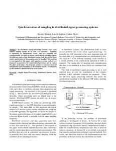
FIG. 1. Definitions of time of the signal and total delay. A : comparison between the peak time and the centroid 4, for a transient signal,f( t), with a shape of an a-function, i.e.,f( t) oc exp( - at). B: time delay is defined as the difference between the centroids of 2 transient signals. Here the total delay (TD), the delay between the input current and the resultant voltage response, is shown. t

l

x ty) =- Ri*tYl x eff R,

(9)

where X and R, correspond to the cylindrical branch in the direction of interest. Ri, in this expression is the input resistance of the structure at the direction of interest (substituting the boundary conditions in all other directions by sealed ends). When a steadv-state current is iniected at a given noint. the rate

DENDRITIC

DELAY

AND INPUT

of spatial attenuation of voltage at any point in the tree, is inverselyproportional to Aesin the direction to which the current is flowing. If we scale every infinitesimal small cylinder of electrotonic length dX by the corresponding Xeff(i.e., its new length will be dX X/X,,), we get a transformed representation of the structure. In this transform, each unit of distance represents an e-fold attenuation of steady voltage (see Brown et al. 1992 for a similar electrotonic representation of attenuation). 2) @@tive ~(r~,). Similarly, 7,ff extends the functional meaning of the conventional 7. Given a point y in a tree and a given direction, 7,ff is defined as the input delay (local delay) at that point, when the boundary conditions in all other possible directions are sealed-end conditions. As demonstrated in RESULTS (Fig. 217 ?eff = 7 in the caseof an isopotential structure. It is important to note that, in contrast to X,,, for 7effthe transmembrane direction is also a legitimate direction. For example, when the point y is at an isopotential soma that is coupled to a cylinder, two possible directions for current flow exist when 7effis considered: the flow through the soma membrane and the flow into the cylinder. For Xeff, however, only the latter direction is relevant. l

Theorems Several general theorems are used extensively in the following analysis of dendritic delay. Their complete proofs can be found in H. Agmon-Snir and I. Segev(unpublished data). THEOREM ~(SHAPEINVARIANCE). Thetotaldelaybetween any two points (y, x) in a given passivestructure is independent of the shape of the transient input current at point y. Clearly, this is true also for the LD(y) and the PD(y, x). THEOREMII(RECIPROCITY). Given two points (y, x) in an arbitrary passivestructure, TD( y, x) = TD( x, y). Note that this is not necessarilytrue for the propagation delay, PD. Note also that this theorem and the definitions for PD and NDD imply that NDD( y, 0) = PD(0, y). The velocity ofthe signal THEOREM III (VELOCITY THEOREM). depends only on the details of the structure in “front” of the signal. It is independent of the structure “behind” the signal and of the input point. The velocity of the signal at a given point, y, is given by Xe,( y)/ TeE(y), where XeR(y) , 7,& y) correspond to the direction considered. THEOREMIV(LOCALDELAYTHEOREM). TheLDatanypointy in the passive structure is the weighted mean of the input delays (i.e., of the corresponding 4 in the various possible directions from y. The weighting is by the corresponding input conductances. For example, consider the case of a point y along a finite cylinder. There are two possible directions (denoted by 1 and 2) for the signal at point y, one into cylinder 1 and the other into cylinder 2. The LD at y is

LD(Y) =

7eff,l

(Y)

l

Gin,l

(Y)

Gin,l(Y)

+ 7efT,2(Y)

+ Gin,2(Y)

l

Gin,2(Y)

(10)

where Gi,,l 7 Gin, 2 are the input conductances of cylinders 1 and 2,

respectively.

SYNCHRONIZATION

2069

Analytic techniques For computing delays in passive structures, we introduce a novel approach called “the method of moments.” In this approach the ith moment, mLi, of a transient signal,f( t ), is defined as mLi

=

ra0

tie f(t)dt

uo

J-co

Note that the centroid, $-,in Eq. 1 is exactly the ratio between the 1st and 0th moment. In general, it is possible to define other properties off(t), such aswidth, skewness,etc., by the use of moments. These properties of transients in passivestructures can be explored analytically by the use of the method of moments (unpublished data). To compute the delay in passive trees utilizing the method of moments, Rall’s one-dimensional cable equation was employed. The cable equation in dimensionless units (X = xl X, T = t/r) is - GT

V(X,

T) - V(X,

T) = -R;

I(X,

T)

(12)

By multiplying both sides of Eq. 12 by T’ and integrating over T, we get an ordinary linear differential equations with constant coefficients for each of the moments of the voltage response in a passive cable. These equations are very similar to the steady-state passive cable equation. For the 0th moment d2

For the ith moment, i = 1, 2, 3, . . . , d2 3

MY,i(X)

-

MVi(X)

= -R,*M,,i(X)

,

- i*Mvi-1(X),

(14)

where Mi.1 is the ith moment of the current input. Here the moments are defined over T. Using these ordinary differential equations (ODES) the moments can be analyzed by the same methods used in steady-state analysis of passive trees (Rall 1959, 1977). Note also that the equation for the ith moment depends only on moments of smaller or equal order. The equations for MVi in a given tree and a given transient input, I(t), can be solved analytically either directly or by using Laplace transforms. Some details are given in the APPENDIX, and complete treatment is given in H. Agmon-Snir and I. Segev (unpublished data). For the purpose of computing delays, only the 0th and 1st moment should be derived. Because any tree can be lumped into an equivalent “soma” ( Theorem V), it is sufficient to find the delay in the case of a cylinder coupled to a soma. As shown in the APPENDIX, the total delay in this caseis 2x

TD(Y, X) = ; + ; l (Y-L)*tanh(L-

Y)+$f$

- K’(l + 8 + L [ + ezx -T+

(15) K’(1

+f)-[*L

f - ezL

where 0 5 X I Y 5 L, and the soma is at the origin, X = 0. TD is expressed in units of 7d, and 4 =-

Pa,- 1 Pal +

1

(16)

Whenanalyzingdelays KZ- 72 - & in a structure, one can compute delays in any segment, replacing (17) Pa3 + 1 the structures (subtrees) at its boundaries by isopotential R-C compartments (“passive somas”), each has the same input resis- Utilizing the Reciprocity Theorem, replacing Y and X in Eq. 15, tance and input delay asthe corresponding original structure (sub- gives an expression for TD( Y, X) for the casewhere 0 5 Y I X5 L tree). This theorem is very useful for computing delays in arbi- (the input point is close to the soma and the recording point is trary trees by means of a recursive procedure (see below). distal to it). THEOREMV(EQUIVALENCETHEOREM).

2070

H. AGMON-SNIR AND I. SEGEV

As stated in Theorem V, any subtree in a dendritic structure can be lumped into an equivalent soma for the purpose of calculating delays. Hence using Eq. 15 and the theorems, the delays in arbitrary trees can be computed in each cylindrical segment separately, provided the input resistancesand input delaysat its boundaries are known. A recursive method, similar to the method developed by Rall ( 1959) for calculating input resistance and steady voltage attenuation, can be used here for calculating delays over such trees. This method was employed here to calculate the delays in Figs. 10 and 11 and in Table 1. For symmetrical trees equivalent to a single cylinder, a simpler method can be utilized (unpublished data). This method is similar to the method developed by Rall and Rinzel ( 1973) for calculating the attenuation of steady voltage in such trees. This method was employed here to calculate the delays in Figs. 8 and 9. RESULTS

The analytic solutions provided by Eq. 15 and Theorems I-V above enable one to explore the velocity and time delay of signals propagating in passive structures. In the following we start to analyze simple structures and progressively add complications until realistic trees are encountered.

A

Local Delay = T

1.v

B t-------x-

Local Delay = 2/2 Velocity = ~-I/T

Two simple cases DELAYINANISOPOTENTIALCELL. Inthelimitingcase,when

L in Eq. 15 approaches 0, the delay in an isopotential cell is obtained. In this case the voltage response lags in time behind the current by exactly T, the time constant of the membrane (see also Rall 1967 ). This LD reflects the time course for charging the membrane capacitance (Fig. 2A). DELAYINSEMI-INL~NITEANDINL~NITECYLINDERS. Thelimiting case, L --t co and p, --* cc, in Eq. 15 corresponds to the delay in a semi-infinite cylinder with a sealed end. When the recording point, X, is set to 0 (the sealed end), the TD between an injection point Y and the point 0 is simply ( 1 + Y) - 7/ 2. The reciprocitytheorem(Theorem II) implies that when the current is injected at the sealed end (Y = 0) and the recording is at point X, the TD between these two points is ( 1 + X) * ~/2 (Fig. 2B). This then gives two important results. 1) The LD at the sealed-end boundary of a semi-infinite cylinder is T / 2, one-half the delay in an isolated soma with identical membrane properties. In the semi-infinite cylinder the LD is smaller because of the loss of charge from the injection point to other regions of the cylinder. The rate of this loss is faster than the rate by which charge is lost through the membrane (Rall 1969). It is easy to see from the local delay theorem(Theorem IV) that ~/2 is also the LD at any point in an infinite cylinder. 2) The PD between the sealed end and point Y is Y. r/ 2. The signal velocity, 8, is therefore 2 . X/T. This is also the velocity at any point in an infinite cylinder. It was previously shown that 2. X/T is the asymptotic value for 0 in infinite cylinders when other definitions for the time of the signal were used (Jack et al. 1975 ) . We note that the velocity can be calculated alternatively from the velocitytheorem that states that the velocity is the ratio between X,, (which is simply X in this model) and the T,~ (which is the LD, T / 2 ) . In this case the ratio is 2. X/T.

FIG. 2. Local delay (LD) in 2 simple cases.A : in an isopotentialcell, the LD (alsothe TD) is exactly7, the time constantofthe membrane.B: in a semi-infinite cylinder,the LD at the sealedend (“electrode” I) is only r/2. The velocityof the resultantvoltageresponse(V) at any point in the direction ofthe infinite extension(heavyarrow) is 2X/r. Theseare alsothe LD and velocityat any point in an infinite cylinder.The TD betweenthe input point at the sealedend and the recordingpoint is ( 1 + X) . r/2, and this is the TD betweenany 2 points in an infinite cablewhosedistanceis X.

Finite cylinder with both endssealed The limiting case p, + co in Eq. 15 corresponds to the delay in a finite cylinder with both ends sealed. The TD between an injection point, Y, and the recording point X, OSXS Yisthen TD=‘/2.[1

+L.coth(L)-X.tanh(X) -(L-

Y).tanh(L-

Y)]

(18)

From this expression the LD and the signal’s velocity as well as the PD in this model can be computed. LD. Figure 3A shows a cylindrical cable whose electrical length is L and an “electrode” injecting a transient current I at point Y, and recording the resultant voltage Vat that same point. Figure 3 B depicts the LD in such finite cylinders of various lengths. As expected, LD in short cylinders (e.g., L = 0.5, L = 1) is close to T, the LD in an isopotential structure. In very long cylinders (e.g., L = 8)) however, LD at both ends as well as in the middle of the cylinder is close to 7/2, the value obtained in infinite cylinders. The figure also shows that, as expected from the local delay theorem, LD at each end of a cylinder of length L is equal to LD at the middle of a cylinder of length 2 L. In general, the LD in finite cylinders with both ends sealed is always between 7 / 2 and T. It is worth noting that in short cylinders the LD is maximal at the middle of the cylinder, whereas in long cylinders a local minimum is obtained at that point. This is demonstrated in Fig. 3C, where the loci of the local max-

DENDRITIC

DELAY

2011

AND INPUT SYNCHRONIZATION

A

B

2 0.8 8 YX

L=2.0 L=8.0

i1.:: '012

L (V

3

4

56

7

8

y (V

FIG. 3. LD in a cylinder ( 2 sealed ends). A : schematic drawing of the model used. A transient current (I) is injected, and the resultant voltage (I’) is recorded at a point Yin a cylinder whose electrical length is L . B: LD as a function of the injection point Y is shown for cylinders with L = 0.5, 1.O, 2.0,4.0, and 8.0. C: locations of maxima in LD are shown as a function of the cylinder length. D: dependence of LD on both Y and L is shown. Note that in this case the LD is always between r and

T/2.

ima are shown as a function of the cylinder length. For cylinders shorter than -2.5X, there is only one maximum. In longer cylinders the bifurcation in the graph shows that two local maxima exist, one in each half of the cylinder. The complete picture is shown in Fig. 3 D , where the local delay is plotted as a function of both the cylinder length L and the injection point Y. The result of Fig. 3 B that demonstrates an increase in LD as the electrode moves away from the boundary is somewhat surprising and requires an explanation. This can be done considering, once again, a semi-infinite cylinder and the local delay theorem. When the injection point is at the sealed end, the LD is 7 / 2. When the injection point moves slightly from the sealed end, say by 0.1 X, a short cylinder is practically added at one side of the electrode, whereas the other (infinite) side remains essentially unchanged. This short cylinder is almost isopotential; it therefore has a large input delay of approximately T (see Dejinitions) and, although this cylinder may contribute very little to the LD, it must elevate the LD beyond T / 2. When the injection point is moved far from the sealed end, the cylinders at both sides of the electrode are electrically long and, thus the LD is, again, close to r / 2. Therefore in semi-infinite cylinders the LD as a function of the injection (and recording) point is expected to first increase to a maximum and then decreases asymptotically toward ~/2. For long, but finite, cylinders

the same behavior can be seen near both ends of the cylinder (Fig. 3B).’ SIGNAL VELOCITY AND PD. From the velocity theorem it is easy to derive an expression for the velocity ( fl) of the signal at a point X, when the signal propagates toward the origin of the cylinder (Fig. 4A). As noted above, 0 = X,,/ T,~. Here XeE= coth(X)and,fromEq. I~,T~~= (1 +X.[coth(X)tanh(X)]}/2. As can be seen in Fig. 4A, the velocity approaches 2. X/T for large values of X (dotted line), as expected. When X is close to the origin, the velocity increases and approaches infinity when X --, 0, as expected near a sealed-end boundary (Goldstein and Rall 1974; Jack and Redman 197 la,b; Rall 1967; Segev 1990). Note that the velocity at point X is dependent neither on the cylinder length L nor on the point of injection Y (provided that Y 2 X). If we observe Fig. 4A it is surprising to find a local minimum (a “dip”) in the velocity curve near X = 1. This ’ An alternative interpretation of the behavior of the LD is that the injected charge accumulates at the short cylinder that was added. As a result, the voltage at the injection point remains large for longer times, thus broadening the voltage response and delaying the centroid. Interestingly, our theoretical and numerical studies show that, when the injection point in a finite cylinder with sealed ends is off the cylinder’s center, the site of voltage peak moves in time from the injection point toward the sealed end. When the peak arrives to the end, this end becomes the current source.

2072

H. AGMON-SNIR

_A _

AND I. SEGEV

B

10 II

d _______--------..... s OO 2 ,----k ---.__ 1 --a------------.-.-.-.-.-.-2 3 .------4

heff 5 Zeff

x (U

C E

1.5.

0

A

L=l.O

0.8

E

I 0

0.25

0.5

0.75

1

x (V FIG. 4. Velocity and delay in a cylinder (2 sealed ends). A: velocity of a signal propagating toward a sealed-end origin (heavy arrow). For comparison, the function “y = 2,” the velocity in a control case of an infinite cylinder is drawn by the dotted line. Note the slight deceleration around X = 1. Dashed and dot-dashed line depict )Ls and r,s, respectively, for a signal propagating toward the sealed end. B: propagation delay (PD) between a point X to the origin. The function “y = x/ 2” is plotted by the dotted line. C: TD between an injection point Y and the cylinder origin at point 0 is depicted for 3 cylinders with L = 0.5, 1.O,and 2.0. Note that the end-to-end delay is larger than 7 for any L value. D: TD( Y, X) is shown for 10 injection points (Y = 0.1,0.2, . . . , 1.O), in a cylinder with L = 1.O. Dashed curve is the LD for this cylinder.

reduction in 0 is a result of two opposing factors that affect the velocity: when X is decreased, T,~ ( dot-dashed line) gets larger (charge accumulates near the sealed end), tending to broaden the voltage transient thereby decreasing the velocity. At the same time, X,, (dashed line) increases (smaller attenuation near the sealed end), tending to increase the velocity. Next, the PD between any two points, Xi, X, (Xi I X,), when the signal is moving toward a sealed end is analyzed. Because the PD between X, and X, is PD (X, , 0 ) - PD (X, , 0 ) , it is sufficient to analyze PD between X to 0 (continuous line in Fig. 4B). Note that here, again, PD(X, , X,) is dependent neither on the cylinder length L nor on the point of injection Y (provided that Y 2 X, 2 Xi ) . The dotted line shows PD(X, 0) when the boundary condition at point 0 is equivalent to an infinite cable extension. In the latter case the PD (in units of T) is precisely X/2. If one compares the two curves, one can see that they differ only near the origin but that they do converge at large X values. As an result, for large X, PD(X, 0) in a cable with a sealed end at X = 0 is very close to X/2 (in units of T), in spite of the change in the signal velocity when propagating toward the origin. TD. To conclude the discussion on the delay in finite cylinders with sealed ends, the TD in this case is shown in Fig. 4,

C and D. In C the TD between an injection point Y and the sealed end at the origin is depicted by the continuous lines for three cylinders with L = 0.5, 1,2. There are two points to note. First, the TD from one end of a cylinder to the other is always larger than 7. Namely, compared with an isopotential structure where the TD (which is also LD) is r, the TD increases in the cylinder when the signal propagates between its two ends. Nonetheless, cylinders allow for faster communication (smaller delays than 7) for some values of X < L. This communication can be much faster in dendritic trees (see below). Second, Fig. 4C shows that, as is the case for the LD (Fig. 3 ), the TD from one end to the other in a cable of length L is equal to the TD from the middle of a cable of length 2L to each end. Finally, in Fig. 40 the TD( Y, X) is shown for 10 injection points (Y = 0.1 X, 0.2X, . . . , 1X) in a cylinder with L = 1. The dashed curve depicts the LD for this cylinder. Because the velocity is independent of the injection point, all curves have parallel slopes for each value ofX. Again, when the injection point is at the other end (Y = L = 1 ), the TD is larger than 7. When Y < 0.4 (4th line from bottom), TD < 7. CYLINDER COUPLED TO A SOMA. This section treats a more general case of a cylinder where at one end the cylinder is sealed (at point L) , whereas at the origin (X = 0) the cylin-

DENDRITIC

DELAY

AND INPUT

’

SYNCHRONIZATION

/4-L

0.8

/ 0 (e-,I He

B l-l : 0.4

I/

----..--y=o.5 -----Y=1.0

__---__-----

&=l L=l

-T.Delay(to --L.Delay

I

o.oo

2073

1

2

3

X=0) 4

5

FIG. 5. Velocity and delay in a soma + cylinder model (uniform R,). A: schematic drawing of the model. A passive soma is coupled to a cylinder with the other end sealed. L, cylinder length, Y, injection point; X, recording point. In this figure, uniform membrane is assumed ( 6 = 1) . B: velocity of a signal propagating toward the soma for pm= 0. 1, 1, \12,and 3. C: TD (Y, X) when the injection point (Y) is at the sealed end (Y = L = I), plotted as a function ofX. D: TD to soma (-) and the LD ( - - -) are plotted as a function of pm for 2 injection points (Y = 0.5, 1) and a cylinder with L = 1.

der is coupled to an isopotential passive soma (Fig. 5A). Note that, as stated in Theorem V, for the analysis of dendritic delay, the boundary condition imposed by any passive structure at the end of a cylinder is equivalent to a boundary condition of an appropriate soma. This will be used later when more complicated dendritic models are treated. Two parameters, p, and t, are used to uniquely define the boundary condition at the soma end. In Fig. 5, B-D, the soma membrane and the membrane of the cylinder have the same time constant, namely E = 1. The velocity of a signal propagating toward the soma is shown in Fig. 5 B, for four various values of p, (0.1, 1, 1(2, 3). For a fixed c, a larger pm value corresponds to a smaller soma. First thing to note is that, depending on p, , there are three domains of velocity behavior. For pm < 1, the velocity first increases then decreases as the signal propagates toward the soma. For 1 < poo < d2, the velocity decreases monotonically, whereas for p, > v2 the velocity first decreases then increases. For a small (large p,) the qualitative behavior is as expected near a sealed end (Fig. 4A ) . A large soma has two opposing effects. At distal points the soma acts as a current sink, thereby enhancing the decay of the voltage transients at these points as compared with the infinite cylinder. This narrowing of the voltage transients becomes more significant as the signal propagates toward the soma; hence the

velocity increases. On the other hand, when the signal approaches the proximity of the soma, another effect becomes dominant. At the large soma, charge accumulates (and decays) slowly relative to the points near the soma; hence the velocity at this region decreases. Between these two extreme cases, the effect of the soma is to decrease the velocity at all points. Another finding is that the velocity near the soma (in units of X per T ) approaches the value of p, . This can be easily seen by the use of the velocity theorem and the definitions to X,e and T,~. In Fig. 5C the total delay from an input at the cylinder end to various points is depicted. In the case shown, L = 1 and E = 1. If we focus on the TD from the distal end to the soma (X = 0), the figure shows that the presence of soma increases this delay as compared with the case without soma (where p, = co). The TD increases as pm decreases. This can be shown to be true for any L and Y. Also, this relation between TD( L, 0) to p, agrees with the behavior of the velocity near the soma, where an increase in p, is associated with a increase in the velocity near the xoma (Fig. 5 B). Changes in velocity far from the soma, on the other hand, seem to be less dominant in determining the TD to the soma. In Fig. 5 D the dependence of the TD( Y, 0) ) and the LD (- - -) on p, can be appreciated. In (-general, as the soma size increases (i.e., pm decreased), the value of TD( Y, 0) increases, and the value of LD at any

H. AGMON-SNIR

2074

AND I. SEGEV

A 8

C 1.25

&=0.25

Y=l.O

L=Y=l

Y=O.5

1.6

;

0.25.

0

0.2

0.4

0.6

0.8

1

x (A)

h 1.2 rd ri

Y=O.5

'

Y=l.O

0.8

u.4.

0

0.5

1 &

1.5

2

6. Velocity and delay in a soma + cylinder model (nonuniform R, - shunt soma model). Same model as in Fig. 5.4, but here various c values are explored. Velocity of a signal propagating toward the soma is shown for various values of c = 0.5). C: TD when the injection point is at the sealed end is plotted as a function of X, for e = in A (Pm = 2)andinB(p, 0.25 and various values of poo. D: linear dependence of TD (-) and local delay (- - -) on c is demonstrated. FIG.

point Y # 0 decreases. If one observes the TD from end to soma (Y = 1 ), one finds that it is bounded between 1.2 and 1.4. Thus, in this case, the TD depends rather weakly on the value of poo. In contrast, the LD at Y = 1 is greatly influenced by poo (and, consequently, also the PD). For any fixed value of poo, when the injection point is closer to the soma ( e.g., Y = 0.5 ) , the LD is larger than at Y = 1, whereas the TD is smaller. To conclude, unless the cylinder is very long, the TD from end to end is of the order of 7. To complete the analysis of a soma lumped to a cylinder, the case with E # 1 (i.e., 7, # Q) is depicted in Fig. 6. The velocity of a signal propagating toward the soma is shown for various values of E for pm = 2 in A and for poo = 0.5 in B. These graphs should be compared with Fig. 5 B. Again, it can be proven that the velocity near the soma end (in units of X per TV) approaches the value of p&. For this more complicated case, four types of velocity behavior are observed. Depending on pm and on c, the velocity may first increase then decreases (e.g., Fig. 6B, c = 0.2); it may first decreases then increases (e.g., Fig. 6A, f = 0.5); it may decrease monotonically (e.g., Fig. 6A, E = 2) or increase monotonically (e.g., Fig. 6 B, c = l/16). It can be proven that near the soma the velocity increases for ( p, )’ > 2 E and decreases for ( pm)2 < 2 E. Figure 6C shows the TD (in units of TV) from Y to soma for the same model as in Fig. 5C, except that, here, E = 0.25. l

l

In contrast to Fig. 5C, here the TD( Y, 0) increases as pa increases. This relation between TD to the soma and pm fits the behavior of the velocity at distant locations from the soma where an increase in poo leads to a decrease in the velocity. Changes in velocity near the soma, in this case, seem to be not significant in determining the behavior of the TD to the soma. In general, it is possible to show that if c 1 the TD behaves as in Fig. 5C. When 1 > c 2 0.5, the behavior depends on L . For long cylinders, the TD behaves as in 5C. It is important to note that the behavior of TD does not depend on Y. Opposite to the results with 6 = 1 (Fig. 5C), in Fig. 6C the TD from end to end is shorterthan the TD in a corresponding cylinder with a sealed end at X = 0 (where theTDz 1.2forL= 1). Namely, when the sealed-end boundary conditions are replaced with a shunted soma, the communication speed along the cylinder can be enhanced (the delay can become smaller). To complete this analysis, Fig. 60 shows the dependence )andtheLD(---),onc.Itcanbe of the TD (Y, 0) (proven that the dependence of the TD on Eis always linear; the slope depends on L, X, and poobut not on the injection point Y. As expected, the effect of increasing 7, (and therefore increasing E) leads to an increase in all the three types of delay. It is evident from this figure that LD, TD, and PD depend strongly on c.

DENDRITIC

r 0

-1 x od

DELAY

AND INPUT SYNCHRONIZATION

2075

2

1 x w

C Lo=1 L1=-

Y=l

-G 2 l-l I!? r-l :: I2

1

1 -0.5 0 0.5 0.5 x (hl) x (M x (ho) x (W FIG. 7. Velocity and TD in a cylinder with step diameter change. A : inset shows model of a cylinder with a step diameter change. Distances are measured with respect to point of diameter change (X = 0). Units are in X0 for the prestep cylinder and in X, for the poststep cylinder. L, and L, are the electrotonic lengths of the corresponding cylinders. 6 = d, /d,, where d, is the diameter of the poststep cylinder and do is the diameter of the prestep cylinder. In A the velocity of the signal propagating from the injection point Y is shown for L, = cc and various 6 (4, 2, 1, ‘12, Ilq). The velocity is given in units of X0/7 for the prestep cylinder and X,/T for the poststep cylinder. The velocity in poststep cylinder is constant, 2X, /T. B: TD( Y, X), when both cylinders are infinite. Note that in this case the TD to the step change TD (Y, 0) is independent of the value of 6. C: TD when the prestep cylinder is finite and the poststep cylinder is infinite. D: TD when the poststep cylinder is electrically short (L, = 0.5). -0.5

0

Cylinder with a step change in diameter In this section we are interested in the behavior of the signal when it passes through a step change in the cylinder diameter. For the present analysis, the step change is at X = 0, and the signal moves from right (where the diameter of the prestep cylinder is d,) to left (where the poststep diameter is d, ; inset in Fig. 74. The ratio d, /d, is denoted by 6. Units are in X, for the prestep cylinder and X, for the poststep cylinder. L, and L, are the electrical lengths of the corresponding cylinders. Rall ( 1959) has proven that this case is equivalent to a branch point at X = 0, where do is the parent branch and d, i are the daughter branches such that (d,/dO)3’2 = Zi [ (do i /d,) 3/2] and all daughter branches have the same L value (and same boundary conditions) as the original, poststep, cylinder. First, we analyze the case of a step change in a cylinder that extends infinitely at both ends (Fig. 7, A and B). In A the velocity of the signal (in units of X/ 7, where X corresponds to the respective cylinder) as it propagates to the

1

step change (X = 0) and beyond is depicted for various values of 6. It is not surprising that velocity in the prestep cylinder behaves qualitatively as in the model of a cylinder coupled to a soma (Figs. 5 and 6). Indeed, it can be shown that in this case the effect of the poststep cylinder on the delay at the prestep cylinder is equivalent to the effect of a soma with c = l/2and poo = ( do/ dl ) 3/2. A consequence of the velocity theorem is that the signal propagates at constant velocity, 0 = 2. Al/7 = 2 X0/7. VS, from the step change further down along the poststep cylinder. An interesting result is shown in Fig. 7B, where the TD as a function of X is depicted. It demonstrates that the TD from the injection point to point of step change in diameter is independent of 6; i.e., the acceleration and deceleration of the signal exactly compensate each other. The mathematical proof is simple: reciprocity theorem implies that TD from the injection point Y to point X = 0 is equal to the TD in the reverse direction. This TD is the sum of the LD at point X = 0 and the PD (0, Y). At the junction point of two semi-infinite cylinders, the LD is always 7 /2. Because the l

2076

H. AGMON-SNIR

PD does not depend on the structure “behind” the signal, it does not depend on d, . That concludes the proof that TD is independent of 6. This result is valid for any injection point Y. When the prestep cylinder is finite and the poststep cylinder is infinite, then TD( Y, 0) increases as 6 decreases ( Fig. 7C). This agrees with the results for the soma-cylinder model, with c = ‘12(see above). Namely, the net effect of a decrease in diameter ratio of the two cylinders is to slow down the propagation of the signal when it approaches the step change. This is not necessarily the case when the poststep cylinder is finite. The input delay of this cylinder might increase toward 7 and then, similar to Fig. 5C, TD( Y, 0) may increase rather than decrease when 6 increases (Fig. 70). Trees equivalent to a single cylinder In this section the delay in idealized dendritic trees is analyzed. Although our method can be implemented on arbitrary passive trees, many important insights can be obtained from analyzing the family of trees that are equivalent to a cylinder (Rall 1959, 1962a,b, 1969). Rall and Rinzel ( 1973) introduced an analytic method to compute the attenuation of steady voltage in such trees, with current injected to only one dendritic branch. The same idea was also employed here for the investigation of signal delays in such trees (unpublished data). An example of the classical results of Rall and Rinzel concerning steady-state voltage attenuation in idealized trees is depicted in Fig. 8A. The modeled tree is schematically shown in the inset. In A a steady current (I) is injected at the tip of the lower terminal ( T, ) of a tree consisting 3 order of (symmetrical) branching, each branch is 0.25X long (i.e., total length L = 1). In this case there is no soma (P = a ). The continuous lines show the voltage attenuatio”n along the tree. Although all branches have the same length, the voltage attenuates most steeply along the input branch and less steeply along the more proximal branches. For comparison the steady attenuation in the equivalent cylinder, when the current is injected at L = 1, is shown by the dashed line. Note that at the origin of the tree (X = 0), the voltage responses in the full tree and in the equivalent cylinder are the same. It is worth noting that Fig. 8A also shows the attenuation of the area under the voltage response when a transient (rather than a steady) current is injected at the same tip (Rinzel and Rall 1974). Figure 8B shows the TD along the same tree for a transient current injected at T, (continuous line). The dashed line depicts the TD in the equivalent cylinder. Numbers denote PD over individual branches. First note that, if we observe the four branches on the path from tip ( T, ) to origin, the delay in the second branch (0.32) is larger than the delays in all other branches. Also, the velocity decreases as the signal approaches a branch point and increases immediately after that point. This behavior is well understood in view of the results obtained for the soma-cylinder model and the step diameter change model. The TD from T, to origin is - 1.2; this is also the TD for the equivalent cylinder. The LD at T,, however, is smaller than the LD at the

AND I. SEGEV

corresponding point in the equivalent cylinder. This figure demonstrates that the delay to various possible “target” points in the tree may differ significantly. This delay (and the communication speed) is not only a function of the distance from the input point to the target point but also a function of the morphology between the two points (e.g., compare the TD with the 2 points that are 0.5X from T, ). The effect of a soma on the TD in a tree is demonstrated in Figs. 8, C and D. In C, c = 1 (uniform R,). Compared with Fig. 8 B, the TD to the origin increases, as expected. In contrast, the LD at T, decreased and, thus the PD( T,, 0) increased. Interestingly, along the path from T, to the soma, the PD over the first two distal branches decreased (0.2 1 and 0.30 compared with 0.27 and 0.32, respectively), whereas the PD over the two proximal branches increased. The TD from T, to the other dendritic tips ( T2, T3, and T4) decreased because of the presence of a soma. Finally, the effect of a leaky soma is examined in Fig. 8 D. In this example the membrane resistivity of the soma was reduced IO-fold, keeping the soma dimensions as in C; hence both c and poo were reduced by a factor of 10. As a result of the somatic leakage, the delays to any point in the tree were reduced in comparison with the corresponding points with nonleaky soma. DISCUSSION

The present study introduces a novel analytic approach to analyze transients in passive structures with special focus on synaptic potentials in dendritic trees. The underlying idea is to characterize the various properties of the transient signal (i.e., its area, its center of gravity, its width, etc.) with the use of the signal’s moments. Utilizing Rall’s cable theory and the definitions for the moments, one can write a system of linear ODES that describes the behavior of the various moments as the signal spreads in the dendritic tree. These equations can be solved analytically for passive trees with arbitrary branching pattern and arbitrary spatiotemporal distribution of current inputs. This method is general and might prove applicable to the analysis of transients in various electrical circuits such as bipolar chips, for example. It is important to stress that, although the analytic results of the present study hold for any transient (provided that the integrals for the moments in Eq. II exist and the 0th moment is not 0), the use of the centroid (and the definition of delay) is meaningful essentially to predominantly monophasic transients, as most synaptic currents and potentials are. A particular application of this “method of moments” is the analysis of time delays in passive dendritic trees. Here only the first two moments, the 0th and lst, are used to define the centroid (center of gravity) of the transient involved (the transient current input or the transient voltage response). Delay and velocity are defined with respect to the centroid. Namely, we describe how the centroid (as distinguished from the peak) moves in time along the modeled tree. Several important theorems regarding the signal delay and velocity in passive trees are stated, and an efficient recursive algorithm for calculating the delay and the velocity in realistically complex dendritic trees was developed. The

DENDRITIC

DELAY

AND INPUT SYNCHRONIZATION

2077

A 1

41

a, b

!?

0.8

0.24

T4

I T3

0.6

I T2 T2

0.4:

2

T3 T4

0.2: VP-

0

0.25

C

0.5

0.75

1

0.25

X(h) 1.4; T4

G V

2 f-i E

Tl

1: T3

0.8:

0.5 x (V

- 1.4: 2 1.2: 1; 2 l-i a, 0.8;

a

T4

"m 0.6:

4

g 0.4:

2 0.4

T3

E-l 0.2

T2

0.2' cOt

0.25

0.5

0.75

0.6

1

cO

x0

Tl

0.25

0.5 x (U

0.75

1

FIG. 8. Trees equivalent to a single cylinder. The model is an idealized tree with a total electrotonic length of 1. Each branch is 0.25X long. Current is injected at a distal tip T, ( inset). A : classical result showing steady voltage attenuation over the tree (after Rall and Rinzel 1973). For comparison, the attenuation for the case of input at the end of the equivalent cylinder is shown by dashed line. The same method of demonstration is used in B-D for the delays in such a tree. B: TD between the input point to any point in the tree. For comparison, TD when current is injected at the end of the equivalent cylinder is drawn by dashed line. Numbers denote PD over branches. C: effect of a soma that has the same membrane time constant as the tree (E = 1). D: as in C but with a shunted soma with a lo-fold decrease in soma R, (6 = 0.1).

proofs for these theorems and the details of the algorithm are given elsewhere (H. Agmon-Snir and I. Segev, unpublished data). A further application of the method of moments to explore analytically the behavior of the signal’s width (defined using Oth, 1st, and 2nd moments) and skewness (using also the 3rd moment) is in progress.

properties of the membrane and is exactly 7. This reference case gives an upper limit for the LD in passive dendritic trees because in distributed (nonisopotential) systems the input current can be discharged both through the membrane at the input site and also longitudinally to other regions of the tree. Therefore a more rapid discharge of the

Local delay-LD The LD at a given input point reflects the RC properties of the membrane and the electrotonic structure of the dendritic tree as “seen” from the point concerned. It can be interpreted as a measure for the width of the time window in which the local voltage response at the input point is significant. In the context of electrical communication between adjacent synapses, the LD is an indication of the “life-time” of local synaptic potentials; i.e., the local time window for nonlinear interactions between synaptic excitation and synaptic inhibition (Segev and Parnas 1983). Therefore it is a measure for the degree of synchrony required for these synapses to interact locally; small LD implies that inputs have to be well synchronized to interact with each other. In the reference case of an isopotential system, the input current can be discharged only through the membrane. Indeed, the LD as defined here using the centroid reflects the

Order

of

branching

9. LD in a terminal tip of an idealized dendritic tree as a function of the order of branching. LDs for idealized symmetrical trees with L = 0, 5, 1, and 5 are drawn. Note the sharp decrease in LD for the electrically short trees (L = 0, 5, 1) when the order of branching increases. Inset: the case of a symmetrical tree with 3 orders of branching. FIG.

2078

H. AGMON-SNIR

input current is expected with the result of a reduced local delay associated with a briefer voltage response at the input site as compared with the isopotential case (Rall 1967, 1969; Rinzel and Rall 1974). A useful reference case for such distributed systems is the cylinder of infinite length. Here the infinite extension of the cylinder serves as a sink for longitudinal current spread from the input site, and the well known response function for this case decreases the LD to exactly 7/2, namely one-half that for the isopotential case. With an addition of a soma at one end of the cylinder and in the presence of a dendritic tree, the LD at certain dendritic locations, typically at distal arbors, may become very small (e.g., 0.17), because the rest of the tree serves as a large current sink. Other, more proximal locations in the tree may undergo very different LD, of the order of 7 (as in an isopotential soma). As a general rule, LD at distal dendritic arbors decreases as the complexity of the tree increases. This is demonstrated in Fig. 9 for symmetrical trees. For any fixed L value, an increase in the order of branching is associated with a decrease in the LD at the input tip. The decrease is marked for electrically compact dendrites (0.5 < L < 2) and with branching order of three or more, as found in many neuron types. For example, in the case of L = 0.5, with three orders of branching (as depicted by the schematic inset), the LD at the terminal tip is rather large (0.67). It decreases to 0.0777 when the order of branching is eight. The latter case could be relevant to parallel fiber inputs impinging on distal dendrites of cerebellar Purkinje cells that typically bear only one tree with an L value estimated at -0.5 and a branching order of S- 10 (Rapp et al. 1994). A LD of the order of 0.17 is also expected in distal basal and apical tips of cortical pyramidal cells (Fig. 10). A similar, and possibly smaller, LD (associated with briefer voltage transients) is expected at terminal tips of cat cu-motoneurons that typically bear several stem dendrites each having 10 orders of branching or more (R. E. Burke, personal communication). From the analysis of Figs. 8- 10, we can conclude that the branching order is a very important factor in reducing the LDs at distal dendritic arbors. As noted above, a small LD is associated with a brief (narrow) voltage transient at the input site (see also Rinzel and Rall 1974). The implication is that for local dendritic processes (e.g., plastic changes at the dendrites that are triggered by the local voltage transients) the exact timing (synchronization) between adjacent distal inputs is very critical. For example, the N-methyl-D-aspartate (NMDA )-based long-term potentiation (LTP) in the hippocampus depends critically on input timing. This input is believed to be the (brief) non-NMDA conductance change that impinges on distal dendritic spines (Brown et al. 1988). Total delay- TD The TD from an input point to a target point reflects both the rise time of the voltage response at the target point as well as the width of the time window in which this response is significant. This results from the use of the centroid (which depends on both the rise time and the decay of

AND

I. SEGEV

the voltage response) for the definitions of delays. As discussed below, in most interesting cases the rise time is small compared with the width of the time window. Hence, in the context of electrical communication between a synapse and the target point, the TD is practically the “life-time” of the synapse voltage response at the target point. A main result of the present study is that, in trees with electrotonic length of - 1X, the TD to the soma is typically on the order of 7. For proximal dendritic inputs the TD to the soma may be somewhat smaller, whereas for inputs at distal tips the TD to the soma (or to other dendritic trees) may be somewhat larger than 7 (see Figs. 8 and 1OA and Table 1). Note that this is true only for the uniform R, model of Fig. 1OA. For a shunted soma model (Fig. 10B) where the dendrites have a large R, value (and therefore large local membrane time constant), the TD may be more than three times the slowest (system) time constant (Q). Because the range of delays between the dendrites and the soma is on the order of 7, the exact synchronization of the various inputs is less significant than is the synchronization for the local interactions in distal dendritic arbors. However, as Rall ( 1964) first suggested, dendritic-to-soma delay and spatiotemporal input distribution may still be very important for the computations performed by the nervous system (e.g., for computing the direction of motion). Comparing the “life-time” of signals in global interactions (e.g., at the soma) with the “life-time” of the signals in local interactions at distal arbors, one can conclude that in local interactions the decision point functions more like a coincidence detector, whereas in global interactions the decision point functions more like an integrator (see also Softhy, 1993). In the context of actually computing the TD, the reciprocity theorem (Theorem II) is very useful. Because the TD (but not the PD) from any dendritic site(s) to the soma can be computed by injecting the current into the soma and measuring the voltage response at the site (or sites) of interest, a single run (with a somatic input) is sufficient for computing the delay from all dendritic locations to the soma. Finally, the effect of dendritic spines should be discussed. In many types of mammalian CNS neurons, including cortical pyramidal cells such as the one in Fig. 10, dendritic spines make up a significant fraction of the dendritic membrane area (capacitance). Spines were not included in the computations for Fig. 10 and Table 1. To examine the effect of spines on our results, Table 1A was recomputed, this time assuming that spines are uniformly distributed over the dendritic surface and that they add a total of 33% to the dendritic membrane area of the modeled cell. Spines were incorporated globally into the model with the use of the method of Holmes ( 1989; and see also Rapp et al. ( 1992). For the present case the membrane area of the spines is effectively added to the modeled dendrites by decreasing the dendritic R, by a factor of 2/3 and by increasing Cm by a factor of 3/2. This effectively increases the cable distance between any two (anatomic) points in the tree without changing the membrane time constant. Thus the TD between any two points is expected to increase when spines are added. Indeed, for example the TD from point 1 to the soma is 38.9 ms with spines instead of 34.2 ms without

DENDRITIC

DELAY

AND

INPUT

SYNCHRONIZATION

2 Local Delay = 2.4 ms Delay to soma = 28.2 ms

2079

2 Local Delay = 6.0 ms Delay to soma = 45.4 ms

-1

-1

fi’cm Local Delay = 12.4 ms Delay to soma = 62.0 ms

Local Delay = 4.6 ms Delay to soma = 34.2 ms

R md= 53,000 R ms= 900 Qcm* Ri = 336 Qcm c m = 0.9 pF/cm*

R,= 20,000 Q-cm * Ri = 100 Q-cm 1 pF/cm* Cm=

/

100 pm

100 pm

I

, Soma

, Soma

al Delay = 16.4 ms

:a1 Delay = 18.0 ms

3 Local Delay = 33 ms Delay to soma = 20.9 ms

3 Local Delay = 2.6 ms Delay to soma = 19.5 ms

FIG. 10. LD and TD to soma in a reconstructed pyramidal cell from layer V in cat visual cortex. Input locations are marked by arrows. Points 1 and 2 are at tips of the apical tree and point 3 is at a tip of the basal tree. Computations were performed with 2 different setsof biophysical parameters. In A, the uniform R, model is utilized, whereas in B a nonuniform R, (shunt soma) model is used. The corresponding specific values are given in the figure. Parameters for the shunt soma model in B were taken from Stratford et al. ( 1989). In case B the slowest (system) time constant, TV, is -20 ms. Morphological data were kindly provided by R. Douglas.

spines (Table 1A ); the TD( 1,2) is now 40.2 ms rather than 34.6 ms. Propagation delay ( PD) and the net dendrites delay ( NDD) Next, it is important to explore the net effect of the dendrites in delaying voltage signals. Both the PD and the NDD were defined for this purpose. For computing the PD from point y to the soma (0), the local delay at y is subtracted from the total delay to the soma (0), whereas for computing the NDD, the local delay at the soma is subtracted from the total delay to the soma. Thus PD is a measure for the propagation time of the voltage centroid from the input site to the soma. The NDD measures the “delay TABLE

1.

cost” that results from placing the input at the dendrites rather than at the soma. Because of the reciprocity theorem ( Theorem II), TD(y, 0) = TD( 0, y), and we get a remarkably simple relation between these two measures 0) = PW, Y) WV In general, because the LD at the soma is typically larger than the LD at any dendritic site, the PD( y, 0) is expected to be larger than the NDD( y, 0). In the case of an input to a distal apical dendrite (e.g., point 1 in Fig. IOA) the PD is quite significant (34.2 - 4.6 = 29.6 ms); for the input to the basal dendrite (point 3 ), this delay is smaller but still significant ( 19.5 - 2.6 = 16.9 ms). The corresponding values of the NDD are smaller, namely 34.2 - 18 = 16.8 ms ( -0.87) NDWY,

Delays in the pyramidal eel/ models shown in Fig. 10 A. Uniform Membrane Model

Soma 1 2 3

B. Shunt Soma Model

Soma

1

2

3

18.0 34.2 28.2 19.5

34.2 4.6 34.6 35.6

28.2 34.6 2.4 29.7

19.5 35.6 29.7 2.6

Soma 1 2 3

Soma

1

2

3

16.4 62.0 45.4 20.9

62.0 12.4 72.2 66.3

45.4 72.2 6.0 49.7

20.9 66.3 49.7 3.3

Values are in milliseconds. Numbers 1,2,3, and Soma correspond to the locations denoted by arrows in Fig. 10. A and B correspond to Fig. 10, A and B, respectively. In both models the system time constant 7. is -20 ms.

H. AGMON-SNIR

2080 A

2

Net Dendritic

Delay

AND I. SEGEV

B

= 10.2 ms

2

Net Dendritic

Delay = 6.3 ms

-1

-1 Net Dendritic

Delay

Net Dendritic

= 16.2 ms

R,= 20,000 SZcm 2 Ri = 100 SZcm 1 IF/cm2 Cm=

Delay

= 9.4 ms

R,= 5,000 0cm 2 Ri = 100 &rn Cm= 1 pF/cm2

/

100 pm

100 pm

, Soma

A /

Net Dendritic

Delay

= 1.5 ms

Net Dendritic

Delay

Local Delay = 4.1 ms

= 1.3 ms

11. Net dendritic delay (NDD) and the impact of background synaptic activity on a reconstructed pyramidal cell of Fig. 10. A : NDD in the uniform R, model is depicted for the 3 input sites. B: NDD for a model with reduced R, (from 20,000 52.cm2 to 5,000 Q cm2) is shown. This reduction reflects the impact of randomly activated and spatially distributed background synaptic activity at an average of 2 spikes/s in each of the 4,000 excitatory inputs and 1,000 inhibitory inputs assumed to impinge on the modeled tree. In both cases the LD of the soma is shown as reference. FIG.

l

for point 1 and 19.5 - 18 = 1.5 ms ( ~0.077) for the input at the basal tree (point 3 ). Additional examples are given in Fig. 11 A. As noted above, the NDD is a measure for the delay cost of moving the synapse away from the soma. Because the significant time window for input integration at the soma is on the order of 7, the main conclusion from Fig. 11 is that, excluding distal sites on the apical dendrite, this delay cost is not very large. Indeed, for the majority of synaptic contacts on cortical pyramidal cells (where most synapses are on the basal dendrites), the NDD is small compared with 7. This point can be reemphasized by the use of Fig. 8 B. Here the LD at the root of the tree (the “soma”) is 0.87, whereas the NDD for the distal point, T,, is 0.367. Namely, the significant time window for the integration of distal inputs at the soma is now 1.167 rather than 0.87, the time window for the integration of somatic inputs. To summarize, removing synapses from the soma does not change the time window for input integration at the soma significantly. However, placing synapses on dendritic branches can create many “local decision points,” each with a high sensitivity to the synchronization of inputs that impinge at its vicinity.2 2 A parallel conclusion can be drawn with respect to the attenuation of the time integrals of the transients, which, as shown by Rinzel and Rall ( 1974), behaves as the steady voltage does. Figure 8A shows that the

It is important to note that the NDD is a good approximation for the delay between the peak of the current input and the peak of the voltage response at the target point (soma). The NDD is, essentially, the difference between the voltage response to a somatic input and the voltage response at the soma when the same input is applied at the dendrites. Because the decay phases of the two somatic responses are similar and mainly reflect the properties of the soma and its vicinity, the main difference is in the rising phases of the two somatic responses. At the dendritic input location, the rising phase of the voltage response follows well the rising phase of the input. Thus the NDD can be interpreted (and has similar values) as the time delay between the input peak and the peak of the voltage output. In the context of the neuronal input-output delay, the NDD can serve as a measure (as good as any other such measure) steady attenuation factor from a distal point, T, , to the root of the tree is, indeed, large (a factor of - 5 ). But, if one is interested in the “cost” of placing the same steady input at T1 rather than at the soma, the loss in voltage amplitude can be shown to be only 37% (i.e., comparing the resultant depolarization at the soma for the steady input to T, ( -0.2 in Fig. 8A) to the depolarization at the soma when the same input is applied to the soma ( -0.28) (see also Rall 1989, Fig. 2.4). Hence, for integration of inputs at the soma, removing synapses away from the soma has relatively small effect on the amount of excitatory current that reaches the soma. On the other hand, the same synapses when placed at the dendrites can produce large local depolarization and thereby trigger “local decision points.”

DENDRITIC

DELAY

AND

of the dendritic contribution to this delay. As already noted above, this contribution is not very big for the basal dendrites of pyramidal cells but is significant for distal locations at the apical dendrite. Two new parameters, reff and A,, and the algorithm computing propagation velocity and delay

for

We have defined two new functional parameters, the effective 7 (7&, which is also the input delay (Din), and the effective X (A,,). These parameters extend the functional meaning of the classical parameters, the membrane time constant and space constant for dendritic trees. Indeed, for an isopotential structure Q = 7, and for an infinite cylinder, Xeff = X. Both parameters are defined with respect to a given direction in the tree (see Eq. 9 and corresponding text). If we consider X,%, its definition implies that, for a given direction from a point (y) in a tree, the attenuation of a steady voltage is inversely proportional to &. One consequence of this is that the modeled tree can be resealed with respect to X,. to obtain a transformed structure where each unit of distance represents an e-fold attenuation of voltage (see related approach in Brown et al. 1992). The other parameter, 7,ff, is the local (or input) delay at point y, when the boundary conditions at all other possible directions (excluding the direction of interest) are sealed. For computing delays in a modeled tree recursively, Din is analogous to the input resistance (Ri,) for computing the voltage attenuation ( Rall 1959 and see below). The ratio between these two parameters, &/T,~, is the velocity of the centroid (Theorem III). Therefore knowledge of these two parameters is sufficient for computing the propagation velocity in passive trees. Q and X,. (and thus 8) at any point in the tree can be calculated iteratively with the use of an algorithm similar to the one developed by Rall ( 1959; and see also Segev et al. 1989). Details are given in H. Agmon-Snir and I. Segev (unpublished data). Briefly, this algorithm computes Ri, and Di, at a given point y in a cylindrical dendritic branch by substituting the subtree at each of its ends (the boundary conditions) by an equivalent soma (Theorem V). This is done by using Eq. 15 and the expression for Ri, for the case of a cylinder coupled to a soma (Rall 1969). Then Xcff, 7eff, the delay, and the velocity (as well as the steady voltage attenuation) along this branch can be computed. Hence Eq. 15 is very important because it embodies the general case of a cylindrical branch with a tree (represented by an equivalent soma) at one end. This iterative method and Eq. 25 were used to compute the results given in Figs. 10 and 11, and in Table 1. Because of its importance, a more complete derivation of Eq. 15 is giveninthe APPENDIX. To conclude this section it is worth considering the dependence of the propagation velocity, 0, on various biophysical parameters. In an infinite cylinder with uniform membrane properties, the velocity is 8 = 2X / 7 (cm/s) . Hence 8 is proportional to ( va)/ [ Cm. ( VR,) ( VRi )] . Therefore reducing R, or Ri increases the conduction velocity (and reduces the delay), whereas reducing the diameter reduces the velocity. As noted by Jack et al. ( 1975 ), under certain l

INPUT

SYNCHRONIZATION

208 1

conditions these relations are also applicable to the velocity of the action potential in unmyelinated axons. Extension of the results: a distributed current input, a transient voltage input, synaptic inputs, and voltagedependent dendritic nonlinearities The input current in Eq. 12 need not be spatially localized (i.e., a spatial delta-function). Rather, it can be distributed over the dendritic surface. For example, one may consider the case of several inputs impinging at different points (and times) on the dendrites or the case of a repetitive activation of localized input. In these cases the centroid of the resultant (compound) voltage response can be easily calculated from the response to the individual inputs. Linearity implies that this centroid is the weighted mean of the centroids of the individual voltage responses, weighted by the 0th moment (the time integral) of the corresponding response. Next we consider a transient voltage input rather than a transient current input. From the theory of linear systems, the results of the present study are also applicable to this case. Note, however, that in this case there is no meaning to the local delay and therefore to Theorem IV. Also, the reciprocity theorem does not hold because it applies only to the total delay and not to the propagation delay. The other theorems and the algorithm for computing delay and velocity hold also for this case. Because the present analysis is strictly correct only for linear systems, it does not apply to a conductance change, as found in real synaptic inputs. In general, when synaptic conductances are considered, a delay is expected between the centroid of the synaptic conductance change and the centroid of the resultant synaptic current (Rall 1967). This delay depends on the degree of nonlinearity induced by the synaptic input; namely, on the time course and magnitude of the synaptic conductance change. Nonetheless, as demonstrated by Rinzel and Rall ( 1974)) the linear case is still a very good approximation when the conductance change is brief relative to the system time constant [e.g., the conductance change associated with the non-NMDA, or cu-amino3-hydroxy-5-methyl-4-isoxazolepropionic acid (AMPA), receptors] as well as when the conductance change is small relative to the input conductance at the synaptic site. What happens when random, spatially distributed, background synaptic inputs bombard the tree? As originally suggested by Rall ( 1962a,b), this case can be modeled by an effective change in the dendritic membrane resistivity, R, (Amit and Tsodyks 1992; Bernander et al. 199 1; Holmes 1989; Rapp et al. 1992). In other words, background synaptic activity rescales the electrotonic structure of the tree (reduces R,), but the new tree can be treated as a linear element. Additional current inputs on top of this background activity can be dealt with as was done in the present study. How does this background activity affect the delay in the tree? This question is explored in Fig. 11 B. If we assume that the modeled cell receives 4,000 excitatory inputs and 1,000 inhibitory synapses, each activated randomly at an average rate of two times per second, with synaptic parameters as in

2082

H.

AGMON-SNIR

Bernander et al. ( 199 1), the effective dendritic R, is expected to decrease to -5,000 Q cm2 (from 20,000 Q. cm2 with no background synaptic activity). The reduction in R, implies that each input site becomes electrically more remote from the soma as compared with the reference (“quiescent”) case. Nonetheless, comparison between Fig. 11 A and Fig. 11 B shows that the NDD from the corresponding points is reduced rather than increased as a result of the background activity (but it is increased in units of 7). The decrease is much more pronounced for distal locations than for the proximal (basal) dendrites. To conclude, background synaptic activity serves as a biophysical mechanism that changes dynamically the delays (and the temporal resolution) in dendritic trees. With increase in background activity the tree becomes a shorter delay line. Finally, one should remember that in many cases voltage-dependent channels dominate the electrical behavior of dendrites. Sometimes the dendrites may even fire a local (typically Ca) spike (Amitai et al. 1993). In these cases the delay depends in a complicated way on the distribution, density, and kinetics of the voltage-dependent channels. Ross and Werman ( 1987) using Ca-dependent dye recorded delays of 10 ms and more in the activation of dendritic Ca currents in response to somatic depolarization, whereas Fromhertz and Vetter ( 1992) have recently used a voltage-dependent dye to measured delays of a few milliseconds in the nonlinear neurite arborizations of cultured Retzius cells. The analytic method presented here can be extended to explore some types of nonlinearities (work in progress). Nonetheless, numerical (compartmental) methods are more suitable to tackle complicated nonlinear cases. In such cases the linear (passive) model should serve as a reference for understanding the role of dendritic nonlinearities. l

Centroid compared with other possible definitions time of the transient

of the

The centroid is a parameter commonly used for defining delays in RC networks (i.e., “Elmore delay,” Elmore 1948; Lin and Mead 1984; Rubinstein et al. 1983; Wyatt 1985), but, to the best of our knowledge, it was not used before in the context of neurosignals. We have shown that, unlike other possible definitions of the time of a voltage transient [e.g., the voltage peak, the rise time ( lo-90%), the voltage inflection points, etc.], the centroid allows for an analytic treatment of the propagation velocity and delay in complicated passive dendritic trees. For the centroid, both signal delay and velocity are independent of the shape of the current input ( Theorem I); this is not the case for these other definitions. As is the case for all other possible definitions, for some purposes the use of the centroid may prove disadvantageous. However, it allows one to state general properties of the delay and velocity that hold for all possible transient inputs. In contrast to the other possible definitions, the propagation velocity of the centroid in an infinite cylinder is exactly 2X/7 already at the input site. For the other definitions, the velocity is larger near the input site and is reduced asymptotically to 2X/ 7 as the voltage spreads away from this site

AND

I. SEGEV

(Jack et al. 1975 ). Hence it makes sense to use this “universal” value of 2x/7 as a reference value for exploring the effect of different boundary conditions on the velocity. In doing so we were surprised to find the slight reduction in the velocity as the signal approaches a sealed-end boundary condition (Fig. 4A). Is this also the case for the voltage peak? To examine this question we had to run numerical simulations and found that, indeed, if the sealed end is sufficiently far from the input point (so that the peak velocity has a sufficient time to converge to 2x/7), the peak velocity does drop below 2X/ 7 at a distance of - 1X from the sealed end before increasing toward infinity near the sealed end itself. Hence the behavior depicted in Fig. 4A is not unique to the centroid, and, as explained in RESULTS, it is the consequence of two conflicting effects of the boundary. One tends to increase the velocity, whereas the other tends to decrease it. At intermediate distance from the boundary, the second effect is more prominent, whereas closer to the boundary the first effect dominates the behavior. As argued above, the NDD is expected to be a good measure for the peak delay. This prediction is confirmed when the results of Fig. 1OB (and Table 1B) were compared with the results from the numerical simulations of Stratford et al. ( 1989). Their Fig. 5A shows a somatic excitatory postsynaptic potential (EPSP) computed for various input locations in a reconstructed cortical pyramidal cell with a somewhat less complicated apical tree than the tree in our Fig. IOB. The same biophysical parameters were used in both figures. For an input to a distal apical branch, the somatic EPSP peaks at - 30 ms in good agreement with our calculation of a net delay of 29 ms (45.4 - 16.4) to the soma arising from input point 2. The EPSP from the basal dendrite peaks at -4 ms, whereas the NDD for a corresponding input is 4.5 ms (20.9 - 16.4) (see also Major 1992 for an impressive experimental and modeling study on synaptic potentials in cortical pyramidal cells). But is the centroid an appropriate choice or are other characteristics of the synaptic potential (e.g., the rate of rise, the peak, etc.) better correlated with the probability of reaching the threshold for producing an output? Clearly, because postsynaptic potentials are relatively long-lasting signals, a combination of these parameters is expected to determine the efficacy of the input. Kirkwood ( 1979) and Fetz and Gustafsson ( 1983) have shown that when the membrane potential is near threshold, the rate of rise and peak voltage are correlated with the firing probability. However, when many inputs are required to fire the cell, the long decay of the voltage signal (and thus the centroid) becomes functionally significant, because, in this case, the whole shape of the EPSP contributes to the net depolarization, i.e., to the probability of firing the postsynaptic cell (see also Abeles 199 1 and Smith 1992 for a related discussion on the “first passage time”). Figure 1A shows that the centroid takes into account the long decay of the transient signal, and, although still not too far from the peak time, it biases the definition for the time of the signal toward the signal’s tail. The same arguments hold for the probability of triggering local dendritic processes, such as the activation of NMDA receptors with the (appropriately timed) nonNMDA conductances.

DENDRITIC

DELAY

AND

Finally, with the sophisticated data acquisition and analysis programs available to the experimentalists, computing the centroid of synaptic potentials (and currents) rather than (or in addition to) the peak time should be straightforward. Because the centroid is calculated by the use of many points, this measure is less sensitive to noise than other measures that rely on one (e.g., the peak time) or only a few points (e.g., the half-width) in the transient. Functional implications

of the results

INPUT

2083

SYNCHRONIZATION

the delay in the nervous system. With background synaptic activity and voltage-dependent nonlinearities, dendrites function as a dynamic, rather than a static, delay line. Their electrotonic structure and synaptic architecture provide a source for multiple time windows for the various computations performed by the nervous system. Input-output (dendrites-to-axon) computation is performed on a slower time scale as compared with the time window for local dendritic computations. These two time windows should be incorporated in models that focus on neuronal information processing as well as in models for learning and memory. The consequence of these delays on the stability of neuronal networks should also be considered.

This study shows that, in contrast to spheres and cylinders, dendritic trees provide for a communication line with multiple time scales. For computations that take place locally at the dendrites, such as the triggering of plastic pro- APPENDIX cesses (Brown et al. 1988 ) or for dendrodendritic interacIn this APPENDIX the fundamental Eq. 1.5 is derived. The symtions (Rall et al. 1966), the critical time window is on the bolic manipulation of the expression was performed by the use of order of 0.17. For distal communications, e.g., between (Wolfram 199 1). synaptic inputs and the axon, the meaningful time scale is MATHEMATICA The relation between the Laplace transform, f(s), of a signal, of the order of 17. It should be emphasized that, in the context of the func- f(t), and its moments is co tioning brain, the membrane time constant (7) is not really mf,i ~ t’*f(t)dt = (-l)i+r(j) s constant. 7 can be effectively modulated by background -00 synaptic activity (Bernander et al. 199 1; Rapp et al. 1992) where the Laplace transform of the signal is as well as by other nonlinear (voltage-dependent) membrane mechanisms. Spontaneous background synaptic activity of only a few spikes per second in each of the several thousand synapses that contact cortical neurons can effec- Hence, once we have an expression for the Laplace transform of tively reduce 7 by a factor of 5 and more (Fig. 11 B). Then the injected current and of the voltage response in the model conall relevant time windows become narrower by this factor. cerned, we can find their 0th and 1st moments, and therefore the Importantly, the net delay (NDD) in some subtrees is more total delay (Eqs. 1 and 3). As explained in METHODS, the fundaresistant to background synaptic activity than the net delay mental model we use is a cylinder coupled to a soma. The Laplace in other subtrees (Fig. 11). In the electrotonically short ba- transform of the voltage response in such a model, for the caseof a a-function input at time 0 at point Y can be derived (see, for sal dendrites, change in 7 has only a minor effect (compare Fig. 11, A with B). Conversely, the net delay from distal example, Tuckwell 1988 ). The expression for this case is regions of the apical dendrite is strongly influenced by the p(X, s) = A- eqsx + Be evqsx VW background synaptic activity. Hence basal dendrites are whereOrX< YsL,q= \/(l +s),and rather robust net delay lines, whereas the apical dendrite cash [qe(Y - L)] behaves as a dynamic delay line whereby, as a result of A= +c*s) elevated background activity, distal apical synapses affect 4-L - p/q-(1 . e-4’ L p;q+(l +&OS) the soma earlier than during reduced background activity. Of the different definitions for the delay, the NDD is the +&es) BxA.~” *q-(1 most direct measure of the “loss” that results from removp;q+(l +c*s) ing the synapse from the soma to a given dendritic location. This loss can be on the order of the synaptic delay ( 1 ms) To simplify the expression we define for proximal inputs, as is the case for the basal input in Fig. D = P*‘4-(1 +&*s) = cash [q=(Y - L)] 1 02 11, whereas for distal synaptic sites on the apical dendrite it +&es) PC0 l q+(l ow can be 10 times larger. Indeed, in a recent study by L. J. D, = q.(eqaL - D, .e-‘JeL) Cauller and B. W. Connors (unpublished data), the time delay from the activation of layer I input to the firing of and simply write layer V cortical pyramidal cell was found to be on the order 02 F(x, S) = Da(eq’X + D, VW of 10 ms. This is also the range of delays measured in hippo3 campal CA1 neurons after focal distal stratum radiatum It is easy to see that stimulation (Turner 1990). This marked delay from distal d * d d d arbors of CA 1 neurons allows (bisynaptic) feed-forward inqsx + D, . e-qex) as VK $1 -p’ -@ asD3 hibitory inputs to reach the soma of the pyramidal neuron =-+ ds W) eQsx + D, . e-4.x P(X, s) D2 03 slightly before the monosynaptic excitatory input, thereby enabling the inhibitory input to modulate the excitatory Becausethe centroid of the a-function current input at time 0 is 0, input and control the hippocampal output. the centroid of the voltage response (Eq. I) is the total delay. We conclude that dendrites are an important origin of Hence, using Eq. Al above

. 1s-o

1 VW

l

eeqsx)

2084

a [ 1 eqax +D,.eFqeX ,1 (A8) H. AGMON-SNIR

AND I. SEGEV

P. AND VETTER, T. Cable properties of arborized Retzius cells of the leech in culture as probed by voltage-sensitive dye. Proc. Natl. Acad. Sci. USA 89: 2041-2045, 1992. GOLDSTEIN, S. S. AND RALL, W. Changes in action potential shape and velocity for changing core conductor geometry. Biophys. J. 14: 73 l-757, 1974. HOLMES, W. R. The role of dendritic diameter in maximizing the effectiveness of synaptic inputs. Brain Res. 478: 127-137, 1989. ILES, J. F. The speed of passive dendritic conduction of synaptic potentials in a model motoneurone. Proc. R. Sot. Lond. B. Biol. Sci. 197: 225-229, 1977. JACK, J. J. B., NOBLE, D., AND TSIEN, R. W. Electric Current Flow in Excitable Cells. Oxford, UK: Clarendon, 1975. JACK, J. J. B. AND REDMAN, S. J. An electrical description ofthe motoneurone, and its application to the analysis of synaptic transients. J. Physiol. Lond. 215: 321-352, 1971a. JACK, J. J. B. AND REDMAN, S. J. The propagation oftransient potentials in some linear cable structures. J. Physiol. Lund. 2 15: 283-320, 197 1b. KANDEL, E. R. Cellular Basis ofBehavior. San-Francisco, CA: Freeman, 1976. KATZ, B. AND MILEDI, R. Tetrodotoxin and neuromuscular transmission. Proc. R. Sot. Lond. B. Biol. Sci. 167: 8-22, 1967. KHODOROV, B. I. AND TIMIN, E. N. Nerve impulse propagation along nonuniform fibers ( investigation using mathematical models). Prog. Biophys. Mol. Biol. 30: 145- 184, 1975. KIRKWOOD, P. A. On the use and interpretation of cross-correlation measurements in the mammalian central nervous system. J. Neurosci. A4ethods 1: 107-132, 1979. KOCH, C., TORRE, V., AND POGGIO, T. Nonlinear interaction in a dendritic tree: localization, timing and role in information processing. Proc. Natl. Acad. Sci. USA 80: 2799-2802, 1983. LIN, T.-M. AND MEAD, C. A. Signal delay in general RC networks. IEEE Trans. Computer-Aided Design CAD-3: 33 l-349, 1984. MAJOR, G. The Physiology, Morphology and Modelling of Cortical Pyramidal Neurones ( PhD thesis). Oxford, UK: Oxford Univ., 1992. MANOR, Y., GONCZAROWSKI, J., AND SEGEV, I. Propagation of action potentials along complex axonal tress: model and implementation. Biophys. J. 60: 1411-1423, 1991a. MANOR, Y., KOCH, C., AND SEGEV, I. Effect of geometrical irregularities on propagation delay in axonal trees. Biophys. J. 60: 1424- 1437, 199 1b. RALL, W. Branching dendritic trees and motoneuron membrane resistivity. Exp. Neural. 1: 49 l-527, 1959. RALL, W. Electrophysiology of a dendrite neuron model. Biophys. J. 2: 145-167, 1962a. RALL, W. Theory of physiological properties of dendrites. Ann. NY Acad. Sci. 96: 107 1- 1092, 1962b. RALL, W. Theoretical significance of dendritic trees for neuronal inputoutput relations. In: Neural Theory and Modeling, edited by R. F. Reiss. Stanford, CA: Stanford Univ. Press, 1964, p. 73-94. RALL, W. Distinguishing theoretical synaptic potentials computed for different soma-dendritic distributions of synaptic input. J. Neurophysiol. 30: 1138-l 168, 1967. RALL, W. Time constants and electrotonic length of membrane cylinders and neurons. Biophys. J. 9: 1483-1508, 1969. RALL, W. Core conductor theory and cable properties of neurons. In: Handbook of Physiology. The Nervous System. Cellular Biology of Neurons. Bethesda, MD: Am. Physiol. Sot., 1977, sect. 1, vol. I, p. 39-97. RALL, W. Cable theory for dendritic neurons. In: Methods in Neuronal Modeling: From Synapses to Networks, edited by C. Koch and I. Segev. Cambridge, MA: MIT Press, 1989, p. 9-62. RALL, W. AND RINZEL, J. Branch input resistance and steady attenuation for input to one branch of a dendritic neuron model. Biophys. J. 13: 648-688, 1973. RALL, W., SHEPHERD, G. M., REESE, T. S., AND BRIGHTMAN, M. W. Dendro-dendritic synaptic pathway for inhibition in the olfactory bulb. Exp. Neurol. 14: 44-56, 1966. RAPP, M., SEGEV, I., AND YAROM, Y. Physiology, morphology, and detailed passive models of cerebellar Purkinje cells. J. Physiol. Lond. In press. RAPP, M., YAROM, Y., AND SEGEV, I. The impact of parallel fiber backFROMHERTZ,

TD(Y,X)=

-

03

s-0

D2 s-0

s-0 a as’

-

asD2

(

eqsx + D, . e-qsx J

s-o

Note that this result is general and holds for any transient input shape at point Y (Theorem I). Using a straightforward mathematical manipulation, we find that

=$(L-

Y)mtanh(L-

Y)

s-o =

2: +

2’K’([

;=o -

+

I)- [*L2+

WI

ezsL- e2’=*L (AlO,

- e2’=)

-I v. 1

where [, K are defined in Eqs. 16 and 17. Using Eqs. A8-All, we get an expression for the total delay in the soma-cylinder model, which, after further simplification, is reduced to Eq. 1.5. We are grateful to W. Rall for support and encouragement and for insightful comments on the manuscript. We thank R. Douglas for providing the morphological data for Figs. 10 and 11 and 0. Bernander for providing the postscript file for these figures. This work was supported by a grant from the Office of Naval Research and a grant from the US-Israel Bionational foundation. Address for reprint requests: I. Segev, Dept. of Neurobiology, Inst. Life Sciences, Hebrew University, Jerusalem 9 1904, Israel. Received 19 October 1992; accepted in final form 6 July 1993. REFERENCES ABELES, M. Corticonics. Cambridge, UK: Cambridge AMIT, D. J. AND TSODYKS, M. V. Effective neurons

Univ. Press, 199 1. and attractor neural networks in cortical environment. Network 3: 12 1- 137, 1992. AMITAI, Y., FRIEDMAN, A., CONNORS, B. W., AND GUTNICK, M. J. Regenerative electrical activity in apical dendrites of pyramidal cells in neocortex. Cereb. Cortex. 3: 26-38; 1993. BARLOW, H. B. AND LEVICK, W. R. The mechanism of directionally selective units in rabbit’s retina. J. Physiol. Lond. 178: 477-504, 1965. BERNANDER, O., DOUGLAS, R. J., MARTIN, K. A., AND KOCH, C. Synaptic background activity influences spatiotemporal integration in single pyramidal cells. Proc. Natl. Acad. Sci. USA 88: 11569-l 1573, 199 1. BROWN, T. H., CHAPMAN, P. F., KAIRISS, E. W., AND KEENAN, C. L. Long-term synaptic potentiation. Science Wash. DC 242: 724-728, 1988. BROW, T. H., ZADOR, A. M., MAINEN, Z. F., AND CLAIBORNE, B. J. Hebbian computations in hippocampal dendrites and spines. In: Single Neuron Computation, edited by T. McKenna, J. Davis, and S. F. Zornetzer. Boston, MA: Academic, 1992, p. 8 1- 116. CARR,C. E. AND KONISHI, M. Axonal delay lines for time measurements in the owl’s brainstem. Proc. Natl. Acad. Sci. USA 85: 83 11-8315, 1988. ECCLES, J. C., KATZ, B., AND KUFFLER, S. W. Nature of “endplate potential” in curarized muscle. J. Neurophysiol. 4: 362-387, 194 1. ELMORE, W. C. The transient response of damped linear networks with particular regard to wideband amplifiers. J. Appl. Physiol. 19: 5 5-63, 1948. FETZ, E. E. AND GUSTAFSSON, G. Relation between shapes of post-synaptic potentials and changes in firing probability of cat motoneurones. J. Physiol. Lond. 34 1: 387-410, 1983.

DENDRITIC

DELAY

AND INPUT SYNCHRONIZATION

ground activity on the cable properties of cerebellar Purkinje cells. Neural Computation 4: 5 18-533, 1992. REICHARDT, W. Evaluation of optical motion of information by movement detectors. J. Comp. Physiol. A 16 1: 533-547, 1987. RINZEL, J. AND RALL, W. Transient response in a dendritic neuron model for current injected at one branch. Biophys. J. 14: 759-790, 1974. Ross, W. N. AND WERMAN, R. Mapping calcium transients in the dendrites of Purkinje cells from the guinea-pig cerebellum in vitro. J. Physiol. Lond. 389: 3 19-336, 1987. RUBINSTEIN, J., PENFIELD, P., JR., AND HOROWITZ, M. A. Signal delay in RC tree networks. IEEE Trans. Computer-Aided Design CAD-2: 20221 1, 1983. SEGEV, I. Computer study of presynaptic inhibition controlling the spread of action potentials into axonal terminals. J. Neurophysiol. 63: 987998, 1990. SEGEV, I., AND AGMON-SUIR, H. Signal delay in pasive dendritic trees. Sot. Neurosci. Abstr. 18: 1344, 1992. SEGEV, I., FLESHMAN, J. W., AND BURKE, R. E. Compartmental models of complex neurons. In: Methods in Neuronal Modeling: From Synapses to Networks, edited by C. Koch and I. Segev. Cambridge, MA: MIT Press, 1989, p. 63-96. SEGEV, I. AND PARNAS, I. Synaptic integration mechanisms: a theoretical

2085

and experimental investigation of temporal postsynaptic interactions between excitatory and inhibitory inputs. Biophys. J. 4 1: 4 l-50, 1983. SMITH, C. E. A heuristic approach to stochastic models of single neurons. In: Single Neuron Computation, edited by T. McKenna, J. Davis, and S. F. Zornetzer. Boston, MA: Academic, 1992, p. 56 l-588. SOFTHY, W. Sub-millisecond coincidence detection in active dendritic trees. Neuroscience. In press. STRATFORD, K., MASON, A., LARKMAN, A., MAJOR, G., AND JACK, J. J. B. The modeling of pyramidal neurones in the visual cortex. In: The Computing Neuron, edited by R. Durbin, C. Miall, and G. Mitchison. Workingham UK: Addison-Wesley, 1989, p. 296-32 1. TUCKWELL, H. C. Introduction to Theoretical Neurobiology. Cambridge, UK: Cambridge Univ. Press, vol. 1, 1988. TURNER, D. A. Feed-forward inhibitory potentials and excitatory interactions in guinea-pig hippocampal cells. J. Physiol. Land. 422: 333-350, 1990. WAXMAN, S. AND BENNETT, W. M. L. Conduction velocities of small myelinated and non-myelinated fibers in CNS. Nature Lond. 238: 2 17219, 1972. WOLFRAM, S. Mathematics: A System for Doing Mathematics by Computer ( 2nd ed.) . Redwood City, Ca: Addison-Wesley, 199 1. WYATT, J. L., JR. Signal delay in RC mesh networks. IEEE Trans. Circuits Systems CAS-32: 507-5 10, 1985.