of the requirements for the Degree. Master of Science ..... One quantitative method to demonstrate the safety compliance of a system is the evalua- tion of the ...
A Technique for Performing Fault Injection in System Level Simulations for Dependability Assessment
A Thesis Presented to the faculty of the School of Engineering and Applied Science University of Virginia
In Partial Fulfillment of the requirements for the Degree Master of Science Electrical Engineering
by
Bertrand Bastien January 2004
Approvals The thesis is submitted in partial fulfillment of the requirements for the degree of Master of Science Electrical and Computer Engineering
Bertrand Bastien This thesis has been read and approved by the examining Committee:
Barry W. Johnson (Advisor)
James H. Aylor (Chair)
John C. Lach Accepted for the School of Engineering and Applied Science:
Dean, School of Engineering and Applied Science January 2004
i
Abstract
The ever increasing use of safety-critical computer systems, such as nuclear reactor protection systems, and fatal consequences resulting from a potential failure urge stringent safety requirements. As a corollary, it is necessary to quantify the dependability of such systems. Techniques for dependability analysis primarily rely on analytical modeling of the system under study and the injection of faults into either an actual prototype or a model of the system. Fault injection can be performed at various levels of abstraction, and several techniques have been developed over the years. Among these, simulation-based fault injection offers the advantage of being non-intrusive and provides a great amount of observability and controllability over the system under study. As for now, this technique has often involved proprietary simulation tools, tailored to very specific needs, or was applied to models that are unable to operate in realistic conditions due to their size or complexity, thus providing irrelevant results.
In this thesis, we focus our attention on system-level simulation using a commercially available, cycle accurate, instruction set architecture simulation tool called Simics. We present a fault injection module for this simulation tool. We also extend the scope of the
ii
simulation to include the physical environment of the system under study. We also provide a proof-of-concept application based on a commercial off-the-shelf real-time operating system, and inspired from an actual industrial class control system. We perform fault injection experiments with Simics to demonstrate the capabilities of the fault injection module and give some insight about the performance of the simulator. Finally, we propose a method for automating the fault injection process in this environment, thus paving the way towards full fault injection campaigns as a support for a numerical safety assessment of safety-critical systems.
iii
Acknowledgements
First, I would like to express my gratitude to my advisor, Dr. Barry W. Johnson, for giving me the opportunity to join the Center for Safety-Critical Systems. I highly value his trust and his unrelenting appreciation of my efforts. It has been a real honor, and also a genuine pleasure, to work within this research group. I would especially like to thank Eric Cutright, Carl Elks, Kevin Kotlarski, and Yangyang Yu for their support and input. I do not forget Dr. Todd DeLong, who tremendously helped me to carry out this project.
Second, I would like to extend my thanks to the sponsor of this project, the Nuclear Regulatory Commission, whose constant interest in this work and support throughout these two years have made this research work possible.
Finally, my heartfelt thoughts go to my parents, for their constant devotion to my success and happiness.
iv
Table of contents
Chapter 1: Introduction . . . . . . . . . . . . . . . . . . . . . . . . . . . . . . . . . . . . . . . . . . . . . . . . . . 1 1.1: The numerical safety evaluation process . . . . . . . . . . . . . . . . . . . . . . . . . . . . . 2 1.2: Fault injection techniques . . . . . . . . . . . . . . . . . . . . . . . . . . . . . . . . . . . . . . . . 6 1.2.1: Hardware-based fault injection. . . . . . . . . . . . . . . . . . . . . . . . . . . . . 6 1.2.2: Software-based fault injection . . . . . . . . . . . . . . . . . . . . . . . . . . . . . 7 1.2.3: Simulation-based fault injection . . . . . . . . . . . . . . . . . . . . . . . . . . . . 9 1.3: Simics overview. . . . . . . . . . . . . . . . . . . . . . . . . . . . . . . . . . . . . . . . . . . . . . . 12 1.4: Contributions of this thesis . . . . . . . . . . . . . . . . . . . . . . . . . . . . . . . . . . . . . . 16 Chapter 2: The saboteur module. . . . . . . . . . . . . . . . . . . . . . . . . . . . . . . . . . . . . . . . . . 18 2.1: Overview . . . . . . . . . . . . . . . . . . . . . . . . . . . . . . . . . . . . . . . . . . . . . . . . . . . . 18 2.1.1: Supported types of faults . . . . . . . . . . . . . . . . . . . . . . . . . . . . . . . . 19 2.1.2: Description of the faults to inject . . . . . . . . . . . . . . . . . . . . . . . . . . 19 2.1.3: Commands . . . . . . . . . . . . . . . . . . . . . . . . . . . . . . . . . . . . . . . . . . . 21 2.2: Implementation . . . . . . . . . . . . . . . . . . . . . . . . . . . . . . . . . . . . . . . . . . . . . . . 21 2.2.1: Event posting . . . . . . . . . . . . . . . . . . . . . . . . . . . . . . . . . . . . . . . . . 22 2.2.2: Processor register corruption . . . . . . . . . . . . . . . . . . . . . . . . . . . . . 23
v
2.2.3: Memory busses corruption . . . . . . . . . . . . . . . . . . . . . . . . . . . . . . . 23 2.2.4: I/O busses corruption . . . . . . . . . . . . . . . . . . . . . . . . . . . . . . . . . . . 29 2.2.5: Fault injection automation . . . . . . . . . . . . . . . . . . . . . . . . . . . . . . . 35 Chapter 3: Full system simulation within Simics . . . . . . . . . . . . . . . . . . . . . . . . . . . . 36 3.1: Motivation . . . . . . . . . . . . . . . . . . . . . . . . . . . . . . . . . . . . . . . . . . . . . . . . . . . 36 3.2: Implementation . . . . . . . . . . . . . . . . . . . . . . . . . . . . . . . . . . . . . . . . . . . . . . . 37 3.2.1: Description of the wrapping device . . . . . . . . . . . . . . . . . . . . . . . . 38 Chapter 4: Proof of concept application. . . . . . . . . . . . . . . . . . . . . . . . . . . . . . . . . . . . 44 4.1: Introduction and description . . . . . . . . . . . . . . . . . . . . . . . . . . . . . . . . . . . . . 44 4.1.1: An application inspired from the industrial world . . . . . . . . . . . . . 45 4.1.2: Application description. . . . . . . . . . . . . . . . . . . . . . . . . . . . . . . . . . 48 4.2: Modeling and setting up the required hardware . . . . . . . . . . . . . . . . . . . . . . 51 4.2.1: Network functionality . . . . . . . . . . . . . . . . . . . . . . . . . . . . . . . . . . . 51 4.2.2: Input/Output devices. . . . . . . . . . . . . . . . . . . . . . . . . . . . . . . . . . . . 52 4.2.3: External plant . . . . . . . . . . . . . . . . . . . . . . . . . . . . . . . . . . . . . . . . . 57 4.3: Developing the appropriate software. . . . . . . . . . . . . . . . . . . . . . . . . . . . . . . 64 4.3.1: Network setup and initial synchronization . . . . . . . . . . . . . . . . . . . 65 4.3.2: Application software. . . . . . . . . . . . . . . . . . . . . . . . . . . . . . . . . . . . 68 4.3.3: I/O devices manager . . . . . . . . . . . . . . . . . . . . . . . . . . . . . . . . . . . . 69 4.3.4: PID control algorithm . . . . . . . . . . . . . . . . . . . . . . . . . . . . . . . . . . . 70 4.3.5: Resynchronization algorithm . . . . . . . . . . . . . . . . . . . . . . . . . . . . . 78 Chapter 5: Experiments . . . . . . . . . . . . . . . . . . . . . . . . . . . . . . . . . . . . . . . . . . . . . . . . . 81 5.1: Instrumenting the target system. . . . . . . . . . . . . . . . . . . . . . . . . . . . . . . . . . . 81
vi
5.2: Fault-free output . . . . . . . . . . . . . . . . . . . . . . . . . . . . . . . . . . . . . . . . . . . . . . 82 5.3: Fault injection experiments and results . . . . . . . . . . . . . . . . . . . . . . . . . . . . . 85 5.3.1: Operational profiles and traces . . . . . . . . . . . . . . . . . . . . . . . . . . . . 85 5.3.2: Injected faults . . . . . . . . . . . . . . . . . . . . . . . . . . . . . . . . . . . . . . . . . 86 Chapter 6: Conclusion . . . . . . . . . . . . . . . . . . . . . . . . . . . . . . . . . . . . . . . . . . . . . . . . . . 96 6.1: Summary of contributions . . . . . . . . . . . . . . . . . . . . . . . . . . . . . . . . . . . . . . . 96 6.2: Directions for future work . . . . . . . . . . . . . . . . . . . . . . . . . . . . . . . . . . . . . . . 96
vii
List of Figures
1.1
Safety evaluation process using fault injection. . . . . . . . . . . . . . . . . . . . . . . . . . . . 3
1.2
Example of a Simics Virtual System . . . . . . . . . . . . . . . . . . . . . . . . . . . . . . . . . . 14
1.3
A virtual computer running WinNT on a Linux host . . . . . . . . . . . . . . . . . . . . . . 15
2.1
Flow chart for transient register corruption . . . . . . . . . . . . . . . . . . . . . . . . . . . . . 24
2.2
Flow chart for permanent register corruption . . . . . . . . . . . . . . . . . . . . . . . . . . . . 25
2.3
Flow chart for transient memory bus corruption . . . . . . . . . . . . . . . . . . . . . . . . . 27
2.4
Flow chart for permanent memory bus corruption . . . . . . . . . . . . . . . . . . . . . . . . 28
2.5
General computer structure. . . . . . . . . . . . . . . . . . . . . . . . . . . . . . . . . . . . . . . . . . 30
2.6
A virtual processor and its port space . . . . . . . . . . . . . . . . . . . . . . . . . . . . . . . . . . 31
2.7
Using the io-interface device . . . . . . . . . . . . . . . . . . . . . . . . . . . . . . . . . . . . . . . . 32
2.8
Peripheral subsystem structure for port mapped I/O devices . . . . . . . . . . . . . . . . 34
3.1
Integration of an external environment within the Simics framework . . . . . . . . . 39
3.2
Occurrence of events in the wrapping device . . . . . . . . . . . . . . . . . . . . . . . . . . . . 41
4.1
Mark VI TMR architecture . . . . . . . . . . . . . . . . . . . . . . . . . . . . . . . . . . . . . . . . . . 46
4.2
Software voting on dedicated inputs. . . . . . . . . . . . . . . . . . . . . . . . . . . . . . . . . . . 48
4.3
Flux summing mechanism . . . . . . . . . . . . . . . . . . . . . . . . . . . . . . . . . . . . . . . . . . 49
viii
4.4
System architecture. . . . . . . . . . . . . . . . . . . . . . . . . . . . . . . . . . . . . . . . . . . . . . . . 50
4.5
Unipolar Transfer Function . . . . . . . . . . . . . . . . . . . . . . . . . . . . . . . . . . . . . . . . . 53
4.6
Bipolar Transfer Function. . . . . . . . . . . . . . . . . . . . . . . . . . . . . . . . . . . . . . . . . . . 54
4.7
Schematic diagram of a permanent magnet, direct current electric machine . . . . 58
4.8
Equivalent s-domain block diagram for the electric motor . . . . . . . . . . . . . . . . . 59
4.9
Step response of the motor (input voltage = 50V) . . . . . . . . . . . . . . . . . . . . . . . . 61
4.10
Connection ring. . . . . . . . . . . . . . . . . . . . . . . . . . . . . . . . . . . . . . . . . . . . . . . . . . . 66
4.11
Creating the connection ring. . . . . . . . . . . . . . . . . . . . . . . . . . . . . . . . . . . . . . . . . 67
4.12
A typical frame of the application software . . . . . . . . . . . . . . . . . . . . . . . . . . . . . 68
4.13
First order approximation of an integral . . . . . . . . . . . . . . . . . . . . . . . . . . . . . . . . 72
4.14
Z-domain block diagram of a digital PID control process . . . . . . . . . . . . . . . . . . 73
4.15
Response obtained with a simple proportional control (K = 0.79). . . . . . . . . . . . 75
4.16
Response obtained with a simple proportional control (K = 0.80). . . . . . . . . . . . 76
4.17
Result obtained when tuning the digital PID with the Ziegler-Nichols method. . 77
4.18
Result obtained with a better tuned PID . . . . . . . . . . . . . . . . . . . . . . . . . . . . . . . . 77
4.19
Adding synchronization to the application software . . . . . . . . . . . . . . . . . . . . . . 80
5.1
Fault free output . . . . . . . . . . . . . . . . . . . . . . . . . . . . . . . . . . . . . . . . . . . . . . . . . . 83
5.2
TMR applications running . . . . . . . . . . . . . . . . . . . . . . . . . . . . . . . . . . . . . . . . . . 84
5.3
Output of the system when submitted to fault 3 . . . . . . . . . . . . . . . . . . . . . . . . . . 88
5.4
Output of the system when submitted to fault 4 . . . . . . . . . . . . . . . . . . . . . . . . . . 89
5.5
Impact of fault 6 on controller 1 . . . . . . . . . . . . . . . . . . . . . . . . . . . . . . . . . . . . . . 91
5.6
Impact of fault 7 on controller 1 . . . . . . . . . . . . . . . . . . . . . . . . . . . . . . . . . . . . . . 92
5.7
Output of the system when submitted to fault 10 . . . . . . . . . . . . . . . . . . . . . . . . . 94
ix
5.8
Output of the system when submitted to fault 11 . . . . . . . . . . . . . . . . . . . . . . . . . 95
x
List of Tables
4.1
Code Table - Unipolar Binary Conversion . . . . . . . . . . . . . . . . . . . . . . . . . . . . . . 56
4.2
Code Table - Bipolar Binary Conversion . . . . . . . . . . . . . . . . . . . . . . . . . . . . . . . 57
4.3
Range of acceptable values for various motor parameters . . . . . . . . . . . . . . . . . . 60
xi
List of Notations
ADC . . . . . . . . . . . . . Analog to Digital Converter API . . . . . . . . . . . . . . Application Programming Interface COTS . . . . . . . . . . . . Commercial Off-The-Shelf DAC . . . . . . . . . . . . . Digital to Analog Converter DFWCS. . . . . . . . . . . Digital FeedWater Control System GE . . . . . . . . . . . . . . . General Electric I/O . . . . . . . . . . . . . . . Input/Ouput ISA . . . . . . . . . . . . . . Industry Standard Architecture NRC . . . . . . . . . . . . . Nuclear Regulatory Commission PCI . . . . . . . . . . . . . . Peripheral Component Inteconnect PID . . . . . . . . . . . . . . Proportional Integral Derivative RTOS. . . . . . . . . . . . . Real-Time Operating System SIFT . . . . . . . . . . . . . Software Implemented Fault Tolerance STC . . . . . . . . . . . . . . Simulator Translation Cache TMR . . . . . . . . . . . . . Triple Modular Redundant VHDL . . . . . . . . . . . . Very high-speed integrated circuit Hardware Description Language
1
Chapter 1 Introduction
Computer-based control systems are widely used in applications where their correct operation can turn out to be to crucial to our lives and safety. Examples of such applications flourish around us: control systems in virtually all kinds of transports, fly-by-wire systems in aircrafts, reactor protection mechanisms in nuclear power plants, medical assistance devices, and so forth. As a result, facing the overwhelming presence of safety-critical systems and their vital importance, not only is it decisive for engineers to be able to design them in such a way that they meet, or even exceed, the requirement as far as safety is concerned, but it is also a prime concern to be able to quantify how “safe” these systems are.
Several metrics, such as the fault coverage or the mean time to hazardous event [5], have been defined in order to assess the safety of a computer system. The University of Virginia (UVa) Center for Safety-Critical Systems has developed a general, metric independent, methodology to quantify system safety for complex processor-based safety-critical systems [5].
2
The approach is built upon a campaign of extensive fault injection which is used to derive a numerical expression for the metric used to quantify the safety of the system under study. This thesis presents a means for performing fault injection in system-level simulations of computer systems, as a support for this safety quantification methodology. The first section of this introductory chapter will give a brief overview of the safety evaluation process. The next section will offer a background on fault injection by describing several fault injection techniques. A presentation of Simics, the tool that has been used as a platform for fault injection in this research work, will follow. Finally, to conclude this chapter, the main contributions of this research work will be reviewed, and the structure of the remaining chapters of this thesis will be described.
1.1
The numerical safety evaluation process
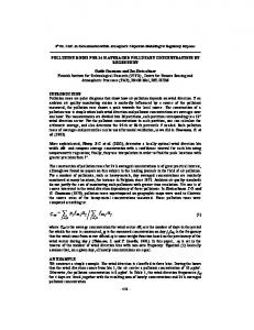
One quantitative method to demonstrate the safety compliance of a system is the evaluation of the system fault processing capabilities using fault injection. The general approach is to inject randomly selected faults into the system to determine if its fault processing capabilities mitigate the faults. The methodology is outlined in Figure 1.1 and consists of the following steps: 1. An analytical safety model is developed from the system architecture and inter-component dependencies to derive an expression for the selected safety metric. This expression is a function of critical model parameters such as the fault coverage values and failure rates for the various components of the system.
3
Numerical safety specification target and confidence level
Estimate of safety metric at required confidence
Step 1: Development of an analytical safety model Critical model parameters
Parameters estimates
Step 2: Development of a statistical model Number of experiments to perform Step 3: Development of a processor fault model
Step 4: Selection of the operational profiles
Step 5: Creation of the fault-free execution traces
Step 6: Fault list construction
Step 7: Analysis of the fault list using fault equivalence
Step 8: Fault injection experiment execution
Faults remaining in fault list?
Yes
No Remaining operational profile? Step 9: Analysis of fault injection experiment results
Yes
No
Figure 1.1: Safety evaluation process using fault injection
4
2. A statistical model is then developed based on those found in published literature and is used to estimate the critical model parameters that are required by the analytical safety model. This statistical model is also used to calculate the number of fault injection experiments required to meet the numerical safety target for a given confidence level. 3. A high-level processor fault model is defined to specify the types of faults (and their associated probabilities) that will be injected into the system under analysis. This fault model typically builds upon the characterization of low-level internal processor faults at the higher register-transfer level, in order to demonstrate that faults injected on the actual hardware are representative of the low-level processor faults of concern. 4. One or more operational profiles are then defined which will be used to drive the inputs to the system under analysis during the fault injection process. The operational profiles must be representative of the different system configurations and workloads that would be experienced in actual field operation. 5. A fault-free execution trace is created for each selected operational profile that will be used to generate the list of faults to inject into the system under analysis. This trace will also be used during the analysis of the fault injection experimental results. 6. Using the fault-free execution trace and the fault categories from the processor fault model, a fault list construction algorithm is applied to generate a list of possible faults that can be injected into the system under analysis, and which are likely to have an effect on the system. From this complete set of responsive faults, a fault list selection algorithm is then applied to randomly select a list of faults to be injected into the sys-
5
tem, using the fault categories and associated occurrence probabilities from the generic processor fault model. 7. A fault equivalence algorithm is applied to each fault list to identify those sub-sets of faults which will have the same effect on the system, known as fault equivalence classes. The set of faults to be injected into the system is then reduced using the fault equivalence information, since only one fault from each class needs to be injected. This reduces the amount of time required to perform the evaluation of the system under analysis by reducing the total number of fault injection experiments which must be performed. 8. Each fault from each reduced fault list is then injected into the system under analysis. The next section of this chapter will present several fault injection techniques that can be resorted to during this step. 9. The system is monitored during each fault injection experiment, and each fault is classified as covered, uncovered, or non-responsive by comparing the actual execution trace to the fault-free execution trace. Note that step 6 considerably reduces the number of non-responsive faults. Once all of the results of the fault injection experiments have been collected, they are fed back into the statistical model to calculate the estimates of the critical model parameters. The parameters estimates are then in turn fed back into the analytical model to calculate the selected safety metric, as shown in Figure 1.1.
6
1.2
Fault injection techniques
The safety evaluation method heavily relies on fault injection to characterize the response of the system under study in the presence of faults. Several fault injection techniques have been developed, each of them having its own advantages and shortcomings, and its own set of tools. Fault injection techniques can be divided into three main categories: hardware-based fault injection, software-based fault injection and simulation-based fault injection. The following subsections provide an overview of these three fault injection methodologies. Special attention will be devoted to simulation-based fault injection, since it directly relates to this research effort.
1.2.1
Hardware-based fault injection
Hardware-based fault injection involves additional equipment to introduce faults into the hardware of the system under study. Hardware-based fault injection techniques can be categorized between fault injection with contact and fault injection without contact [14].
As far as injection with contact is concerned, the injector is directly able to produce voltage and/or current variations at the pin level in the target system. It is in turn possible to distinguish two approaches: probes and sockets. Probes do not require the target chips to be disconnected from their support board, and are thus placed on the pins of the chips to force the value of the signals they carry. To the opposite, sockets are inserted between the chips and the support board. This technique limits the risk of damage since the signals are no longer forced. Fault injection with contact is limited to corrupting signals that are external to the chips and cannot corrupt, say, a register within a processor.
7
A hardware fault injector without contact has no physical connection to the hardware of the system under study. Faults are injected in the hardware through disturbances created by radiation or electromagnetic emissions. This technique allows fault injection in locations that are very hard to reach, for instance circuits that are located inside chips, yet does not provide a great amount of control on the exact locations where the faults appear.
A major benefit of hardware-based fault injection is that it preserves the actual software when running the experiments. Also, it operates in real time, and provides a very high resolution as far as the time of injection is concerned. The technique has its shortcomings too, the main criticism being the need of special purpose hardware. Also, the technique induces a potential risk of damage for the system under study, and the set of injection points can be limited due to the ever increasing integration of computer chips.
Numerous software fault injection tools have been developed over the years, including: Messaline [2], FIST (Fault Injection system for Study of Transient fault effects) [12], MARS (MAintainable Real-time System) [23], RIFLE [30]. These tools will not be described in details here, but additional references, such as [14], [33], and [42] list and review their main characteristics.
1.2.2
Software-based fault injection
Unlike hardware-based fault injection, software-based fault injection does not require any special hardware. A software-based fault injection technique is characterized by the modification of the program being run by the system under study. This technique can be used to
8
emulate hardware faults, but also software defects, or bugs. As far as hardware faults are concerned, only those locations that are accessible to machine instructions are potential candidates for faults.
Two principal approaches exist as far as software-based fault injection is concerned: compile-time fault injection, and runtime fault injection [14]. Those two differ regarding the time when faults are injected. The former method essentially aims at corrupting the code of the target program prior to its execution, hence creating an intrinsically erroneous piece of software. This method is attractive in a sense that, once the faults have been seeded in the code, no additional piece of software is needed during the execution of the program, which limits the perturbations on the target system. It is however difficult to adapt to faults to a particular workload, or operating profile. Thus, the controllability of this method is not optimal. With the latter method, runtime fault injection, faults are injected upon the occurrence of particular events. As an example, timeout triggered interrupts can be used to corrupt registers or memory locations.
The advantage of software-based fault injection is that it can be targeted to the application and operating system that are used on the system under analysis. Also, the experiments are fast, thus providing a good framework for large fault injection campaigns. Finally, there is no need for expensive additional hardware, and, since the software is running on the actual hardware, original design faults in the hardware are still present when running the experiments.
9
On the downside, this technique can only inject faults in those locations that are accessible to the software, that is to the machine instructions. Also, since the software code is modified, the experiments do not involve the exact same software package that is running on the system. The observability offered by the technique is limited, because, again, the scope of machine instructions itself is limited. A final point, the fault injection mechanisms can alter the scheduling and timing of system tasks, which can turn out to be a decisive drawback in systems where operations are time-constrained.
Numerous software fault injection tools have been developed over the years, including: GOOFI (Generic Object-Oriented Fault-Injection tool) [1], Xception [3], DOCTOR (integrateD sOftware fault injeCtiOn enviRonment) [13], FERRARI (Fault and ERRor Automatic Real-time Injector) [21], DEFINE (Distributed Fault Injection and Monitoring Environment) [22], FIAT (Fault Injection-based Automated Testing) [34]. Again, these tools will not be described in details here, but additional references, such as [14], [33], and [42] list and review their main characteristics.
1.2.3
Simulation-based fault injection
Simulation-based fault injection involves the construction of a simulation model of the system under analysis, including a detailed simulation model of the processor in use [42]. The system under analysis, often referred to as target, is thus simulated in another computer system, often referred to as host.
10
The advantages of simulation over the use of real systems are numerous. First, the simulation can be done at different level of abstraction, allowing for different fault models. Second, the injection of faults is not intrusive (a disadvantage of the software-based approach) because it happens immediately and transparently from the target system point of view. Third, among the three techniques, simulation-based fault injection offers the greatest amount of observability and controlability of both the target system and the fault injection mechanism. However, this approach has its limitations too. First, building a model of the target system usually consumes a lot of time and effort, and the results of the simulations are entirely dependant on how “good” the model is. Second, design faults in the actual systems may not appear in the simulation model. Finally, depending on the accuracy of the model, the fault injection experiments can rarely be done in real time.
A great amount of research work on simulated fault injection has been performed using the Very high-speed integrated circuit Hardware Description Language (VHDL). The principal VHDL fault injection techniques are listed in [11]. For example, the MEFISTO tool [18] resorts to the use of simulator commands, saboteur, and mutants. The simulator command technique is based on the use of the VHDL simulator commands to modify the values of the signals and/or variables of the models. This technique has the inconvenience of being simulator dependent. A saboteur is a special VHDL component that is added to the original model, while a mutant is an evolution of an actual component that encapsulates both its fault-free behavior and its faulty behavior. Both types of components have their shortcomings. The use of saboteurs hampers the simulation by adding a lot of complexity to the model. Mutants overcome this issue, but make it impossible to use the origi-
11
nal model without doctoring it. Other approaches, such as [7], use a technique known as bus resolution function, which basically allows two drivers to be connected to a unique signal, thus providing a basis for corrupting the value of the signal.
Like MEFISTO, VERIFY [35] is also a VHDL-based dependability assessment tool. VERIFY includes the reliability parameters into each behavioral component of the model. As such, the rate at which faults occur in each component, their durations, and their effects are part of the components descriptions. A positive point is that virtually any fault effect can be predefined. However, VERIFY uses extensions to VHDL, and thus require the development of a special compiler. Also, VERIFY illustrates the limitation associated with the use of mutants. Basically, the system model has to be entirely re-written to encapsulate the faulty behavior of each component.
REACT [4] is a software testbed that performs automated testing of multiprocessor architectures through the use of fault injection. Contrary to MEFISTO and VERIFY, REACT does not rely on VHDL, but instead uses the C language. REACT can model a variety of multiprocessor designs that utilize various redundancy approaches to implement fault tolerance. The target architectures are analyzed under the form of one, or several, processor(s), accessing memory modules through busses and error control logic blocks. Detailed models of processors architectures are not provided, and REACT only uses functionallevel abstraction of the processor(s) and memory modules.
12
DEPEND [10] is a simulation-based environment for system-level dependability analysis. It is a C++ functional simulation tool in which the target system behavior is described by a collection of processes that interact with one another. Those processes model the system behavior and the software. Actual programs can actually be executed in the simulation environment. The fault injection mechanism associates each component with a fault distribution. Several fault distributions are readily available, but the fault injector also allows user specified distributions. DEPEND provides a workload dependent injection facility to test systems under intense conditions.
Finally, the ADEPT tool [9], developed at the University of Virginia, is a system simulation tool for performance and dependability analysis. The tool is based on VHDL, and also encompasses a mathematical foundation provided by Colored Petri Nets (CPN) to support an analytical approach of the system under study. Dependability analysis can be performed in two different manners. First, the system level CPN model of the whole system can be automatically translated into a Markov model. This model can then be solved to yield the desired dependability metrics. The other approach relies on simulation based fault injection using the VHDL model of the whole system, and also uses the bus resolution function technique.
1.3
Simics overview
Simics is a platform for full computer system simulation, and provides a controlled, deterministic, and fully virtualized environment. Simics can be used to perform a variety of tasks, including support for the development of future commercial microprocessors, mul-
13
tiprocessor server memory architectures, high-performance fault-tolerant operating systems, testing of large networks, and hardware/software co-development.
The components of main interest in Simics are the processors. These are simulated at the instruction set level, and Simics currently is the first and most advanced commercially available, cycle accurate, instruction set architecture simulation tool. It supports a wide range of architectures such as: Alpha, AMD x86-64, PowerPC, UltraSPARC, or Intel x86. Simics also simulates all the hardware of a computer system, including controllers for memory, interrupts, PCI (Peripheral Component Interconnect), Ethernet, and so on.
These components work together with the processor chips to implement a fully functional virtual computer system, ranging from simple single-purpose embedded processors to complex full scale networks of high-end servers and clients. The concept of virtual system is illustrated by Figure 1.2.
The prototype system is the existing system that is being modeled, or the system that is being designed for example. The virtual system is made of the actual operating system and pieces of software, running on the virtual (that is, simulated) hardware. Finally, the host machine is running the Simics simulation tool that creates the virtual system.
As an example, consider Figure 1.3, which illustrates an x86/WinNT architecture simulated by a Simics session running on an x86/Linux host machine.
14
Web Server SPARC / SOLARIS
Prototype system
Virtual Web Server SPARC / SOLARIS
Virtual system
SIMICS HOST x86 PC / Linux
Host machine
Figure 1.2: Example of a Simics Virtual System A virtual computer system created by Simics is able to run unmodified operating systems, firmware, device drivers, middleware layers, network stacks, and application software. Although the chosen level of abstraction used to model the target system is low enough to run unmodified binary executables, it also mimics the interaction between software and hardware with a level of detail that does not hamper the performance of the simulation too much, which enables it to operate in realistic conditions by executing actual workloads.
A strong feature of Simics is its capability of providing a great amount of observability and controllability upon the simulated system. As such, the internal state of the processor, the content of memory, and the sequence of instructions that are being executed are visible at any moment. Furthermore, Simics comes with a proprietary API (Application Programming Interface) and encompasses some scripting features that can take advantage of this
15
Figure 1.3: A virtual computer running WinNT on a Linux host API to fully parameterize, control and automate the simulation. The API not only makes the state of the machine visible at any time, it also allows the content of registers or memory to be manipulated, which can be exploited to perform fault injection experiments. Finally, the simulation can be interrupted to take a snapshot of the complete system and save the current state of the simuation into a checkpoint file. The simulation can then be instantaneously resumed from this checkpoint.
Simics is built in a modular fashion. Its functionality can be augmented by developing custom extensions to satisfy specific needs (for instance, a tracing module that lists all
16
instructions being executed). Likewise, devices that are not included in the Simics default libraries (for instance, an analog acquisition card) can be developed and integrated into the configuration of a target system. Custom devices can be included in the simulation, mixed freely with the standard devices provided with Simics. Originally, Simics had not been designed as a dependability assessment tool, but owing to its flexibility, it is possible to include some fault injection capabilities, which will be detailed later.
As a complement, an exhaustive overview of Simics can be found in [31] and [40].
1.4
Contributions of this thesis
The goal of this thesis is to prove that Simics can be used as a dependability assessment tool for full computer systems by augmenting its possibilities with a fault injection module. This is a solid contribution to the scientific community because no other research work on simulation-based fault injection involves a commercial, cycle-accurate, instruction set architecture simulator that executes unmodified operating systems and application software.
DEPEND has been used for dependability analysis such as the one presented in [38]. The experiment involves a proprietary, cycle accurate, network simulator provided by Myricom Inc., and it is clearly stated that DEPEND is only used for software-level simulation, and does not execute the real code using the instruction set of the target system, but the instruction set of the host machine. REACT [4] provides a functional-level abstraction of the target system hardware, and is not able to use real code. VHDL-based techniques, like
17
the one proposed by DeLong et al. in [7], or the ones used in the MEFISTO tool [18], can intrinsically be used with cycle accurate VHDL models that are also able to execute machine instructions. However, to my knowledge, there is no such thing as a VHDL model of a complete computer system that is able to execute a full-blown software package with acceptable performance. The VERIFY [35] tool requires the development of a special compiler, and, finally, ADEPT [7] does not model the hardware/software interaction with a level of detail that allows the execution of actual software.
This thesis is organized as follows. Chapter II will introduce the fault injection technique based on Simics. Chapter III is devoted to incorporating a high level simulation of the physical environment of the target computer system within the Simics framework. Chapter IV is a detailed description of a proof-of-concept application which will serve to demonstrate the possibilities offered by Simics. A few fault injection experiments have been conducted on this application, using the newly developed fault injection technique, and Chapter V will present the results of those experiments.
18
Chapter 2 The saboteur module
2.1
Overview
In this research work, a specific Simics module, called saboteur module, has been developed to perform fault injection experiments as a support for the safety assessment methodology described earlier. This chapter presents a functional overview of the saboteur module, most of the implementation details being available in the source code included on the appendix CD. The saboteur module reads its inputs from a text file that contains the descriptions of all the faults that have to be injected during the fault injection campaign. As for now, a few commands have been implemented to control the new module. These commands also provide a means for automating the fault injection campaign via a simple script.
The next three sections describes the current level of development of the saboteur module. It is by no means definitive, as other types of faults and commands could be implemented to augment the functionality of the module.
19
2.1.1
Supported types of faults
The module is able to inject faults in several locations, either in a permanent or in a transient fashion. Faults can target a specific processor register, the data bus during a memory or I/O (Input/Output) operation, or the address bus during a memory operation. The way these corruptions are performed by the saboteur module will be detailed in later sections. The corruption of the address bus during an I/O operation is not fully supported yet, and reasons for this will also be explained later. In the case of a transient bus corruption, the saboteur module will corrupt the appropriate bus for the only operation that is being executed at the moment when the fault becomes active. In the case of a permanent bus corruption, the saboteur can either corrupt the appropriate bus for all the operations that are issued, or corrupt the appropriate bus for only those operations whose address match a user-specified address.
2.1.2
Description of the faults to inject
As said in the introduction, the saboteur module parses the fault descriptions from a text file which will be referred to as the fault file. We discuss here the various fields that are expected during this operation. Each line of the fault file describes a fault, and thus a fault injection experiment. Exactly 8 fields, separated by a tabulation character, have to be present: •
fault index: This field must contain an integer as a key to identify the current fault.
•
time of activation: This field must contain the number of seconds after which the current fault will be activated.
20
•
end of operation: This field must contain the number of seconds after which the current Simics session will be terminated. A new Simics session will be automatically launched, and the next fault in the fault list will be parsed.
•
target processor: This field must contain the name of the target processor, e.g. “cpu0”. This field is mandatory, since no default processor will be assumed.
•
fault class: This field must contain “transient” for transient faults, or “permanent” for permanent faults.
•
fault location: There are currently 4 supported fault locations. This field can only contain one of the following strings of characters: “register”, “memory
data
bus”, “memory address bus”, and “io data bus”. •
register name / address: For a register corruption, a register name is expected here, for example “eax”. For a transient bus corruption, this field actually is discarded. However, if the fault is permanent, the field can either be set to “n/a” or to an integer in hexadecimal form, for example “0xab12” (see “Supported types of faults” on page 19).
•
mask: The last field contains the mask that will be applied during the corruption. Each character of the mask targets a bit of the fault location, (for example the content of a register, or the address that is present on the address bus), the right most character of the mask being applied to the least significant bit. If the mask contains the character ‘1’ (respectively ‘0’), the corresponding bit will be set to 1 (respectively 0). If the mask contains any other character, the corresponding bit will remain unchanged. This mask representation has been retained because it allows to have a constant mask for stuck-at faults.
21
2.1.3
Commands
The saboteur module can be very easily controlled by three simple commands: source, inject and clear. These commands have been implemented to provide the basic functionality we can expect from such a module. •
saboteur0.source filename indicates to the saboteur module where the fault list can be found.
•
saboteur0.inject integer [filename] [-auto] indicates to the saboteur module which line of the fault list has to be parsed. An optional filename can be specified to log the activity of the module. Finally, if the “auto” flag is set, Simics will run in automatic mode. A section (see “Fault injection automation” on page 35) of this chapter is devoted to this aspect.
•
saboteur0.clear simply clears the current set up. In other words, the saboteur module becomes inoperative, the current fault is immediately deactivated, and all the objects that relate to the saboteur module are removed from the virtual machine.
2.2
Implementation
As an introductory note, let me first emphasize that, since the primary objective of this research was to assess the dependability of an Intel x86 based controller, the module has been tailored to this type of processor. The source code included on the appendix CD exhibits some particularities that result from this choice. Given that each Simics package focuses on a specific target processor, specific details inherent to processors that do not
22
belong to the x86 family have not been studied. Therefore, some implementation details might have to be changed to account for other types of processors/architectures.
2.2.1
Event posting
In essence, simulations running within Simics are driven by occurrences of events, such as instruction execution or device interrupt. The simulated processor (or each simulated processor in the case of a multi-processor configuration), is associated with a time queue and a step queue, both of which contain future events for the corresponding processor. In the step queue, the sequence of events is indexed on program counter steps, a step being either an instruction that has completed, or an instruction that has generated an exception, or finally an external interrupt. In the time queue, events are scheduled to occur with respect to time. However, given that the finest resolution offered for event posting is one clock cycle, the occurrences of events will be rounded down to the nearest clock cycle.
From a fault injection standpoint, the time queue is of particular interest, since faults are defined by the triplet {time, location, value}. As a matter of fact, the step queue has not been exploited in this research work, although it might turn out to be useful for some future extensions. The Simics API provides a few functions that allow the use of the time queue to post user-defined events, and this feature has been used in this research work to activate faults, perform some types of corruption (see “Processor register corruption” on page 23), and terminate the simulation.
23
As one can imagine, it is more than likely that several events are scheduled to take place during the same clock cycle. When this happens, the events are handled in the order they have been posted. However, the instruction execution event always occurs in last position. As a consequence, a user-posted event will always be triggered before the execution of the instruction that is scheduled at the same clock cycle. It is interesting to notice that, contrary to what has been done in some other simulation-based fault injection research projects, such as [7], no resolution function in necessary here, since neither registers nor memory will ever be assigned different values at the same time.
2.2.2
Processor register corruption
Using event posting, the corruption of processor register is fairly straightforward. The flow charts presented in Figure 2.1 and Figure 2.2 illustrate how this operation is performed, for both transient and permanent faults.
2.2.3
Memory busses corruption
Memory in Simics is represented by memory spaces [31]. This class of objects include physical memories and PCI (Peripheral Component Interconnect) bus spaces among others. The functionality of a memory space can be augmented by attaching some additional objects to it, provided that those implement some particular interfaces. A Simics interface essentially is a set of functions that are implemented by a Simics class, and that provide interaction between two objects, or between an object and the simulation core. More information can be found about interfaces in the Simics User Guide and the Simics Reference Manual. These particular interfaces are of two types: the timing model interface and the
24
START
post an event in the time queue that will activate the fault
wait until the fault becomes active
corrupt the target register
END
Figure 2.1: Flow chart for transient register corruption snoop memory interface. The following section discusses how an object implementing those two interfaces can interact with a memory space. 2.2.3.1
Memory spaces and interfaces
The timing model interface is used to return a number of idle cycles for a memory operation, and is thus typically used to create cache models, or to model the performance of a memory hierarchy. An object that implements this interface, also called a timing model object (or timing model), is called prior to every operation targeting the memory space to which it is connected. When called, a timing model receives a data structure describing the current memory operation, including the address that is accessed, the number of bytes that
25
START
post an event in the time queue that will activate the fault
wait until the fault becomes active
corrupt the target register
post an event in the time queue to wait one clock cycle
wait until the next clock cycle
has the register value changed?
yes
no
Figure 2.2: Flow chart for permanent register corruption are involved, and so forth. Then, the memory operation takes place. As an example, the trace module that is available with Simics implements this interface to build a trace of all the memory operations that are issued. A timing model not only has access to the characteristics of a memory operation, it can also alter them. More specifically, it can be used to
26
change the address of the memory operation (that is corrupt the address bus), and change the data that is written into the memory space (that is corrupt the data bus).
An object implementing the snoop memory interface, also referred to as a snoop device, interacts in a very similar fashion with the memory space to which it is connected, except that it is called after the completion of a memory operation. Naturally, the stall time specified by a snoop device is ignored since the operation has already been performed. However, it is still extremely useful because it allows to intercept the data that is read from a memory space. More importantly, it allows to change the data (i.e. corrupt the data bus) before passing the value to the processor.
The saboteur module implements both a timing model interface and a snoop memory interface, and can be connected to the main memory of a processor if the current fault has been identified as a bus corruption targeting the main memory.
The flow charts presented in Figure 2.3 and Figure 2.4 give a high level description of how these two types of interfaces can be used to perform both permanent and transient corruptions. 2.2.3.2
Cached memory operations
As a side note, a timing model is only called by a memory space when the current memory operation is not referenced in the Simulator Translation Cache (STC). The STC has essentially been designed to serve most memory operations directly, without systematically
27
START
3.1
post an event in the time queue that will activate the fault
load or store operation?
load
store wait until the fault becomes active
modify the data in the timing model
intercept the current memory operation
data or address corruption?
3.3
data
wait until the operation has completed
modify the data in the snoop device
3.3
address
3.2
3.2
modify the address in the timing model
3.3
3.1
3.3
deactivate the fault
END
Figure 2.3: Flow chart for transient memory bus corruption
28
START
4.1
post an event in the time queue that will activate the fault
intercept the current memory operation
wait until the fault becomes active
yes
target specific address? no
match current address?
yes
4.1
no
4.2
data or address corruption?
data
4.2
address wait for the next operation
3.1
3.2
3.1 and 3.2 then chain into 4.2 instead of 3.3
4.1
Figure 2.4: Flow chart for permanent memory bus corruption simulating the whole memory hierarchy of the target machine. Again, the Simics documentation provides some detailed information about the architecture of the STC. When the saboteur module is attached to a memory space, it is important to dump the content of the simulation caches so that all memory operations can potentially be intercepted and corrupted. To push the envelope further, when a memory operation is intercepted by the saboteur module (in other words, it has not been cached in the STC yet), we might want to
29
specify that future similar accesses will go through the memory hierarchy as well, especially for permanent faults. For transient faults, this is not a concern since the STC is flushed when the saboteur module is attached to its target memory space, that is at the same clock cycle when the fault becomes active, the current memory operation is intercepted and the corruption occurs. The code of the saboteur module shows how to implement these details. 2.2.3.3
Instruction fetches
By default, instruction fetches cannot be seen by a timing model or a snoop device. However, it is possible to activate this feature by changing the instruction profiling mode of the simulation. Again, the Simics documentation is more explicit about this topic. Naturally, enabling the profiling of instructions slows down the simulation, but it is necessary since instruction fetches are potential candidates for fault injection.
2.2.4
I/O busses corruption
Having in mind a high level overview of the x86 peripheral (I/O) subsystem is important because the fault injection techniques will differ depending on which element of the I/O subsystem the fault injection will target. The x86 architecture essentially comprises two classes of busses: the system bus, connecting the processor to the main memory and its associated cache, and a number of I/O busses, connecting various peripheral devices to the processor - the latter being connected to the system bus through a bridge (Figure 2.5).
30
Memory Processor
System bus
Bridge
Cache
I/O busses
Peripherals
Figure 2.5: General computer structure In addition to the memory address space, the x86 family of processors provides a 16-bit I/O address bus. However, I/O devices are not necessarily mapped on the I/O space, and can either be I/O mapped (the expression “port mapped” is a common synonym), memory mapped, or both. The 16-bit addressable I/O space actually became quite a limitation for some applications (for example, graphic cards), and memory mapped I/O devices easily overcome this problem since they look just like memory, and can take advantage of a much larger address space. For this type of I/O devices, the fault injection techniques that have been described in section 2.2.3 remain valid for both data and address corruption.
Different types of I/O busses have been introduced along the years. The most common are the ISA (Industry Standard Architecture) bus and the PCI (Peripheral Component Interconnect) bus. The more recent AGP (Accelerated Graphics Port) bus only deals with graphic cards, and is of little interest as far as fault injection is concerned. In addition, it is virtually inexistent in embedded systems. The other types of busses (VESA, EISA, and so
31
ISA devices ethernet card Processor
Port space
... keyboard timer
... Figure 2.6: A virtual processor and its port space forth) simply did not survive the test of time. The ISA bus was the first bus introduced in x86 based machines, its existence was gradually challenged by the arrival of newer busses, before being almost completely superseded by the PCI bus. It is still kept in place for slow devices and for compatibility with older systems. 2.2.4.1
Corruption of the data bus for PCI devices
The PCI bus is handled by Simics just like a regular memory space. As a result, the fault injection techniques that have been described to corrupt the data bus for memory operations can be applied for PCI devices. To this purpose, the saboteur module will connect itself to the PCI bus instead of the main memory. 2.2.4.2
Corruption of the data bus for ISA devices: a fundamental difference
As far as ISA devices are concerned, the corruption of the data bus during an I/O operation does not involve the same mechanisms. This comes from the fact that neither a timing model nor a snoop device can be attached to the object to which the ISA devices are connected. In the Simics environment, this object is know as the port space (Figure 2.6).
32
ISA devices
Processor
Port space
io-interface
ethernet card
...
...
io-interface
keyboard
...
timer
... Figure 2.7: Using the io-interface device
As seen earlier, the injection of a bus fault necessarily requires to intercept the operations that are issued by the simulated processor. Although Simics allows to place breakpoints on ‘in’ and ‘out’ instructions, which effectively intercepts port mapped I/O accesses, using breakpoints actually is excluded. Not only are breakpoint handlers triggered after an I/O access completes, but the access data structure is simply not available in a breakpoint handler. More generally, Simics provides no means for intercepting the I/O flow between the processor and its port-space.
To overcome that, a specific class of devices, dubbed io-interface, has been designed to monitor the I/O traffic on the port-space and to corrupt the data that passes to or from the processor. The code for the io-interface is available on the appendix CD. When needed, the io-interface device is connected to the port space, in place of the other devices (Figure 2.7). Those still remain in the configuration, and the io-interface will be in charge of accessing them upon request of the processor. In other words, the io-interface intercepts and forwards accesses from the processor to the ISA devices.
33
The io-interface device functions very much like the saboteur module does for the corruption of busses connecting the processor to a memory space object (Figure 2.3 and Figure 2.4). It does not act like a timing model or snoop memory per se, yet it corrupts the data either before calling the target device when the data flows back from the processor to the target device, or after the target device has completed the access when the data flows from the device to the processor. 2.2.4.3
On the limitations for corrupting the address bus during I/O operations
As said earlier, the corruption of the address bus during I/O operations is not fully supported. The structure of the peripheral subsystem for port mapped (as opposed to memory mapped) devices in Simics is the main cause of this restriction (Figure 2.8). Note that this figure does not necessarily reflect how I/O accesses would occur in a real system. Basically, any access that is not handled by the port space, in other words any access that targets a location where no device can be found, is forwarded to the PCI bus. The PCI bus is treated like a memory space, to the opposite of the port space. The reason for this is that their respective semantics are different. In a memory space, each address represents a single byte of data. In the ISA port space, each address can represent 1, 2 or 4 bytes of data. For example, if the processor reads, say, 2 bytes from the port space at a specified address, it can either receives 2 bytes from this address or 1 byte from this address and 1 byte from the consecutive address, depending on the device that is being called.
34
Processor
Port space
ISA devices
default PCI bus
PCI devices
Figure 2.8: Peripheral subsystem structure for port mapped I/O devices For a port mapped I/O access, it is not possible to corrupt the address before it hits the port space. The earliest moment when this becomes possible is either in the io-interface device if the access target an ISA type of device, or otherwise in a timing model attached to the PCI bus. Say, for example, that the latter case holds. If the timing model corrupts the address into an address that corresponds to one of the devices that are mapped on the port space, then the timing model has to cancel the access and forward it to the io-interface device. However, because of the difference of semantics between the PCI bus and the port space, it is in all generality impossible to do so.
For example, let us imagine that a timing model connected to the PCI bus receives a two byte read access at the address 0x400. Following a fault injection, imagine that the timing model has to corrupt this address into 0x300, which turns out to be the base address of a device that is mapped on the port space. As it is often the case, this device also occupies adjacent locations, such as 0x301 and 0x2FF. As stated above, the timing model has to forward the access to the io-interface. However, this could either be translated into a sin-
35
gle two byte access on the port space at address 0x300, or two one byte accesses at addresses 0x300 and 0x301. Thus, because of this ambiguity, corrupting the address bus for port mapped devices is not supported, and is left for future investigations.
2.2.5
Fault injection automation
A fault injection campaign consists in a sequence of simulation runs, each run corresponding to the injection of a single fault. Since a large number of faults have to be injected, the possibility of automating the injection process has been crucial in choosing Simics as a framework of this research.
The script run-simics (available on the appendix CD as well), launches Simics sessions in a sequential fashion. In other words, it creates a new Simics session as soon as it terminates the previous one. The scripts takes two file names as mandatory parameters, a checkpoint file and a fault list file. A third and optional file name can be specified to log the activity of the saboteur module. Before each run, run-simics updates an additional script, called saboteur.simics to parameterize the Simics session. The script basically tells Simics to load the saboteur module, indicates the appropriate fault list and indicates which fault to inject. Simics is then launched using both the specified checkpoint file and the script saboteur.simics.
36
Chapter 3 Full system simulation within Simics
3.1
Motivation
In reality, the actual controller from which the virtual controller has been derived is connected to a physical system to which it is providing command signals, and from which it is getting some information about the current state of the system. Therefore, simulating the controller itself is not very insightful from a fault injection standpoint, since it is difficult to derive the impact of the injected faults on the outside world. Accounting for the external environment of the controller, also referred as the plant, in the simulation framework not only allows to visually assess the impact of these faults, but it also allows to observe how the controller will in turn react when fed by signals produced by an incorrectly driven plant. Consequently, we ideally desire to have both the virtual controller and its plant simulated simultaneously, so as to directly observe how these two elements interact, hence the name of “full system simulation”. A computer system simulator, Simics has not been designed to simulate physical systems such as those usually driven by digital controllers. As a result, other simulation resources have to be conjugated with Simics in order to implement this concept.
37
3.2
Implementation
Different alternatives are available to use external simulation tools along with Simics. These are presented in [39]. Although this reference focuses on the use of an external simulator to provide detailed hardware models, typically at the signal level, instead of those included in Simics, the ideas it conveys still remain valid from a more general point of view. A first way to envision a dual simulation scheme is to interface Simics to an external simulator that takes care of the plant simulation (for example Simulink, the simulation tool edited by MathWorks), and have the two simulators work in parallel. This requires some sort of communication channel and communication protocol between the two tools, as explained in [39]. As an example, one could think of Simics as being the “master” simulator, commanding, say, Simulink, which would thus be configured as the “slave” simulator. The communication channel supporting the exchange of data between the two tools could be thought as shared memory structures which both simulators could access through wrapping layers that fit their semantics. This path has not truly been explored in the framework of this research, and is left for future investigations, as the other technique described beneath offers incontestable advantages.
A second approach, which is the one that we have retained and that has been implemented in this work, is to model the plant with an external simulator - as in the first approach, but then generate stand-alone C code from the plant model, and embed it in Simics. Since Simics devices are written in C, the resulting code can be easily wrapped into a custom device, which we will refer to as a wrapping device, and imported into any Simics simulation. The advantages of this approach are multifold. First, it involves a unique tool, that is
38
Simics, during the simulation per se, which considerably simplifies the simulation set-up. As a corollary, much to the contrary to the first approach, the development of a communication channel and a communication protocol is not required here. Second, all the features offered by Simics in terms of observability and controlability are immediately available. Hence, the wrapping device can be instrumented using the Simics API to provide any necessary information at any moment of the simulation. Furthermore, and this is a crucial point, when a checkpoint is created, the state of the external environment and all relevant information are stored along with the information that pertain to all the other devices in a unique file, which can then be reloaded to resume the simulation of the virtual controller and its plant.
3.2.1
Description of the wrapping device
3.2.1.1
Interaction with other devices
The plant driven by the actual controller takes as commands some voltage or current signals, typically delivered through digital-to-analog converters (DACs), and transmits information regarding its state to the controller via sensors and analog-to-digital converters (ADCs) and/or digital signals. Thus, in the simulation framework, the C code derived from the plant model must be provided with input variables that correspond to the various output channels of the virtual controller, and the outcome of its computation (that is the set of output variables), has to be fed to the input channels of the virtual controller. This is illustrated in Figure 3.1.
39
Actual system controller controller inputs
controller outputs
“plant”
Simics simulation framework
input devices
control application
input channels
Simics virtual controller
1-to-1 mapping
output variables
state variables
timing information
equivalent C code for the plant
output devices output channels 1-to-1 mapping
input variables
Wrapping device
modeling and C code generation
Figure 3.1: Integration of an external environment within the Simics framework
40
Naturally, the possibility of mapping input and output devices to an external environment must be accounted for when these devices are being built. Especially, one must be able to specify which environment wrapping device they are connected to, and which input - or output - variables of the device to which their channels are mapped. The code for the devices that have been developed to build a proof of concept application is available on the appendix CD, and exhibits how the mapping occurs, while the configuration script of the simulation, also listed on the appendix CD, shows how to interconnect the different devices to the environment wrapping device. 3.2.1.2
Calls to the device
The simulation of the external environment is not continuous, and does not take place in parallel with the simulation of the virtual controller. Much to the contrary, the simulation of the plant is triggered by the occurrence of events in the wrapping device. The environment wrapping device responds to two major sorts of events: either an output device (for example a) sets an input variable to a new value, or an input device (for example an. ADC) attempts to read the value of an output variable. Upon occurrence of such events, the wrapping device will have to simulate the behavior of the plant between the last event and the current time (that is the time of the current event) by running its embedded C code. At the end of each run, the state of the simulation has to be saved, as well as the current time, so as to be able to resume the simulation of the plant upon occurrence of the next event.
41
input device changes output variable ‘j’ t=0
t1
t3
t2
output device changes input variable ‘i’
time
output device changes input variable ‘i’
Figure 3.2: Occurrence of events in the wrapping device From a high level perspective, the wrapping device operates along the following sequence: •
retrieve the time of last event,
•
retrieve the last known state of the simulation,
•
run the simulation until the current time is reached,
•
update all output variables to reflect the new state of simulation,
•
update all state variables and the time of last event,
•
update input variables if required (first class of events).
The wrapping device contains appropriate storage - allocated during the compilation of the device code - to save the state of simulation and record the time of last event between two calls. The sequence above is quite intuitive, although it is important to note that the wrapping device has to run the simulation before updating any input variable, in case such an action is required by the current event. As an example, consider the three events shown in Figure 3.2.
42
Imagine that at time t=t1, a first event modifies the input variable ‘i’. A second event occurs at time t=t2, and also attempts to modify the same variable. The previous value of this variable (as set at t=t1) still prevails until the simulation of the plant reaches time t=t2. Therefore, the simulation first has to be advanced to the current time before accounting for any input variable modification, hence the step ordering described above. 3.2.1.3
Checkpointing
There are a few issues related to the checkpointing question that are worth discussing here. To put it briefly, the checkpointing operation consists in saving all the attributes of the device to a file. First, this implies that all the data that we wish to save during checkpointing be declared as attributes (see the device code on the appendix CD), which includes input variables, output variables, state variables and time of last event. Since output variables are accessed during this operation, the simulation will naturally be advanced to the current time before they are made available, and the time of last event will thus be the time at which the checkpoint was taken. Second, when the simulation is resumed from a checkpoint, all attributes are restored in the order they were declared in the device code. As a result, before input variables are restored to their last known values, it is important to first restore the time of last event, which in this case will match the current time, so that no simulation will take place. The reasons for setting such priorities are twofold. First, the simulation would have to start over from time 0 until the current time is reached, which might take a while if the model is complex and/or if the checkpoint was taken after a long time. Second, the simulation will likely provide incorrect outputs since it will only use the last known values of the input variables instead of accounting for all the variations that
43
they had been through during this period of time. If the precedence of time over input variables is respected, then output variables and state variables can be restored in any order with respect to the other attributes.
44
Chapter 4 Proof of concept application
4.1
Introduction and description
The original goal of this project was to develop a dependability assessment method relying on simulation based fault injection for the DFWCS (Digital Feed Water Control System) of the Calvert Cliffs nuclear power plant, located on the Chesapeake Bay. The DFWCS basically regulates the level of water in the steam generators of the plant. During the first months of 2002, we chose to use Simics as a platform for this work. The features offered by Simics, which have been exposed throughout the course of this document, were the driving force behind this choice.
In the course of the same year, it unfortunately turned out that it was impossible to complete the modeling phase for which I was required to build a model of the DFWCS hardware within Simics. The controllers that are used in this system are mainly made up of fairly standard PC parts, but the main obstacle that I encountered was a lack of architectural and behavioral details about the I/O (input/output) modules of the controllers. Those details are considered proprietary by the manufacturer and absolutely no information
45
regarding the implementation of these I/O modules was available. Since the key features of Simics is its ability to run unmodified software, the research group envisioned running the actual piece of software, that is an exact copy of the software running in the plant, on the virtual hardware emulated by Simics. As a result, developing our own I/O modules was ruled out in advance, since we did not even know how the software was accessing them.
As a result, it was decided that I should focus my efforts on developing a generic automatic fault injection process within the Simics framework. Once this step had been successfully completed, we still were unable to move forward with the DFWCS, and, as the goal of this research was, and still is, to prove that Simics could be used to perform fault injection in control type of applications, such an application had to be literally built from scratch.
4.1.1
An application inspired from the industrial world
The application that will be presented throughout this chapter is actually loosely based on a real application from the industrial world. We decided to adopt the main concepts on which the SpeedtronicTM Mark VI Gas Turbine Control system commercialized by GE is based. A introductory brochure is available at the following address: http://www.geindustrial.com/products/brochures/GEA-S1004.pdf. This micro-processor based control system is made up of three redundant control modules (Triple Modular Redundant - or TMR - architecture), each of them having its own power supply, processor, communication channels, and I/O to perform critical control of the gas
46
IONet link Controller 1
I/O board 1
IONet link
Controller 2
Controller 3
IONet link
I/O board 2
I/O board 3
IONet links : Communication board
Figure 4.1: Mark VI TMR architecture turbine. Most of the critical sensors are also triple redundant, to avoid single points of failures, although others - for example, monitoring sensors - are single element devices. The control functions of the Mark VI system include: acceleration, speed, load, temperature and fuel control. The turbine is also protected against abnormal conditions of the control and protection parameters.
The three controllers communicate between each other over IONet, an Ethernet-based network, and also access the triple redundant input/output boards using the same medium, resulting in three independent networks (Figure 4.1).
47
4.1.1.1
Input processing
An important part of the Mark VI fault-tolerant architecture also consists in reliably voting on the inputs and outputs of the control loops. The architecture shown in Figure 4.1 allows each controller to receive data from all the I/O modules. However, even if all inputs are available to all three controllers, several schemes exist to handle the data. For input signals that exist in only one I/O module, the same value is used by all three controllers. For signals that are available in the three I/O modules, their values may be voted upon to create a single, common value. The three signals can come from either replicated sensors, or from a single sensor whose signal is fanned out to the I/O boards.
Going through all possible {sensor redundancy, fanning, voting} combinations would be beyond the scope of this document. As an example, for speed inputs, signals delivered by redundant sensors are assigned as dedicated inputs to the I/O boards - each board is connected to its own sensor, and the values are then voted in software by middle value selection before being used by the controllers (see Figure 4.2). This technique is often referred to as Software Implemented Fault Tolerance (SIFT) [15]. 4.1.1.2
Output processing
The outputs delivered by the TMR system also go through some sort of fault-tolerant processing, but in a hardware fashion, as opposed to the software voting mechanism used for inputs. The three signals can either be voted upon by an external voting mechanism (for example, a voting relay driver), or they can be merged to produce a unique signal. This lat-
48
Sensors A
I/O board 1
Controller 1
B
I/O board 2
Controller 2
C
I/O board 3
Controller 3
: Communication board
mid-value selection
Figure 4.2: Software voting on dedicated inputs ter technique, know as flux summing, is particularly used for multiple-coils actuators. In the mechanism illustrated in Figure 4.3, the total magnetic flux created in the magnetic material is equal to the sum of the elementary fluxes created by each input coil. The output coil then produces a voltage that is a function of the total magnetic flux. Through the control loop, this mechanism automatically compensates for a spurious output delivered by a faulty controller.
4.1.2
Application description
The practical application that has been developed in the framework of this research is a fault-tolerant control system that regulates the speed of an electric motor. Although it is inspired from the SpeedtronicTM Mark VI system, a simplifying philosophy prevailed during its development, for a couple of reasons. First, conceiving a full-blown industrial application from square one would be an extremely time-consuming task, keeping in mind
49
Input coils
Output coil
ui1 uo
ui2 ui3
Magnetic material Figure 4.3: Flux summing mechanism that other objectives had to be fulfilled in parallel. Second, it was necessary to adapt the application to the Simics environment, hence the need for some modifications with respect to the original model. It is important to understand that building the proof of concept application has never been a goal in itself, but merely is a validation support for the fault injection technique presented earlier.
The system is based on a TMR architecture in which all three nodes are fully interconnected by an ethernet network (Figure 4.4). The speed sensors are triplicated, and, similarly to the configuration shown in Figure 4.2, the signals they deliver are assigned as dedicated inputs to the I/O ports of the controllers. Each controller is running under a commercially available Real-Time Operating System (RTOS), and implements a Proportional, Integral and Derivative (PID) control algorithm to regulate the speed of the motor. Soft-
50
Σ Controller 1
Controller 2
: Flux summing mechanism : Ethernet connection
Σ
+
Motor
Speed sensors
-
Controller 3
Figure 4.4: System architecture ware implemented fault tolerance is also used, and the output voltages delivered by the controllers go through a flux summing mechanism, which in turn feeds the electric motor.
There are a lot more details involved than this quick overview suggests.The next two sections (4.2 and 4.3) will deeply explain how the application has been implemented using the Simics framework. In the first section, we will examine how the virtual hardware has been developed. In the second section, the application software will be presented, focussing on the message passing and control algorithms, as well as the synchronization features.
51
4.2
Modeling and setting up the required hardware
The library of models offered by Simics has been the basis for putting together the three virtual controllers, whose core architecture is essentially made of basic PC parts, very much like one could expect to find in commercial off-the-shelf controllers. The virtual machines are based on an x86 Pentium type of processor, and include such elements as an ethernet card, 8 MB of memory, an IDE controller to handle a 40 MB hard drive (or as a support for flash memory cards), a VGA device for display, and other standard chips such as 8254 timer or a 8259 interrupt controller. Simics also offers network simulation, a particularly interesting feature in our case. However, a couple of other devices had to be developed to provide some analog I/O capabilities to the controllers. The concept of a wrapping device, presented in the previous chapter, was also developed to simulate the electric motor driven by the three controllers.
4.2.1
Network functionality
Fortunately, very little effort had to be made in order to establish a fully connected network between the three controllers of this application, given that the Simics library already includes an ethernet card. A particular Simics instance, called Simics Central, provides a virtual ethernet network to which multiple Simics sessions can connect via the ethernet-central module that Simics Central encompasses. The reader is invited to refer to the Simics documentation for a detailed description of the functionality of this module.
Simics Central handles the synchronization of the virtual time between all Simics instances that are connected to the virtual, simulated ethernet network. In other words, it
52
ensures that all Simics instances have the same time reference. This could turn out to quite problematic when, say, one Simics session simulates machines that are virtually sitting idle, while a second Simics session simulates heavy computational workloads. Since each Simics session basically runs as fast as it can, the time reference in the first session would pass at a much faster rate, drifting away from the time reference in the second session. As far as the application presented in this chapter is concerned, all machines are simulated within a unique Simics session, and thus already evolve in the same time reference.
4.2.2
Input/Output devices
The process of reading inputs delivered by speed sensors and producing voltage commands involves some sort of I/O devices that Simics unfortunately does not encompass in its standard library of components. As a consequence, it was necessary to develop such elements. To make it easier, simple analog-to-digital and digital-to-analog converters have been retained as a solution for providing I/O functionality. The code for the Simics devices that implement these two devices is available on the appendix CD. 4.2.2.1
Analog-to-Digital converter (ADC) device
An ADC basically converts an input voltage into a binary code for further digital processing. The Simics device that models an ADC is adapted from the MAX197 analog-to-digital converter. The documentation is available at the following address: http:// www.maxim-ic.com. The device simulates an 8 channel ADC that transforms its input voltage into a 12-bit word. In unipolar mode (Figure 4.5) the device will convert a positive voltage into an unsigned integer whereas, in bipolar mode (Figure 4.6), a positive or nega-
53
OUTPUT CODE
FS = ----------FS 1LSB = ------12 4096 2
11...111 11...110 11...101
00...011 00...010 00...001 00...000 0
1
2
FS -1 LSB
3
INPUT VOLTAGE (LSB) Figure 4.5: Unipolar Transfer Function tive voltage will be converted into a signed integer. The input voltage range of the ADC is known as the full scale (FS) voltage of the converter.
With reference to Figure 4.5 and Figure 4.6, the output code delivered by the ADC can be expressed as a function of the input voltage VIN: OUTPUT CODE =
CODE MAX – 1 ⁄ 2 1--- + V OUTPUT . IN -------------------------------------------------------------------FS – 3 ⁄ 2 × LSB 2
(4.1)
54
OUTPUT CODE
FS1LSB = 2-----------4096
011...111 011...110
000...001 000...000 111...111
100...010 100...001 100...000 0V
-FS
+FS -1 LSB
INPUT VOLTAGE (LSB) Figure 4.6: Bipolar Transfer Function In unipolar mode, the highest value of the output code, seen as an unsigned integer, is 3 n 2 – 1 , and is delivered for input voltages of FS – --- LSB and above. Furthermore, one 2 FS - , so that the output code is given by: LSB corresponds to an input range of -----n 2 n
OUTPUT CODE =
2 –3⁄2 1--- + V ------------------------------------IN n 2 LSB ( 2 – 3 ⁄ 2 )
=
V IN 1--- + ---------- . 2 LSB
(4.2)
55
In the bipolar mode of operation, the highest value of the output code is 2
n–1
– 1 and one
FS - . This actually leads, once simplified, to the same formula: LSB corresponds to ----------n–1 2 n–1
OUTPUT CODE =
2 –3⁄2 1--- + V -------------------------------------------IN n – 1 2 LSB ( 2 – 3 ⁄ 2)
=
V IN 1--- + ---------- . 2 LSB
(4.3)
The conversion is triggered when a control byte is written to the address at which the ADC is mapped inside the controller. The control byte also serves to select the full scale voltage (5V or 10V), the mode of operation (unipolar or bipolar), and the input channel. Other parameters can be defined in the actual MAX197, but since they were not required by the application, it is assumed that they are always set to 0, and only those modes that correspond to the 0 value have been implemented. I will mention those just for the sake of completeness. Only the internal acquisition mode has been implemented, which means that simply writing the control byte initiate the acquisition/conversion operation (ACQMOD is set to 0). Also, only the external clock mode has been implemented (PD0 and PD1 are set to 0 too). It is assumed that this external clock is constant and set at 2 MHz.
Finally, in the actual MAX197, the input channel voltage is stabilized after the acquisition period, which takes 6 cycles. Here, for the sake of simplicity, the input voltage is made available to conversion right away. To account for the acquisition and conversion time (respectively 6 cycles and 12 cycles), a 10 microseconds (approximately 18 clock cycles @ fCLK = 2MHz) delay is introduced before the new output code is computed. The device then flags the processor via an interrupt. Note that writing a new control byte during this amount of time simply starts a new acquisition/conversion cycle.
56
4.2.2.2
Digital-to-Analog converter (DAC) device
Conversely, a DAC converts a binary code into an output voltage to the outside world. The Simics device that implements the DAC is adapted from the Maxim MX7520 digital-toanalog converter, whose documentation is also available at http://www.maxim-ic.com Below are summarized digital-to-analog conversion relations for a 10-bit DAC. The tables presented here have been adapted from the documentation. Very much like the ADC, the DAC supports both unipolar and bipolar modes. In the unipolar mode, the relation between the output voltage and the input binary code is given by: DAC OUTPUT = DAC BIN × LSB .
(4.4)
LSB is the variation of voltage induced by flipping the least significant bit of the input binary code, and is given by LSB = 2
– 10
× V REF .
DIGITAL INPUT 1 1 1 1 1 1 1 1 1 1
ANALOG OUTPUT (1 – 2
– 10
) × V REF
1 0 0 0 0 0 0 0 0 1 1 – 10 --- + 2 × V 2 REF 1 0 0 0 0 0 0 0 0 0 V REF ⁄ 2 0 1 1 1 1 1 1 1 1 1 1 – 10 --- 2 × V 2 – REF 0 0 0 0 0 0 0 0 0 1
2
– 10
× V REF
0 0 0 0 0 0 0 0 0 0 0 Table 4.1: Code Table - Unipolar Binary Conversion
57
In the bipolar mode, the relation between the output voltage and the input binary code is given by: DAC OUTPUT = ( DAC BIN × LSB ) – V REF , with LSB = 2
DIGITAL INPUT 1 1 1 1 1 1 1 1 1 1 1 0 0 0 0 0 0 0 0 1
–9
× V REF .
(4.5)
ANALOG OUTPUT –9
( 1 – 2 ) × V REF 2
–9
× V REF
1 0 0 0 0 0 0 0 0 0 0 –9 0 1 1 1 1 1 1 1 1 1 – ( 2 × V REF ) 0 0 0 0 0 0 0 0 0 1
–9
– ( 1 – 2 ) × V REF
0 0 0 0 0 0 0 0 0 0 – V REF Table 4.2: Code Table - Bipolar Binary Conversion
4.2.3
External plant
As stated earlier, the three controllers are driving an electric motor. Specifically, a permanent magnet, direct current electric motor has been retained. An excellent description of this kind of device is available in [29]. The description and modeling section heavily relies on the material covered in this reference. We assume here that no load is attached to the rotor, which will simplify the electromechanical differential equations that describe the behavior of the motor even further. 4.2.3.1
Description and modeling of the external plant
Figure 4.7 represents the electric circuit of the kind of motor that is driven by the three controllers of the TMR system.
58
ra
Notations and dimensions: +
ia
i a is the current in the armature (A) r a is the resistance of the armature ( Ω )
La
L a is the self inductance of the armature (H) E a is the electromotive force (V)
ua
–1
k a is the back EMF constant ( V.s.rad )
+ Ea = ka ωr
–1
ω r is the angular speed of the rotor ( rad.s )
ωr
u a is the applied voltage (V)
-
2
J is the inertial moment of the rotor ( kg.m ) Figure 4.7: Schematic diagram of a permanent magnet, direct current electric machine Figure 4.7 has been adapted from [29], with the express consent of the editor, CRC Press. Considering this electric circuit and its corresponding notations, the Kirchoff’s voltage law yields: ka ra di a 1 = – ----- i a – ----- ω r + ----- u a . La La La dt
(4.6)
Also, the laws of Newtonian mechanics show that the angular acceleration obeys the following equation: d J ( ω r) = k a i a – B m ω r . dt
(4.7)
The term k a i a corresponds to the electromagnetic torque that is developed by the motor. The constant k a is the torque constant of the motor, expressed in N.m.A-1, and is equal to
59
ua + -
1 -----------------La s + ra
ia
ka
1 ------------------Js + B m
wr
ka
Figure 4.8: Equivalent s-domain block diagram for the electric motor the back EMF constant of the motor. The second term, B m ω r corresponds to the resistive viscous torque. It is proportional to the angular velocity, B m being the viscous friction coefficient expressed in N.m.s.rad-1. It naturally opposes itself to the torque produced by the motor, hence the negative sign. Again, it is assumed, for the sake of simplicity, that no load is attached to the shaft of the motor. If, however, it turned out to be the case, an additional resistive term should be included. The electromechanical coupling that takes place in the direct current machine can be described by the System 4.8 that combines Equations 4.6 and 4.7.
ra ka di a 1 = – ----- i a – ----- ω r + ----- u a La La La dt
(4.8)
Bm dω r k a = ----- i a – ------- ω r J J dt
This system of equations can be translated into the s-domain block diagram depicted in Figure 4.8.
60
As far as the order of magnitude of the parameters of the motor is concerned, there is a wide range of acceptable values, depending essentially on the manufacturer and the type of application. For instance, the Kollmorgen company, based in Radford, Virginia, carries the GOLDLINETM series of permanent magnet machines whose characteristics vary as presented in the table below.
Parameter
Typical range of acceptable values
La
from 1 mH to 300 mH
ra
a few ohms
ka
from 0.01 to 0.1 V.s.rad
J
from 1 × 10
–5
to 1 × 10
–3
kg.m
Bm
from 2 × 10
–6
to 2 × 10
–5
N.m.s.rad-1
–1 2
Table 4.3: Range of acceptable values for various motor parameters The choice for the values of those parameters is not of crucial importance for this proof of concept application. However, one has to keep in mind that the length of the time frame of the software application (recall, 40 milliseconds) has to allow for precise control of the motor speed. This implies that the time frame is short enough to capture the transient behavior of the motor, and the values of the parameters listed above have to be chosen accordingly. This matter is tackled in the Section 6.5 of [24]. The bottom line is that the time frame and the motor characteristics should be tied so as to “[obtain] 5 to 8 samples over the rise time of the process step response”. In order to satisfy this criterion, the following values have been retained: L a = 0.005 H, r a = 3 Ω , k a = 0.1 V.s.rad-1, J = 10
–3
2
–5
kg.m , B m = 10 N.m.s.rad-1.
61
600
500
angular velocity (rad/s)
400
300
200
100
0
0
0.5
1
1.5 time (sec)
2
2.5
3
Figure 4.9: Step response of the motor (input voltage = 50V) Using the s-domain diagram of the Figure 4.8, a simulation tool such as MATLAB can easily generate the step response of a motor having those characteristics (Figure 4.9). From this graph, the 90% rise time (i.e. the time at which the angular speed reaches 90% of its maximum value), is approximately 0.7 seconds. Thus, the criterion stated above is easily satisfied. 4.2.3.2
Simulation of the external plant
The previous chapter introduced a method for including an external system into the simulation framework, provided that this system can be fully described by a program using the C programming language. This naturally holds for this particular choice of plant. However, instead of resorting to a specific simulation tool such as Real-Time Workshop, a soft-
62
ware edited by MathWorks, it is relatively straightforward to directly develop some simulation code for this simple electric machine, and encompass it in a wrapping device. Numerical resolution of differential equations, a technique that is needed to write the simulation code, is presented in a great amount of details in [16], especially for equations of the form y' = f ( t, y ) . Among the different resolution methods that are available, the trapezoidal method offers both simplicity and relatively good accuracy for simple models. Over a small interval of time h, y’(t) can be approximated by: y(t + h) – y( t) y' ( t ) ≈ ----------------------------------- , h
(4.9)
and the trapezoidal method approximates f(t, y) by the average of its value at both extremities of the interval [t, t + h], that is: f ( t, y ( t ) ) + f ( t + h, y ( t + h ) ) f ( t, y ) ≈ -------------------------------------------------------------------- . 2
(4.10)
Thus, assuming that y0 = y(t0) is known at a given time t0, it is possible to recursively compute yn = y(tn) with t n = t 0 + n × h (for any positive integer n) using the formula: h y n + 1 = y n + --- [ f (t n,y ( t n )) + f (t n + 1,y ( t n + 1 )) ] . 2
(4.11)
Using Equation 4.11, the System 4.8 yields the System 4.12. h i = i a, n + --------- [ – r a i a, n – k a ω r, n + u a ( t n ) – r a i a, n + 1 – k a ω r, n + 1 + u a ( t n + 1 ) ] a, n + 1 2L a (4.12) h[ k a i a, n – B m ω r, n + k a i a, n + 1 – B m ω r, n + 1 ] ω r, n + 1 = ω r, n + ---2J hr a hk a hk a hB m Let us now introduce the parameters x 1 = ---------, x 2 = ---------, x 3 = --------, and x 4 = ----------. 2L a 2L a 2J 2J
63
The System 4.12 can in turn be transformed into a classic linear system (System 4.13) where only two variables, that is i a, n + 1 and ω r, n + 1 , are unknown. h i a, n + 1 ( 1 + x 1 ) + ω r, n + 1 × x 2 = i a, n ( 1 – x 1 ) – ω r, n × x 2 + --------- [ u a ( t n ) + u a ( t n + 1 ) ] 2L a – i a, n + 1 × x 3 + ω r, n + 1 ( 1 + x 4 ) = i a, n × x 3 + ω r, n ( 1 – x 4 ) (4.13) Both equations of this system can be combined into the matrix form: a c i a, n + 1 = e . f b d ω r, n + 1
(4.14)
The coefficients that allow for this transformation are: a = ( 1 + x1 ) , b = –x3 , c = x2 , d = ( 1 + x4 ) , h e = i a, n ( 1 – x 1 ) – ω r, n × x 2 + --------- [ u a ( t n ) + u a ( t n + 1 ) ] , f = i a, n × x 3 + ω r, n ( 1 – x 4 ) . 2L a Finally, the solution to this linear system of equations is given by: i a, n + 1 ω r, n + 1
1 = ------------------ d – c e , provided that ad-bc ≠ 0 . ad – bc – b a f
(4.15)
Note that ad-bc = ( 1 + x 1 ) ( 1 + x 4 ) + x 2 x 3 , which cannot equal 0, since all the xi coefficients are positive.
A wrapping device for Simics that performs the simulation of a permanent magnet, direct current electric machine has been developed, and its code is available on the appendix CD. The device implements the trapezoidal method described above, and relies on the motor
64
characteristics that were cited earlier. The simulation code also accounts for the flux summing mechanism, and takes care of scaling and adding the command voltages produced by the three controllers. Furthermore, it emulates the three sensors by assuming a linear conversion between the angular speed to the rotor and the and the resulting voltage, a relation that approximately holds in the case of magnetic speed pickups for example.
With reference to the previous chapter, the digital-to-analog device of each controller is mapped to a unique input variable in the wrapping device. As a result, three inputs are required. Similarly, the analog-to-digital devices are mapped to distinct output variables, to account for the fact that each controller has its dedicated sensor. As a final note, the fault injection module only targets location within the virtual controllers themselves, which excludes the variables produced by the wrapping device. For this reason, it would be equivalent, from a fault injection point of view, to map the ADCs to the same, unique, output variable.
4.3
Developing the appropriate software
The three controllers are executing µC/OS-II, a commercial Real-Time Operating Software (RTOS) developed by Jean J. Labrosse [25]. µC/OS-II is a preemptive real-time, multitasking kernel for microprocessors and microcontrollers. Preemptive means that the highest priority task that is ready to run automatically gains control of the processor, without having to wait for a lower priority task to relinquish the processor. Like µC/OS-II, most commercially available real-time kernels are preemptive. µC/OS-II was certified for use in an commercial avionics product by the Federal Aviation Administration, thus dem-
65
onstrating its robustness. µC/OS-II is used in commercial products by many companies, including American Power Conversion and Datacom among others.
In order to manage network connections, the key is to have a network programming library. Unfortunately, the feature is not present included in µC/OS-II. However, the University of Waterloo TCP (Transmission Control Protocol) library, WATTCP, is entirely free, although not supported by its original author Erick Engelke. It basically is a set of functions for creating and managing TCP/IP socket connections, and can effortlessly be linked to any µC/OS-II application. The library can de downloaded at http://www.wattcp.com. TCP is a widely used communication protocol, as opposed to proprietary or application specific protocols that obviously could not be used to build this application. TCP adds support to detect errors and loss of data, and to trigger retransmission until the data is correctly and completely received. To this extent, it is more reliable than other protocols such as UDP (User Datagram Protocol). The WATTCP library does not communicate with the ethernet card directly. Instead, it requires a packet driver. The packet driver is hardware dependant, and a whole list of various free drivers can be found at http:// www.crynwr.com/drivers/ for example. For the ISA ethernet card provided by Simics, the ne2100 packet driver, that is available at the address above, seems to work nicely.
4.3.1
Network setup and initial synchronization
The three controllers of the TMR architecture are connected together, thus forming a ring (Figure 4.10). Let us now have a closer look at how the ring is formed (Figure 4.11). Note that the WATTCP stack is not reentrant. In other words, the application software should
66
Controller 1
Ethernet network Controller 2
Controller 3
Figure 4.10: Connection ring not call the same function more than one time without waiting for it to return first. This implies that connections cannot be established simultaneously, but only one at a time. Similarly, the application software cannot send some data through two connections at the same time, and cannot read incoming data in parallel either.
That having been said, all controllers start by listening for an incoming connection, except controller 1 that attempts to open a connection with the next node in the ring counterclockwise, that is controller 2. Once the connection is established, controller 1 switches to listening mode, while controller 2 attempts to open a connection with controller 3. Once this step is over, controller 2 is connected to its two counterparts, and indicates that it has reached this state by sending a “ready” message to the two of them. It then waits for similar messages before starting the main application. At the same time, controller 3 attempts to open a connection with controller 1 in order to close the ring. When the connection is established, these two controllers send “ready” messages too.
67
initial synchronization lag
C1 C2 C3
t03 t01t02
C12
C23
C31
time
listening for incoming connection opening a connection sending ‘ready’ message to a distant node listening for incoming ‘ready’ messages from distant nodes acknowledging ‘ready’ message from a distant node t0i startup time of controller ‘i’ Cij connection between controller ‘i’ and controller ‘j’ is operational application software Figure 4.11: Creating the connection ring Each controller starts its application software only when it has acknowledged the fact that the other two nodes are ready as well (Figure 4.11). One could wonder how tight the initial synchronization provided by this very simple mechanism is. Figure 4.11 suggests that the synchronization lag is as short as the network latency. Knowing that the three controllers are forming a local, dedicated network, and are communicating using the TCP/IP protocol, it can be assumed that the maximum delay is not greater than a couple of milliseconds.
68
...
...
New frame begins
Allow background maintenance
Frame ends
Analog inputs/outputs manager Sending sensor value to a distant node Monitor incoming ethernet traffic, check for received messages SIFT + PID algorithm Figure 4.12: A typical frame of the application software The initial synchronization needs not be more stringent, given that the application software is based on a 40 milliseconds time frame.
4.3.2
Application software
After an initialization phase that basically starts the operating system, loads the TCP/IP support and establishes the peer-to-peer connections (see 4.3.1), the application software essentially consists in the repetition of a main frame at a regular interval T set to 40 milliseconds (Figure 4.12). This value is directly borrowed from the SpeedtronicTM Mark VI system.
Each frame begins with the application software reading the motor angular speed through the sensor connected to the controller, and delivering the voltage command that was computed during the previous frame (see “I/O devices manager” on page 69). Note that when the frame is executed for the first time, a null voltage is delivered. Once the speed of the
69
motor is available, it is sent to the other nodes of the TMR architecture over the network. Following this, the controller waits a certain amount of time (10 ms) for its counterparts to send their own values. It then performs a middle value selection on three values it has at its disposal, assuming the default value of 0 in case it has not received anything. Using the PID control algorithm, the new voltage command - that will only be delivered at the beginning of the next frame - is computed. The main frame then relinquishes the processor for a few milliseconds to allow the RTOS to perform some background work and maintenance. Finally the main frame is resumed, and the controller continuously checks for the possible arrivals of new messages until the end of the frame, the reason for this being that the synchronization lag between controllers might lead one of them to enter a new frame, and thus send its sensor value, while the others have not completed theirs yet. One could object that such an “early” message will be read in the next frame anyway. It is however important to record the time of reception of incoming messages by acknowledging them as soon as they arrive for resynchronization purpose, as explained in the section “Resynchronization algorithm” on page 78. Thus, the frame should be ended by monitoring the ethernet connections for a few milliseconds, at least.
4.3.3
I/O devices manager
The creator of µC/OS-II, Jean J. Labrosse, also provides a set of ready to use modules written in C for µC/OS-II [26]. One of theses modules provides the code for a task that manages analog inputs and analog outputs. This module has been used ‘as if’ in the application, the only custom code needed being the functions that handle the accesses to the analog-to-digital and digital-to-analog converters.
70
As far as the analog-to-digital device of the controller is concerned (see the corresponding section page 52), the control byte that selects the mode of operation and the input channel has to be written to the base address of the ADC. The device then flags the processor with an interrupt when the conversion is complete. As a result, an ISR (Interrupt Service Routine) has to be written to handle the interrupt. The file adc_isr.asm included on the appendix CD contains the assembly code. The ISR simply signals the end of the conversion with a semaphore, that essentially is a kernel object, managed by µC/OS-II, that accesses shared resources. Specifically, after writing the control byte, the function that attempts to read the ADC is pending on the semaphore that the ISR is supposed to post. When the semaphore is obtained, it means that the analog input has been converted, and the result is available to the application software.
Regarding the digital-to-analog converter, it is just sufficient to write the binary word to convert to the base address of the DAC.
The file cfg.c, available on the appendix CD, contains the functions that perform the access to the Simics ADC and DAC devices.
4.3.4
PID control algorithm
As an introductory note, let me first point out that this section intensely relies on the material presented in [24]. The reader is naturally invited to consult this reference for more ample details. On each three controllers, the application software encompasses a digital PID control algorithm. A PID control structure essentially comprises 3 components,
71
which are the Proportional, Integral and Derivative parts. Thus, the command signal delivered by a PID controller can be put under the general form: d 1 u = K c e + ----- ∫ e ( t ) dt + T d e = u p + u i + u d . dt Ti
(4.16)
The variable e designates the error between the desired value and the actual value of the controlled process. For a digital PID controller, this continuous-time expression must be re-written differently, to account for the fact that the controller now deals with discrete signals, obtained using a sampling period of T seconds. For the proportional part, we can simply write: u p ( kT ) = K c × e ( kT ) .
(4.17)
However, it is necessary to approximate the integral and derivative parts between two consecutive samples. Using a first order approximation, the integral of e(t) can be evaluated using the formula: kT
∫0
k
e ( t ) dt ≈
∑ Te ( kT ) ,
(4.18)
n=1
which is illustrated in Figure 4.13. As a result, we can approximate the integral part of the command signal with the recursive relationship: Kc u i ( kT ) = u i ( ( k – 1 )T ) + ------ × Te ( kT ) . Ti
(4.19)
Finally, the derivative of e(t) at time t = kT can be approximated by: e ( kT ) – e ( ( k – 1 )T ) d e ( t ) ≈ ------------------------------------------------- , dt t = kT T
(4.20)
72
k–1
e(t)
area =
∑ Te ( nT ) n–1
kT
∫0
(k-1)T
k–1
e ( t ) dt ≈ Te ( kT ) +
∑ Te ( nT ) n=1
kT
time
Figure 4.13: First order approximation of an integral so that the derivative part of the command signal can be computed as being: e ( kT ) – e ( ( k – 1 )T ) u d ( kT ) = K c T d ------------------------------------------------- . T
(4.21)
The z-transform notation is particularly well suited to describe the transfer function of discrete processes. For a digital PID controller, considering the approximations listed above, and introducing K i = T ⁄ T i , and K d = T d ⁄ T , the transfer function between e and u can be written as: z z–1 H ( z ) = K c 1 + K i ----------- + K d ----------- . z–1 z
(4.22)
As a reminder, given a signal x(t), if x(z) is the z-transform of the sequence xk, with xk = –1
x(kT) and m ≤ k ≤ n , then z x ( z ) is the z-transform of the sequence x k – 1 . It is then relatively straightforward to derive the expression of H(z) from the expressions of u p ( kT ) ,
73
Digital PID control
command +
-
e(t)
e(kT) kT
z ---------z–1
T ----Ti
z---------– 1z
Td -----T
electric motor
+
Kc
u(kT)
Figure 4.14: Z-domain block diagram of a digital PID control process u i ( kT ) and u d ( kT ) . Very much like we presented a s-domain block diagram of the electric motor earlier, we can also represent H(z) with a z-domain block diagram, as illustrated in Figure 4.14.
Since the electric motor will be driven by three controllers instead of one, the application that is described in this chapter does not exactly correspond to what is depicted in Figure 4.14. However, it is quite a convenient representation to envision those three machines as whole unity for now. Each controller will indeed run its PID algorithm just as if it was on its own. The output voltages will naturally have to be scaled down, to provide a voltage tantamount to the one delivered by a simplex configuration, i.e. an application comprising a unique controller, in the fault free case.
74
Tuning the PID controller, or any type of controller for that matter, is naturally a key step in building a control application. It can also turn out to be quite tricky as the three parameters, Kc, Ti and Td have opposed effects [24]. Typically, increasing Kc will increase the rapidity of the response of the controlled process, but will decrease its stability, while increasing Ti will have to opposite effect by removing the steady-state error and decreasing the rapidity of the process. On the other hand, Td can be used to increase to stability, and the speed as well, but will not do much for correcting the steady-state error.
In the 1940’s, Ziegler and Nichols [43] proposed two relatively straightforward methods for tuning PID controllers. The first one is based on the open loop step response of the uncontrolled process, while the second one is based on the process connected to a simple proportional control. The latter has given excellent results for tuning a digital PID controller to drive the electric motor that has been described earlier.
Kiong et al. in [24] describe this method as follows: •
With the integral and derivative parts turned off, increase the gain until the stability limit is reached (self oscillation). Let Ku and Tu be the gain and the oscillation period.
•
Once Ku and Tu are know, the Ziegler-Nichols frequency response recommends the following settings: Kc = 0.4 Ku, Ti = 0.5 Tu, Td = 0.125 Tu.
Using the diagrams shown in Figure 4.8 and Figure 4.14, it is very easy to apply this method with a tool such as MATLAB/Simulink. The first step is to reach the stability limit
75
600
500
angular velocity (rad/s)
400
300
200
100
0
-100
0
0.2
0.4
0.6
0.8
1 time (sec)
1.2
1.4
1.6
1.8
2
Figure 4.15: Response obtained with a simple proportional control (K = 0.79) with a simple proportional control by progressively increasing its gain. After a few trials, the limit apparently sits around K = 0.8, as illustrated in Figure 4.15 and Figure 4.16. Both were obtained with a command signal of 300 rad/s.
Looking at Figure 4.16, for Ku = 0.80, about 17.5 oscillations are recorded over a 4 seconds interval, hence the oscillation period Tu can be set to 228 ms. Then, according to the Ziegler-Nichols, a good set of parameters for the PID control structure should be: K c = 0.32 , T i = 114 ms and T d = 28.6 ms
76
600
500
angular velocity (rad/s)
400
300
200
100
0
-100
0
0.2
0.4
0.6
0.8
1 time (sec)
1.2
1.4
1.6
1.8
2
Figure 4.16: Response obtained with a simple proportional control (K = 0.80) The Ziegler-Nichols does not provide an ‘ideal’ solution by any means. It is more intended to provide a basis for fine tuning. As one can see by looking at Figure 4.17, the motor effectively settles on the command value (300 rad/s), but the overshoot phenomenon is quite present, and it is necessary to tweak the parameters to achieve a better result. By changing the values a little bit, it turns out that the derivative part does not contribute to improve to control of the motor that much, and a simple PI controller actually provides quite a good result, when tuning Kc around 0.3 and Ti around 0.2 sec. (Figure 4.18).
No real optimization effort has been carried out as far as tuning the PID structure is concerned. Refining the PID control algorithm was certainly not a top priority with respect to the original goal of this research work and the tuning problem is just one aspect of the
77
600
500
angular velocity (rad/s)
400
300
200
100
0
0
0.2
0.4
0.6
0.8
1 time (sec)
1.2
1.4
1.6
1.8
2
Figure 4.17: Result obtained when tuning the digital PID with the Ziegler-Nichols method
600
500
angular velocity (rad/s)
400
300
200
100
0
0
0.2
0.4
0.6
0.8
1 time (sec)
1.2
1.4
1.6
Figure 4.18: Result obtained with a better tuned PID
1.8
2
78
application, among many others. It was however absolutely necessary to come up with a good control algorithm, so that the application behaves correctly and provides some relevant information and data.
4.3.5
Resynchronization algorithm
The final section of this chapter deals with keeping the three controllers of the TMR architecture synchronized within the initial synchronization bound, that is a couple of milliseconds. The problem here is to ensure that the three controllers keep on executing their respective software frames in synch, knowing that they are approximately synchronized when the application software starts. Each controller times its actions with respect to its own clock. For example, each frame is timed to last 40 milliseconds, and the RTOS is in charge of enforcing this requirement. However, no clock keeps perfect time, all drift with respect with some reference standard time [32]. Of course, in a simulation tool like Simics, this issue does not transpire, thanks to the complete determinism of the simulation. Nevertheless, in a real system, there is obviously no reason for the clocks in the TMR system not to drift away from one an other, and the software has to take this into account. This indeed leads to the software frames lasting a little more, or a little less, than the “ideal” 40 ms, so that the three computers might ultimately be completely out of synchronization if nothing is done to adjust their lengths from time to time.
As Jalote explains in [17], an attempt to synchronize clocks will somehow require the processors to get the value of other clocks. Since the exchange of clock values will occur over the ethernet network, a first obstacle in establishing clock synchronization is to account
79
for the - non constant - communication delay. The second obstacle is that clocks can be faulty too. It has been shown in [8] that it is impossible, in a triple modular system, to achieve synchronization in the presence of malicious faults. A typical example of malicious faults, also known as Byzantine, is dual faced clocks: controller 1 sending the value 2:00 to controller 2 and the value 3:00 to controller 3 is a common scenario cited in the literature. If unforgeable digital signatures are available, and they are not in this application, then synchronization can be achieved with only three nodes, but in all generality, four nodes are required to handle one malicious fault (or 3m+1 nodes to tolerate m faults). The algorithms presented by Lamport and Melliar-Smith in [27], including the widely-used interactive convergence algorithm, fall in both categories.
The algorithm that is used in this application is adapted from the algorithm presented by Lundelius and Lynch [28]. This algorithm was originally designed to handle all kind of faults, including malicious faults, but can equally be used in a TMR architecture if it is assumed that clocks are not subject to Byzantine types of faults. The algorithm can easily be incorporated in the frame structure. To achieve synchronization, the length of the frames are adjusted by modifying the length of the last phase (noted “A” on Figure 4.19).
When the application software begins, the local time is resetted to 0. At this point, as explained earlier, the controllers are synchronized within the upper bound of the network latency, typically a couple of milliseconds on a dedicated local network. In each frame, after sending the messages over the network, the current time T is recorded. We assume that no resynchronization occurs in the very first frame. For all subsequent frames, when
80
Record current time T
...
Tadj
B
Ts: new frame begins
background maintenance
A
...
TA
Te: frame ends
Analog inputs/outputs manager Sending sensor value to a distant node Monitor incoming ethernet traffic, check for received messages, and collect arrival times of messages SIFT + PID algorithm Figure 4.19: Adding synchronization to the application software the software reaches Tadj, it substracts the middle value of the arrival times collected during A and B, including T, to T itself. Note that the arrival times of messages that were received during A are smaller than T because they were collected during the previous frame, while the arrival times of messages that were received during B are greater than T. This yields a corrective variable ∆T that is used to adjust the length of A, TA, for the current frame. TA is obtained by the following formula: T A = 40 – ( T adj – T s ) – ∆T ,
(4.23)
where all variables are expressed in milliseconds and Ts designates the time marking the beginning of the current frame. As a final note, the inputs/outputs manager does not take more than 20 µs to execute (see “I/O devices manager” on page 69), and therefore does not mask the arrival of messages for a significant amount of time.
81
Chapter 5 Experiments
In order to demonstrate the capabilities of the fault injection module that has been developed in the Simics environment, a few faults have been injected using this module while Simics was being used to run the control application described in the previous chapter. The impact of the injected faults can basically be observed by monitoring the evolution of the angular velocity of the motor over time, and comparing this curve to the same curve obtained in fault-free conditions. The next sections of this chapter will detail these fault injection experiments and exhibit the results that were obtained. The experiments were performed using Simics version 1.6.9, that was released in July 2003. The host system is a dual Pentium III system, in which each processor is running at 700 MHz. The operating system is RedHat Linux version 9.0. All configuration files are included on the appendix CD.
5.1
Instrumenting the target system
Any Simics device is characterized by attributes, which basically enable other devices to set, or get, the internal variables of the device structure. In particular, the concept of
82
attributes can be exploited to monitor the system under study. As such, when a fault is injected in the virtual system and becomes active, a predefined function is called by the saboteur module. The body of this function can be defined by the user to perform any action required to obtain information about the current state of the system. As a example, the reader is invited to refer to the function monitor_start_hook(), that can be found in the file monitor.c on the appendix CD. Note that this example is specific to the application described in this document. The saboteur module calls this function when it activates the current fault. This function in turn calls the auxiliary, user-defined function, read_speed_handler() that reads the actual angular velocity of the motor through the appropriate attribute of the wrapping device that encapsulates the code that simulates the electric motor. The value is written into a file along with the current time stamp, and the function schedules itself every five milliseconds using the event posting feature of Simics.
5.2
Fault-free output
In order to capture the fault-free behavior of the motor, the saboteur module also accepts a special class of faults that are idle faults. These are not faults per se: when such a “fault” is activated, the saboteur module actually does not do anything, but simply calls the monitoring hook function described above. As a result, the system under study in running in faultfree conditions. A preliminary simulation run indicates that the control loop of the application software begins slightly after the simulation time reaches 4 seconds. This corresponds to the amount of time required for the three controllers to boot, initialize their operating systems and establish the ethernet connections. After bringing the simulation to this point,
83
600
500
anuglar velocity (rad/s)
400
300
200
100
0
4
4.2
4.4
4.6
4.8
5 time (sec)
5.2
5.4
5.6
5.8
6
Figure 5.1: Fault free output the angular velocity of the motor can be logged by loading the saboteur module and supplying the following parameters: fault index: time of activation: end of operation: target processor: fault class:
1 0.0 2.0 ctr1_cpu0 idle
The evolution of the angular velocity of the motor over time can then be plotted from the file generated by the saboteur module. The result is given in Figure 5.1. Note that this figure is very close to Figure 4.18, that was obtained from a high level MATLAB/Simulink model of the system {motor + digital PID}, based on s-domain and z-domain block diagrams of these two elements. The slight discrepancy between the two figures can be
84
Figure 5.2: TMR applications running explained by the fact that the trapezoidal method used to model the electric motor in the wrapping device is not as precise as the method used by MATLAB/Simulink (see section 4.2.3.2 “Simulation of the external plant” on page 61). As far as the performance of Simics is concerned, it varies largely, depending on the workload that the virtual machines are going through. Typically, when the application software is running, each software frame is simulated in about 3 seconds, hence a 75 slowdown factor.
Figure 5.2 is a screenshot of the three applications running in parallel on the virtual controllers created by Simics.
85
5.3
Fault injection experiments and results
The third step of the numerical safety evaluation process (see section 1.1 “The numerical safety evaluation process” on page 2) stresses the need for a processor fault model. The processor fault model is used to build the fault space, a multi-dimensional space than can encapsulates fault characteristics such as location, time and value. Numerous efforts have been carried out in this field along the years, including research work performed at UVa such as [6], that in turn borrows from other publications such as [41]. The current state of development of the saboteur module actually largely supports the processor fault model presented in [6], exception made of the corruption of the address bus during I/O operations (see section 2.2.4.3 “On the limitations for corrupting the address bus during I/O operations” on page 33). Again, the reader has to keep in mind that this thesis aims at demonstrating that Simics can be used as a fault injection tool. As such the saboteur module is not geared to any particular processor fault model, and, naturally, could be modify to accommodate other types of faults.
5.3.1
Operational profiles and traces
With reference to Figure 5.1 the angular velocity of the motor first goes through a transition phase, before stabilizing to the desired value. As such, two primary operational profiles can be distinguished. For each of these profiles, a trace, that is a sequence of all the instructions and memory operations that are executed in the system, of a few milliseconds was created. These two traces were generated with the tracing module included in Simics, although this module had to be enhanced to display the current time of the simulation as well.
86
A typical trace can look like the following lines: [5.038146450000] inst: [ 554] CPU fe 4e ec data: [
383] CPU
Vani WB Read data: [
1 bytes 384] CPU
Vani WB Write
1 bytes
0
dec byte ptr [bp]+0xec 0 0x4f 0 0x4e
[5.038146500000] inst: [ 555] CPU 75 33
0
jne 0x1db9
For example, the first line indicates that an instruction has been fetched from the memory at time 5.03814645. This is followed by the processor that issued the operation, the current code segment, the linear address and the physical address of the operation, and the opcode and its associated instruction. The traces were used to determine when and where it was pertinent to inject some faults. For instance, considering the trace listed above, one could choose to corrupt the data bus at time 5.03814645 so that the corresponding processor would obtain an incorrect opcode.
5.3.2
Injected faults
The first “fault” that was injected into the TMR application actually is the idle fault that we discussed earlier, which was necessary to determine the fault-free output of the system. Ten other faults were also injected to demonstrate the capabilities of the fault injection modules. Note that all faults were injected into the same controller. Their characteristics, and the outcome of the injections, are summarized in the following subsections.
87
5.3.2.1
Fault 2
Fault 2 is a fault targeting the I/O bus while the application attempts to obtain the angular velocity of the motor. The precise time of injection was derived from the traces created beforehand. The fault parameters are as follows: fault index: time of activation: end of operation: target processor: fault class: location: address: mask:
2 5.03811865 7.0 ctr1_cpu0 transient io data bus (not needed for transients) 0000000000000000 (0x0)
This fault actually had no impact on the output of the system. This comes from the fact that the signals delivered by the sensors are voted in software being processed by the controllers. The angular velocity of the motor follows the curve of Figure 5.1. 5.3.2.2
Fault 3
Fault 3 is a permanent corruption of the I/O bus at address 0x75, that is the address at which the digital-to-analog converter is mapped (see the configuration files on the appendix CD). This fault forces this device to deliver the maximum voltage constantly, and thus emulates a permanent failure of the DAC. The fault parameters are as follows: fault index: time of activation: end of operation: target processor: fault class: location: address: mask:
3 5.0 7.0 ctr1_cpu0 permanent io data bus 0x75 1111111111111111 (0xFFFF)
88
600
500
anuglar velocity (rad/s)
400
300
200
100
0
4
4.5
5
5.5 time (sec)
6
6.5
7
Figure 5.3: Output of the system when submitted to fault 3 The impact of the fault is illustrated by Figure 5.3. The two non-faulty controllers are able to mitigate the faulty DAC, hence demonstrating the fault-tolerant properties of the flux summing mechanism. However, the output takes about a whole second to settle back to the setpoint value. 5.3.2.3
Fault 4
Fault 4 is a transient corruption of register eax. The time of injection was selected so that the register contains the value that will be sent to the DAC. Again, this was made possible by the use of the system traces established earlier.
89
600
500
anuglar velocity (rad/s)
400
300
200
100
0
4
4.5
5
5.5 time (sec)
6
6.5
7
Figure 5.4: Output of the system when submitted to fault 4 The fault parameters are as follows: fault index: time of activation: end of operation: target processor: fault class: location: register: mask:
4 5.0381288 7.0 ctr1_cpu0 transient register eax xx010x110x1x0x01
Figure 5.4 clearly illustrate the impact of the injected fault on the angular velocity of the motor. Note that the hardware redundancy is not responsible for correcting the faulty output here.
90
5.3.2.4
Fault 5
Fault 5 is a transient corruption of the data bus during an instruction fetch. The objective was to have the target processor execute an incorrect instruction. However, no effect could be detected, neither on the output of system, nor on the behavior of the controller itself. The fault parameters are as follows: fault index: time of activation: end of operation: target processor: fault class: location: address: mask:
5.3.2.5
5 5.03830925 7.0 ctr1_cpu0 transient memory data bus (not needed for transients) 1x001x11
Fault 6
Fault 6 is a permanent corruption of register ebx during the stabilized phase. The fault parameters are as follows: fault index: time of activation: end of operation: target processor: fault class: location: register: mask:
6 5.0 7.0 ctr1_cpu0 permanent register ebx xxxxxxxx10101010 (lower byte set to 0xAA)
Although the target controller freezes (as illustrated by Figure 5.5), the motor still sustains the desired speed. This stems from the fact that the DAC of the faulty controller keeps on
91
Figure 5.5: Impact of fault 6 on controller 1 delivering the correct voltage. However, if the setpoint was to change, or if the fault had been injected during a transition phase, then the performance of the system would have been altered. This will be illustrated by fault 10. 5.3.2.6
Fault 7
Fault 7 is a permanent corruption of the data bus when memory location 0x30cd5 is accessed. The fault parameters are as follows: fault index: time of activation: end of operation: target processor: fault class: location: address: mask:
7 5.0 7.0 ctr1_cpu0 permanent memory data bus 0x30cd5 00xxxx1110101111
92
Figure 5.6: Impact of fault 7 on controller 1 The only noticeable effect of this fault was a corruption of the display, as illustrated by Figure 5.6. 5.3.2.7
Fault 8
Fault 8 is a permanent corruption of the data bus for every memory operation. The fault parameters are as follows: fault index: time of activation: end of operation: target processor: fault class: location: address: mask:
8 5.0 7.0 ctr1_cpu0 permanent memory data bus n/a 00001111 (0x0F)
93
As one could expect, this causes the target controller to freeze. Injecting this type of fault is computationaly intense, as suggested by the 40 minutes simulation time. This slowdown is due to the fact that the saboteur module is intercepting all memory operations, and is not allowing them to be cached (see section 2.2.3.1 “Memory spaces and interfaces” on page 24 and section 2.2.3.2 “Cached memory operations” on page 26). 5.3.2.8
Fault 9
Fault 9 is a transient corruption of the address bus during the transition phase. The fault parameters are as follows: fault index: time of activation: end of operation: target processor: fault class: location: address: mask:
9 4.20000485 7.0 ctr1_cpu0 transient memory address bus (not needed for transients) x1x0x01x0011x10x
The injection time was selected to correspond to an instruction fetch, so that the target processor would fetch the instruction from an incorrect memory location. However, no effect was recorded for this fault. As such, the angular velocity of the motor follows the curve that was obtained in fault-free conditions (Figure 5.1). 5.3.2.9
Fault 10
Fault 10 is identical to fault 6, except that is was injected during the transition phase. It illustrates how the crash of a controller during the transition phase can have an impact on the output of the system (Figure 5.7).
94
600
500
angular velocity (rad/s)
400
300
200
100
0
4
4.2
4.4
4.6
4.8
5 time (sec)
5.2
5.4
5.6
5.8
6
Figure 5.7: Output of the system when submitted to fault 10
The fault parameters are as follows: fault index: time of activation: end of operation: target processor: fault class: location: register: mask:
10 4.1 7.0 ctr1_cpu0 permanent register ebx xxxxxxxx10101010 (lower byte set to 0xAA)
The PID control algorithm of controller 1 does not operate anymore, so that the DAC output is stuck at the same, unfortunately incorrect, value.
95
5.3.2.10 Fault 11 Finally, fault 11 is a transient corruption of the instruction pointer during the transition phase. Very much like the previous fault, it causes the target controller to freeze, and has a similar impact on the motor. A slightly different injection time explains the difference between Figure 5.7 and Figure 5.8. The fault parameters are as follows fault index: time of activation: end of operation: target processor: fault class: location: register: mask:
11 4.2 7.0 ctr1_cpu0 transient register eip 11111111111111111111 (0xFFFFF)
600
500
angular velocity (rad/s)
400
300
200
100
0
4
4.2
4.4
4.6
4.8
5 time (sec)
5.2
5.4
5.6
5.8
Figure 5.8: Output of the system when submitted to fault 11
6
96
Chapter 6 Conclusion
6.1
Summary of contributions
We have presented a technique for performing fault injection in system level simulations of computer systems. The technique relies on Simics, a commercially available, cycle accurate, instruction set architecture simulation tool. As a complement, a solution to automate the fault injection campaign was provided. We also proposed a solution to integrate a high-level representation of physical systems into the simulation framework. Finally, a proof of concept application, based on a commercial off-the-shelf real-time operating system was developed. It was demonstrated that Simics is able to run the unmodified software on three machines interconnected through an ethernet network.
6.2
Directions for future work
First, it appears that there is a conflict between the latest version of Simics - 1.6.9 at the time when the experiments were performed - and the version 9.0 of RedHat Linux, the operating system running on the host machine on which all the experiments and develop-
97
ment work were accomplished. The conflict results in a segmentation fault occurring when exiting Simics. This unfortunately is detrimental to the automation of the fault injection experiments. However, this will most likely be fixed in future releases of the simulator. An other flaw of the simulator prevents the automation of the experiments. When a multi-machine configuration is loaded from a checkpoint, Simics may abnormally abort the simulation after a few seconds, signaling an assertion error. As such, each simulation run has to start all over again. It is likely that some parameters are not included in the checkpoint, hence ultimately leading to an error.
Second, the real strength of Simics is its ability to run unmodified software. Ideally, we would have liked to use an actual piece of software used in the industry instead of developing our own software package. As explained earlier, we were not able to model the hardware that is required by the feed water control system software. However, we firmly believe that it is possible, provided that sufficient architectural information on the hardware is available. The completion of this step would be an interesting contribution.
Third, this thesis paves the way towards extensive fault injection campaigns as a support for a numerical safety evaluation process. Such a campaign requires appropriate computer resources. As stated earlier, a 75 slowdown factor was encountered when performing fault injection on a single low-end computer. It is reasonable to think that the experiments could be conducted close the real time on a cluster of high-end computers, which would definitely a great contribution. This could be achieved by distributing operating profiles and
98
fault lists over the array of computers and have them work simultaneously on different fault injection experiments.
Finally, as far as the fault injection module is concerned, it would be interesting to incorporate other types of faults, depending on the processor fault model that is used. Also, the limitations that exist when corrupting the address bus during I/O operations could be resolved, depending on how Simics will evolve in the near future.
99
References
[1]
J. Aidemark, J. Vinter, P. Folkesson, and J. Karlsson. GOOFI: Generic Object-Ori-
ented Fault-Injection Tool. International Conference on Dependable Systems and Networks, Proceedings, pp 83-88, 2001. [2]
J. Arlat, M. Aguera, L. Amat, Y. Crouzet, J.-C. Fabre, J.-C. Laprie, E. Martins, and
D. Powell. Fault Injection for Dependability Validation: A Methodology and Some Applications. IEEE Transactions on Software Engineering, vol. 16, pp 166-182, 1990. [3]
J. Carreira, H. Madeira, and J. G. Silva. Xception, A Technique for the Experimen-
tal Evaluation of Dependability in Modern Computers. IEEE Transactions on Software Engineering, vol. 24, 1998. [4]
J. A. Clark and D. K. Pradhan. REACT: A Synthesis and Evaluation Tool for Fault
Tolerant Multiprocessor Architectures. Reliability and Maintainability Symposium, pp 428-434, 1993. [5]
E. Cutright, T. A. DeLong, and B. W. Johnson. Numerical Safety Evaluation Pro-
cess for Safety-Critical Systems. UVa Technical Report UVA-CSCS-NSE-001. [6]
E. Cutright, T. A. DeLong, and B. W. Johnson. Generic Processor Fault Model.
UVa Technical Report UVA-CSNS-NSE-004.
100
[7]
T. A. Delong, B. W. Johnson, and J. A. Profeta III. A Fault Injection Technique for
VHDL Behavioral-Level Models. IEEE Design and Test of Computers, vol. 13, pp 24-33, 1996. [8]
D. Dolev, J Halpern, and R. Strong. On the Possibility and Impossibility of
Achieving Clock Synchronization. 16th ACM Symposium on Theory of Computation, 1884. [9]
A. K. Ghosh, B. W. Johnson, and J. A. Profeta III. System-Level Modeling in the
ADEPT Environment of a Distributed Computer System for Real-Time Applications. International Computer Performance and Dependability Symposium, Proceedings, pp 194-203, 1995. [10]
K. K. Goswami and R. K. Iyer. DEPEND: A Simulation-Based Environment for
System Level Dependability Analysis. IEEE Transactions on Computers, vol. 46, pp 6074, 1997. [11]
J. Gracia, J. C. Baraza, D. Gil, and P. J. Gil. Comparison and Application of differ-
ent VHDL-Based Fault Injection Techniques. IEEE International Symposium on Defect and Fault Tolerance in VLSI Systems, Proceedings, pp 233-241, 2001. [12]
O. Gunneflo, J. Karlsson, and J. Torin. Evaluation of Error Detection Schemes
Using Fault Injection by Heavy-ion Radiation. IEEE 19th International Symposium on Fault-Tolerant Computing, Proceedings, pp 340-347, 1989. [13]
S. Han, K. G. Shin, and H. A. Rosenberg. DOCTOR: An Integrated Software
Fault-Injection Environment. International Computer Performance and Dependability Symposium, Proceedings, pp 204-213, 1995.
101
[14]
M.-C. Hsueh, T. K. Tsai, and R. K. Iyer, Fault Injection Techniques and Tools.
IEEE Computer, vol. 30, pp 75-82, 1997. [15]
Y. Huang and C. Kintala. Software implemented fault tolerance: Technologies and
experience. IEEE FaultTolerant Computing Symposium, Proceedings, pp. 2-9, 1993. [16]
Arieh Iserles. A First Course in the Numerical Analysis of Differential Equations.
Cambridge University Press, 1996. Ch 1-3. [17]
Pankaj Jalote. Fault Tolerance in Distributed Systems. Prenctice Hall PTR, 1984.
Ch 3. [18]
E. Jenn, J. Arlat, M. Rimen, J. Ohlsson, and J. Carlsson. Fault Injection into
VHDL Models: the MEFISTO tool. IEEE 24th International Symposium on Fault Tolerant Computing, Proceedings, pp 66-75, 1994. [19]
Barry W. Johnson. Design and Analysis of Fault Tolerant Digital Systems. Addi-
son-Wesley, 1989. [20]
C. P. Joshi, A. Kumar, and M. Balakrisnan. A New Performance Evaluation
Approach for System Level Design Space Exploration. International Symposium on Systems Synthesis, Proceedings, pp 180-185, 2002. [21]
G. A. Kanawati, N. A. Kanawati, and J.A. Abraham. FERRARI: A Flexible Soft-
ware-Based Fault and Error Injection System. IEEE Transactions on Computers, vol. 44, pp 248-260, 1995. [22]
W.-L. Kao and R. K. Iyer. DEFINE: A Distributed Fault Injection and Monitoring
Environment. IEEE Workshop on Fault-Tolerant Parallel and Distributed Systems, Proceedings, pp 252-259, 1994.
102
[23]
J. Karlsson, J. Arlat, and G. Leber. Application of Three Physical Fault Injection
Techniques to the Experimental Assessment of the MARS Architecture. IEEE 5th International Conference on Dependable Computing for Critical Applications, Proceedings, pp 150-161, 1995. [24]
T. K. Kiong, W. Quing-Guo, and H. C. Chieh. Advances in PID Control. Springer,
1999. [25]
Jean J. Labrosse. MicroC/OS-II, The Real-Time Kernel (Second Edition). CMP
Books, 2002. [26]
Jean J. Labrosse. Embedded Systems Building Blocks (Second Edition). CMP
Books, 1999. [27]
L. Lamport and P. M. Melliar-Smith. Synchronizing Clocks in the Presence of
Faults. ACM Journal, vol. 32, pp. 52-78, 1985. [28]
J. Lundelius-Welch and N. Lynch. A new Fault-Tolerant Algorithm for Clock
Synchronization. Information and Computation, 77:1-36, 1988. [29]
Sergey E. Lyshevski. Electromechanical Systems, Electric Machines, and Applied
Mechatronics. CRC Press, 2000. Ch 5. [30]
H. Madeira, M. Rela, F. Moreira, and J. G. Silva. RIFLE: A General Purpose Pin-
Level Fault Injector. European Dependable Computing Conference, Proceedings, pp 199216, 1994. [31]
P. S. Magnusson, M. Christensson, J. Eskilson, D. Forsgren, G. Hållberg,
J. Högberg, F. Larsson, A. Moestedt, and B. Werner. Simics: A Full System Simulation Platform. IEEE Computer, February 2002.
103
[32]
P. S. Miner. Verification of Fault-Tolerant Clock Synchronization Algorithms.
NASA Technical Paper 3349. NASA Langley Research Center, Hampton, VA. November 1993. [33]
D. K. Pradhan. Fault-Tolerant Computer System Design. Prentice Hall PTR, 1995.
[34]
Z. Segall, D. Vrsalovic, D. Siewiorek, D. Yaskin, J. Kownacki, J. Barton, R.
Dancey, A. Robinson, and T. Lin. FIAT - Fault Injection Based Automated Testing Environment 18th International Symposium on Fault-Tolerant Computing, Proceedings, pp 102-107, 1988. [35]
V. Sieh, O. Tschäche, and F. Balbach. VERIFY: Evaluation of Reliability Using
VHDL-Models with Embedded Fault Description. International Symposium on Fault-Tolerant Computing, Proceedings, pp 32-36, 1997. [36]
A. Silberman, K. Sundaram, and A. D. Stoyen. The Use of Task Graphs for Mod-
eling Complex System Behavior. IEEE International Symposium on Object-Oriented Real-Time Distributed Computing, pp 340-350, 1999. [37]
D. Todd Smith, Allan White, Todd A. DeLong, Barry W. Johnson, and Ted C.
Giras. A Tutorial on Architectural Analysis Using Reliabilty and Safety. Technical Report No. 990609, Center for Safety Critical Systems, University of Virginia, 1999. [38]
D. T. Stott, G. Ries, M.-C. Hsueh, and R. K. Iyer. Dependability Analysis of a
High-Speed Network Using Software-Implemented Fault Injection and Simulated Fault Injection. IEEE Transactions on Computers, vol. 47, pp 108-118, 1998. [39]
Virtutech Technical Paper. Using an External Hardware Simulator with Simics,
April 2003.
104
[40]
Virtutech Technical Paper. Introduction to Simics, Full System Simulator without
Equal, July 2002. [41]
C. R. Yount and D. P. Sieworek. A Methodology for the Rapid Injection of Tran-
sient Hardware Errors. IEEE Transactions on Computers, vol. 45, pp. 881-981, 1996. [42]
Y. Yu and B. W. Johnson. A Perspective on the State of Research on Fault Injec-
tion Techniques, UVa Technical Report UVA-CSCS-FIT-001 Prepared for U.S. Nuclear Regulatory Commission, May 2002. [43]
J. G. Ziegler and N.B. Nichols. Optimum settings for automatic controllers. Trans.
ASME, vol. 64, pp. 434-444, 1942.