Simulated Iterative Classification A new Learning

Simulated Iterative Classification A new Learning Procedure for Graph Labeling Francis Maes, St´ephane Peters, Ludovic Denoyer and Patrick Gallinari LIP6 - University Pierre et Marie Curie 104 avenue du President Kennedy, Paris, France

Abstract. Collective classification refers to the classification of interlinked and relational objects described as nodes in a graph. The Iterative Classification Algorithm (ICA) is a simple, efficient and widely used method to solve this problem. It is representative of a family of methods for which inference proceeds as an iterative process: at each step, nodes of the graph are classified according to the current predicted labels of their neighbors. We show that learning in this class of model suffers from a training bias. We propose a new family of methods, called Simulated ICA, which helps reducing this training bias by simulating inference during learning. Several variants of the method are introduced. They are both simple, efficient and scale well. Experiments performed on a series of 7 datasets show that the proposed methods outperform representative state-of-the-art algorithms while keeping a low complexity.

1

Introduction

A fundamental assumption that underlies most existing work in machine learning is that data is independently and identically distributed (i.i.d.). Web pages classification, WebSpam detection, community identification in social networks and peer-to-peer files analysis are typical applications where data is naturally organized according to a graph structure. In these applications, the elements to classify (Web pages or users of files for example) are interdependent: the label of one element may have a direct influence on other labels in the graph. Problems involving the classification of graph nodes are generally known as graph labeling problems [5] or as collective classification problems [11]. Due to the irrelevancy of the i.i.d. assumption, new models have been proposed recently to perform machine learning on such networked data. Different variants of the graph labeling problem have been investigated. For inductive graph labeling, training and test are performed in distinct steps. The goal here is to learn classifiers able to label any node in new graphs or subgraphs. This is an extension of the classical supervised classification task to interdependent data. Typical applications include email classification, region or object labeling in images or sequence labeling. For transductive graph labeling, node labeling is performed in a single step where both labeled and unlabeled data are considered simultaneously. This corresponds to applications like WebSpam detection or social network analysis. Note that some problems like web

Fig. 1. Two examples of graph labeling problems. Left: categorization of scientific articles related by citation links. Right: classification of Web pages into relevant and non-relevant pages for a given query.

page classification may be handled under either the inductive or the transductive settings. In this article, we focus on the inductive graph labeling problem and we will use the name collective classification for this setting. Graph labeling is often a hard problem and performing exact inference is generally prohibitive. Practical algorithms then rely on approximate inference methods. Many collective classification algorithms make use of local classifiers. Inference then amounts at iteratively labeling nodes: each iteration takes into account labels predicted at preceding steps. Several such local classifier techniques have been proposed [16, 15]. Among them, the Iterative Classification Algorithm (ICA) has received a growing interest in the past years. It has been shown to be more robust and accurate than most alternative solutions, it is simple to understand and scales well w.r.t. the size of data, making it possible to label graphs containing thousands to millions of nodes. Like most local collective classification methods, training and inference for ICA are performed differently. For the former, a local classifier is trained classically, using as inputs some node characteristics and its correct neighboring labels. Inference, on the opposite, is an iterative process, where the node labels are repeatedly re-estimated, given the current estimated labels of neighbors. Prediction errors on labels may then propagate during the iterations and the classifier will then have difficulties to generalize correctly. This is mainly caused by the bias between training – which assume perfect labels for neighboring nodes – and inference – which may iterate over wrong labels. In this paper, we build on this idea and introduce methods for reducing this training bias. The Simulated Iterative Classification (Sica) models proposed here introduce different ways to simulate the inference process during learning. The local classifier being trained on situations close to test ones, this will allow reducing the bias of classical ICA. We present different variants of this Sica algorithm. We also introduce the Sica+ algorithm with pass-dependent classifiers, which relies on the idea of using a different local classifier for each iteration of the algorithm.

The underlying idea of this last model is similar to the one developed for the Stacked Learning method [8], however it proceeds differently, replacing the cross validation steps used for stacked learning by inference simulation. This family of techniques provides computationally efficient algorithms which outperform many other methods and which can be used for large scale graph labeling. The contributions of this paper are twofold. Firstly, we propose a new collective classification algorithm. Its inference procedure is similar to ICA. Its learning procedure incorporates inference simulation avoiding the training bias of ICA. The Sica model has the same low inference complexity than ICA but provides higher performance. Several variants of the Sica method are introduced and compared. Secondly, we present a set of experiments on seven graph labeling datasets showing the efficiency of our approach. The paper is structured as follows. Section 2 is an overview of related work. Section 3 defines the graph labeling problem formally and describes ICA. Section 4 introduces our contribution: Simulated ICA. We demonstrate the efficiency of the proposed approach with several experiments and comparisons with state-ofthe-art models in Section 5. Finally, we conclude and discuss the generality of the proposed approach in Section 6.

2

Related Work

Two main directions have been developed independently for learning to label graphs. The first one has been proposed for semi-supervised learning and is sometimes called learning on data manifolds [20]. The graph here reflects the intrinsic structure of the data and describes local constraints among data points [19]. Graph labeling is formalized as the minimization of an objective function over both labeled and unlabeled nodes. This objective function aims at finding a classifier corresponding to a good balance between an error minimization term defined on the labeled nodes and a local smoothness constraint which imposes close scores for connected nodes. All these methods rely on transductive learning. Different type of models have been developed along this idea: – Models based on label propogation [21, 2] only operate on the node labels without considering any other node feature. The labels are propagated iteratively from the labeled nodes to the rest of the graph. The models mainly differ by the regularization function they rely on. – Models taking into account both the structure of the graph and the node features. Belkin et al. [3] developed a general framework allowing the use of both local node features and weighted links. Other models have been proposed by Zhang et al. [18] for web page classification. They have been adapted by Abernethy et al. [1] for the WebSpam detection task. The second direction sometimes called collective or relational classification directly attacks the problem of graph labeling. It makes use of different models

like ICA, Gibbs sampling, Relaxation Labeling and Loopy Belief Propagation (see [16, 15] for a review and a comparison of these methods). There are two main groups of methods: – Local classifier based methods make use of a local classifier for classifying a node knowing both its content and the labels of its neighbors. For example, the Iterative Classification model [16] iteratively uses the base classifier during a fixed number of iterations. Gibbs sampling [9] aims at finding the best set of labels, by sampling each node label iteratively according to the probability distribution given by the local classifier. – Global models try to optimize a global function over the graph. Since this is NP-hard, these methods propose different approximation algorithms in order to reduce the complexity of the optimization. The more popular methods are Loopy Belief Propagation [13] and Relaxation Labeling [10]. Note that methods of this second family are generally used in an inductive setting. They also suffer from the same training label bias as ICA since training and test operate differently. Finally, it is worth emphasizing Stacked Graphical Learning [8, 12], a collective classification method developed independently. It makes use of a chain of classifiers, used iteratively to label the nodes. Each classifier uses as input the output of the preceding one. The originality of this algorithm comes from the way it learns the stacked classifiers using a cross-validation based approach. In the context of graph labeling, this algorithm was successfully used for WebSpam classification [6] or for layout document structuring [7]. Graph labeling problem is an instance of the more general framework of structured prediction or structured output classification [17]. In principle, any general structured prediction methods could be applicable to solve the graph labeling problem. However they have a high computational complexity and are not used for practical applications, especially on a large scale.

3

Supervised Graph Labeling

We use the following notations in the remainder of the paper. A directed graph is a couple G = (X, E) where X = (x1 , . . . , xN ) is a set of nodes and E = {(i, j)}i,j∈[1..N ]2 is a set of directed edges. We denote (G, Y ) the labeled graph G where Y = (y1 , . . . , yN ) is the set of labels, with yi the label corresponding to node xi . Nodes in X are described through feature vectors xi ∈ Rd where d is the number of features. We consider here the multiclass single-label problem: labels belong to a predefined set of possible labels L = (l1 , ..., lL ) where L is the number of possible labels1 . For example, in a document classification task, nodes xi may be documents described with vectors of word frequencies, edges (i, j) may correspond to citation links and labels yi may be document categories. 1

Depending on the communities, labels may also be called classes or categories in the literature.

Input: A labeled graph (G, Y ) Input: A multiclass learning algorithm A Output: A base classifier P (yi |xi , N (xi )) foreach xi ∈ X do submit training example ((xi , N (xi )), yi ) to A end return the classifier trained by A

Algorithm 1: ICA Learning algorithm

We consider the inductive graph labeling problem. Given a training labeled directed graph (G, Y ), the aim is to learn a model that is able to label the nodes of any new graph G0 . Note that this framework is rather general, since undirected graph can be seen as particular cases of directed graph and since G may contain multiple disconnected components, i.e. multiple different training graphs. 3.1

Iterative Classification

ICA is a graph labeling method based on iterative classification of graph nodes given both their local features and the labels of neighboring nodes. Let N (xi ) be the set of labels of neighbors of xi . Typically, neighboring nodes are those directly connected to xi , i.e: N (xi ) = {yj | (i, j) ∈ E} ∪ {yj | (j, i) ∈ E} ICA relies on the assumption that the probability P (yi = l|xi , G) of a label can be approximated by the local probability P (yi |xi , N (xi )), which only depends on the associated content xi and on the set of neighboring labels. Note that, since the number of neighboring labels N (xi ) is variable and depends on node xi , neighbors information needs to be encoded as a fixed-length vector to enable the use of usual classification techniques. This is detailed and illustrated in Section 5. Learning The learning procedure of ICA is given in Algorithm 1. P (yi |xi , N (xi )) is estimated by a multiclass classifier. Possible multiclass base classifiers include neural networks, decision trees, naive Bayes or support vector machines. The base classifier is learned thanks to a learning algorithm A given a labeled training graph (G, Y ). Learning the base classifier simply consists in creating one classification example per node in the graph and then running A. In these classification examples, inputs are pairs (xi , N (xi )) and outputs are correct labels yi ∈ L. Note that both batch learning algorithms and online learning algorithms may be used in conjunction with ICA. Inference ICA performs inference in two steps, as illustrated in Algorithm 2. The first step, bootstrapping, predicts an initial label for all the nodes of the graph. This step may either be performed by the base classifier – by removing neighboring labels information – or by another classifier trained to predict labels given the local features only. The second step is the iterative classification process

Input: A unlabeled graph G = (V, E) Input: A classifier P (yi |xi , N (xi )) Output: The set of predicted labels Y // Bootstrapping foreach xi ∈ X do yi ← argmaxl∈L P (yi = l|xi ) end // Iterative Classification repeat Generate ordering O over nodes of G. foreach i ∈ O do yi ← argmaxl∈L P (yi = l|xi , N (xi )) end until all labels have stabilized or a threshold number of iterations have elapsed return Y

Algorithm 2: ICA Inference algorithm

itself, which re-estimates the labels of each node several times, picking them in a random order and using the base classifier. ICA inference may converge exactly; if none of the labels change during an iteration, the algorithm stops. Otherwise, inference is usually stopped after a given number of iterations. The main advantage of ICA is that both training and inference have linear complexities w.r.t. the number of nodes of the graphs. Furthermore, even if it is not guaranteed to converge, ICA has shown to behave well in practice and to give nice performance on a wide range of real-world problems [15].

4

Simulated ICA

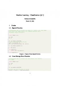
When using ICA to infer the labels of a directed graph G, the base classifier is used repeatedly to predict the label of a node given its content and neighboring labels. Since it is very rare to reach perfect classification, the base classifier of ICA often makes some prediction errors during inference. Since prediction errors become inputs for later classification problems, ICA raises an important bias between training and inference; in the former case, neighboring labels are always correct, while they may be noisy in the latter case. This training/inference bias is illustrated in Figure 2. The training/inference bias raised by ICA corresponds to a general problem that appears as soon as predictions become inputs for later classification problems. In the context of collective classification, the authors of Stacked Learning [8] identified the same training/inference bias. Both the Simulated ICA approach detailed below and Stacked Learning are motivated by the same concern: learning with intermediary predictions that are adapted towards the natural bias of the classifier.

Fig. 2. Illustration of the learning/inference bias of ICA. Left: during training, only perfect neighboring labels are considered. Right: during inference, several neighboring labels may be wrong due to classification errors.

4.1

Learning algorithm

In order to remove the learning/inference bias of ICA, the base classifier should be trained on situations representative of what happens during inference. In other words, the base classifier should be trained with corrupted neighboring labels. Furthermore, these labels should be biased towards the natural bias of inference: errors that are more frequent during inference should appear more during learning. Simulated ICA (Sica) relies on a simple, but powerful, idea to make training examples representative of inference behavior: simulation. We propose to simulate inference during learning, in order to create the training examples representative of the real use of the base classifier. The general scheme of the Simulated ICA learning procedure is given by Algorithm 3. Sica is an iterative learning algorithm which repeatedly runs ICA inference, using labels which are sampled based on the currently learned classifier P (yi |xi , N (xi )). This sampling operation can be performed in different ways, which are detailed in Section 4.2. At each inference step, one training example is submitted to the learning algorithm A, to train the base classifier for predicting the correct label yi given the node xi and the current neighboring labels. The key property of training examples in Sica is that they rely on currently predicted neighboring labels instead of assuming perfectly labeled neighbors, as it is the case of ICA. Similarly to classical ICA, both batch and stochastic learning algorithms may be used inside Sica. In our experiments, we used stochastic descent learning algorithm to update the parameters of the base classifier. 4.2

Sampling Methods

When learning with Sica, the aim of simulation is to generate a maximum number of situations that are representative of ICA’s inference behavior. Sica

Input: A labeled graph (G, Y ) Input: A multiclass learning algorithm A Output: A classifier P (yi |xi , N (xi )) repeat // Bootstrapping foreach xi ∈ X do yi ← argmaxl∈L P (yi = l|xi ) end // Iterative Classification repeat Generate ordering O over nodes of G. foreach i ∈ O do sample yi given P (yi = l|xi , N (xi )) submit training example ((xi , N (xi )), yi ) to A end until iterative classification terminates until learning has converged or a threshold number of iterations have elapsed return the classifier trained by A

Algorithm 3: Simulated ICA Learning algorithm

therefore relies on a sampling operation, whose role is to select the labels yi used during learning. We propose three sampling strategies: – Sica-Det (Deterministic) The simplest way to perform sampling in Sica consist in selecting the labels yi that are predicted by the current classifier P (yi |xi , N (xi )). Formally, the sampling operation used in Sica-Det is defined as follows: yi = argmax P (yi = l|xi , N (xi )) l∈L

– Sica-Uni (Uniform Noise) In order to increase the range of generated inference situations, one simple variant of Sica called Sica-Uni, consists in introducing stochasticity into the inference process by selecting labels randomly with a small probability. Formally, the sampling operation used in Sica-Uni is defined as follows: ( a random label l ∈ L with probability  yi = argmaxl∈L P (yi = l|xi , N (xi )) with probability 1 −  where  ∈ [0, 1] is a parameter controlling the tradeoff between random sampling and Sica-Det style sampling. – Sica-Prob (Probabilistic) Instead of using uniform noise, a more natural alternative consists in sampling labels from the P (yi |xi , N (xi )) distribution: yi = sample l ∈ L from P (yi = l|xi , N (xi ))

The advantages of Sica-Prob and Sica-Uni over Sica-Det are twofold. Firstly, stochasticity enables to generate a wider range of inference situations and thus creates more training examples for the base classifier. This may thus lead to more robust classifiers, especially when using few training nodes. Secondly, stochasticity may contribute to make training conditions closer to test conditions. In this sense, simulating the inference procedure with additional noise is an alternative to the cross-validation approach of Stacked Learning. In both cases, the aim is to learn with intermediary predictions that correctly reflect the behavior of the model on testing data. Stacked Learning creates the intermediary predictions by cross-validation, while we propose to directly modify the predicted labels on training data. We show in Section 5 that Sica-Prob and Sica-Uni frequently outperform Stacked Learning experimentally. 4.3 One classifier per pass ICA operates in several passes, where each node of the graph is re-estimated during one pass. Since the problem of first estimating the labels may slightly differ from the problem of re-estimating the labels at the second pass or at the third pass, the current pass number may have a direct influence on the base classifier. Instead of learning a unique classifier P (yi |xi , N (xi )), Sica can be modified to take the current pass number, t, into account, by learning a classifier P (yi |xi , N (xi ), t). Sica-Det, Sica-Uni and Sica-Prob can be modified by learning one distinct classifier per pass. This leads to three new variants of Sica that are denoted Sica+ -Det, Sica+ -Uni and Sica+ -Prob in the remainder of this paper. As an example, our experiments use Sica with 5 maximum inference passes, which leads to a set of 5 slightly different classifiers, each one specialized for a given inference pass. Concretely, using one classifier per pass makes it possible to learn finer inference-dependent behavior. This idea is similar to stacking: in both Sica+ and Stacked Learning, there is one classifier per inference pass and each of these classifiers is trained to compensate the errors of previous classifiers. Sica and Sica+ -Det perform both learning and inference in the same way. The only difference concerns the number of parameters which is multiplied by the number of inference passes by using one disctinct classifier per pass.

5

Experiments

In this section, we describe experimental comparisons between Simulated ICA and various state-of-the-art models for inductive graph labeling. 5.1 Datasets We performed experiments on seven datasets2 of scientific articles related by citation links and webpages from different universities related by their hyperlinks. 2

Datasets are available at http://www.cs.umd.edu/~sen/lbc-proj/LBC.html and http://www.cs.umass.edu/~mccallum/code-data.html.

Dataset Cornell Texas Washington Wisconsin CiteSeer Cora-I Cora-II

Nodes

Links Small scale – WebKB 195 304 187 328 230 446 265 530 Medium scale 3312 4715 2708 5429 Large scale 36954 136024

Features

Classes

1703 1703 1703 1703

5 5 5 5

3703 1433

6 7

12300

11

Table 1. This table shows different charasteristics (numbers of nodes, links, features and classes) of the seven different datasets used in our experiments. The four first datasets are small scale graphs from WebKB, the two following ones are medium scale graphs and the last one is our large scale dataset.

In these graphs, each node corresponds to a scientific article (resp. webpage) and each citation (resp. hyperlink) is represented by a directed link. Articles are described by feature vectors with one feature per word. Features correspond to most frequent words and indicate whether or not the associated words appear in the abstract of the article. Each dataset is composed of a graph and the aim is to categorize each node, in a multiclass setting. Table 1 summarizes several characteristics of these datasets, like the numbers of nodes, links, features and classes. The small and medium datasets were preprocessed by Getoor et al. (see [14] for more details). Cora-II was introduced by A. McCallum and was preprocessed by keeping only the words appearing in at least 10 documents. 5.2

Experimental Setup

State-of-the-art models In order to evaluate Simulated ICA, we have implemented three state-of-the-art graph labeling models: Iterative Classification (Ica), Gibbs Sampling (Gs) and Stacked Learning. Our implementation of Stacked Learning uses 5-fold cross-validation during learning to create the intermediary predictions. Stack2 is the simplest Stacked Learning model, where the labels are first estimated based on the content only and are then re-estimated by taking both the initial predictions and the content into account. Stack3 is a Stacked Learning model with three stacks: labels are first estimated using Stack2 and are then re-estimated with a classifier that uses both the content and the predictions of Stack2. Similarly, Stack4 and Stack5 are Stacked Learning models that respectively rely on Stack3 and Stack4 to provide intermediary predictions. Baselines We have also compared Simulated ICA with two baselines named Content-Only (Co) and Optimistic (Opt). The former is a classifier ignoring

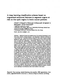
Fig. 3. A feature function to jointly describe content of nodes and neighboring labels. Feature vectors contain three parts. The first one describes the content of the node and the other two describe the labels of the node neighbors. For each label, there is a feature which counts the number of predecessor (resp. successors) with this label.

the graph structure and taking only the content of nodes into account during classification. The latter is a classifier which assumes the availability of perfect neighboring labels for each node, during both training and inference. Note that due to this dependency, the Opt baseline is not able to generalize to new unlabeled graphs and only provides an order of magnitude for the upper bound performance of graph labeling models. Base classifier In order to make the comparison fair, we used the same base classifier, the same learning algorithm and the same tuning procedure for all models. The base classifiers are L2-regularized maximum-entropy classifiers [4] learned with stochastic gradient descent. For each model, we tried ten different regularizer values and kept the best-performing ones. In order to take simultaneously the content of nodes and their neighboring labels, the base classifiers rely on a feature function that jointly maps contents and associated neighboring labels to scalar vectors. The feature function used in our experiments is illustrated in Figure 3. Data splitting In order to evaluate the generalization abilities of the models, we have split each dataset into one training graph and one testing graph. As [16], we have used a random sampling strategy: both the training and the testing graphs are random subsets of the whole graphs. When splitting graphs randomly, it is often the case that some links connect train nodes to test nodes. The simplest way to deal with these train-test links is simply to ignore them; this approach is called Test Links Only. Since many links may be discarded with the Test Links Only approach, we have also adopted an alternative approach proposed by [14] called Complete Links in which no link is suppressed and in which we assume, during inference, to know the correct labels of training nodes connected to testing nodes. Complete Links corresponds to the scenario where the input graph is partially labeled and the aim is to find the missing labels used in [14]

Co Ica Gs Stack2 Stack3 Stack4 Stack5 Sica-Det Sica-Uni Sica-Prob Sica+ -Det Sica+ -Uni Sica+ -Prob Opt

Cornell 71.79 72.91 73.02 73.02 73.02 73.02 72.91 73.53 74.24 74.04 71.48 72.71 73.42 72.5

Small scale – WebKB Texas Washington Wisconsin 82.14 80.52 85.21 82.46 81.22 84.76 82.67 81.04 84.98 82.35 81.74 84.38 82.46 81.13 84.76 82.67 81.3 84.83 82.35 81.13 84.76 82.24 81.83 85.21 83.21 82.35 85.36 83.42 82.43 85.74 80.32 80 83.32 82.35 81.13 84.45 82.35 81.91 85.06 82.78 82.17 84.46

Medium scale Cora-I CiteSeer 74.73 71.73 78.69 73.14 78.67 72.8 78.85 73.25 79.73 73.34 79.53 73.25 79.81 73.22 78.77 72.92 79.29 73.21 79.32 73.47 79.18 73.59 79.59 73.70 80.01 74.02 83.16 76.18

Table 2. This table shows the accuracy of different models on Cora-I, CiteSeer and the four WebKB databases. The graphs were split randomly into two folds by using Test Links Only strategy. We used 50% of the dataset as a training set and took the mean test accuracy over ten runs.

experiments. We kept it in a purpose of making comparisons. However, using this strategy with a 10-folds cross-validation appeared to be unable to deal with our assumption (since nine tenth nodes will be already correctly labeled), so we also ran a set of experiments with the Test Links Only approach by cutting the graphs into two folds. 5.3

Results

In our experiments, the parameters was the same as these in [16] for the baselines (Co, Opt, Ica, Gs and Stack): the maximum number of training iterations was set to 100, for Iterative Classification we used a maximum of 100 inference passes and for Gibbs Sampling we performed 1000 samples of each node label. For the Sica inference, we used a maximum of 5 passes. Moreover, we fixed the uniform noise percentage in Sica-Uni and Sica+ -Uni to 10%. Comparisons with state-of-the-art models We compared the six variants of Sica described in Section 4 with the baselines described previously on the small and medium scale datasets. Firstly, we have split each dataset into two halves by using the Test Links Only strategy. Each experiment was performed 10 times with different random splits and we report the mean test accuracies in Table 2. As expected, Sica models outperform Ica on all datasets. More interestingly, our models also outperform Gibbs Sampling and Stacked Learning in nearly all cases. In particular, the Sica-Uni and Sica-Prob models that rely on stochasticity outperform Stacked Learning on five datasets out of six, whereas this tendency is less clear for Sica-Det. As discussed in Section 4, adding a

Co Ica Gs Stack2 Stack3 Stack4 Stack5 Sica-Det Sica-Uni Sica-Prob Sica+ -Det Sica+ -Uni Sica+ -Prob Opt

Cornell 79.5 79.47 80.5 78.92 78.42 78.97 78.45 81.55 81.55 81.53 79.5 80.03 81.05 79.97

Small scale – WebKB Texas Washington Wisconsin 86.64 84.35 89.4 87.22 85.65 89.79 87.22 85.22 89.79 89.91 87.39 89.42 88.27 88.26 89.03 88.3 86.96 89.8 88.83 87.83 89.42 87.75 85.65 89.79 88.27 85.65 89.79 87.75 86.52 90.16 86.7 84.78 89.42 86.70 86.52 89.42 87.22 85.65 89.79 87.75 86.09 89.77

Medium scale Cora-I CiteSeer 77.43 72.98 88.52 77.63 88.18 77.47 88.07 76.72 88.18 77.35 88.4 77.23 88.4 77.08 88.37 76.27 88.26 76.48 88.37 76.33 88.74 77.75 88.63 77.93 88.66 78.02 88.85 78.08

Table 3. This table shows the accuracy of different models on Cora-I, CiteSeer and the four WebKB databases. Here, the graphs were split randomly into ten folds by using Complete Links strategy. Then, we did a 10-folds cross-validation and took the mean test accuracy.

perturbation to the predicted labels proves to be a good alternative to the heavy cross-validation based prediction process adopted by Stacked Learning. Among the two perturbation approaches, Sica-Prob most-of-time reaches better results than Sica-Uni. A deeper comparison of these sampling approaches in given below. Using one classifier per pass (Sica+ -Det, Sica+ -Uni and Sica+ -Prob) improves over the basic versions of Sica on the two medium scale datasets (+ 0.69% on Cora-I and + 0.55% on CiteSeer). On the small datasets, using one classifier per pass slightly deteriorates the results. We believe that this is due to estimation problems related to the large number of parameters on these approaches. The second set of experiments aims at comparing our results to those of [16]. Here, each dataset was split into ten folds by using the Complete Links strategy. Table 3 gives the 10-fold cross-validation accuracies (90% training nodes and 10% testing nodes) for all models and all datasets. As previously, our models most-of-the-time outperform Ica and Gs. On small datasets, Stacked Learning is competitive with our models. However, these results should be taken with a grain of salt, since, when using 90% training nodes with Complete Links, a large majority of testing-node neighbors are in the training set. Consequently, the various methods that take wrong labels into account during learning (Sica and Stacked Learning) have a more limited interest in this case. Impact of the uniform noise percentage Next, we evaluated the impact of uniform noise percentage on Sica-Uni. Figure 4 compares the three sampling methods on our two medium scale datasets. With a reasonable noise percentage

Accuracy

74.2 74 73.8 73.6 73.4 73.2 73 72.8 72.6 72.4 72.2 72

81 80 79 78 77 SICA+-Prob SICA+-Uni SICA+-Det ICA 0

20

SICA+-Prob SICA+-Uni SICA+-Det ICA

76 75 74 40 60 % Noise

80

100

0

20

40 60 % Noise

80

100

Fig. 4. Accuracy for varying percentage of uniform noise in Sica-Uni on CiteSeer (on the left) and Cora-I (on the right).

(below 40%), the accuracy of Sica-Uni is between that of Sica-Det and that of Sica-Prob. Once more, this confirms the contribution of stochasticity in the simulation process of Sica. In most cases, Sica-Prob outperforms Sica-Uni. Sica-Prob has another key advantage over the latter: it does not rely on additional hyper-parameter, which makes its tuning much easier. With a too high noise percentage, information in neighboring labels becomes irrelevant and thus accuracy drops down to the one of a Content-Only classifier. Large scale In order to show that our model can deal with large-scale graphs, we performed a set of experiments on the Cora-II database. For each model, we performed 10 runs with 20% training nodes and 80% training nodes selected randomly. The mean test accuracies are reported in Table 4. The first two columns give scores respectively for Test Links Only and Complete Links. The last two columns give the CPU time needed to train a single model and the time needed to fully label the test graph3 . Experiments were performed on standard 3.2 Ghz computer. Our approaches clearly outperform Ica and Gs on Cora-II (up to +3% improvement) and behave similarly to Stacked Learning with a much lower training time. Indeed, since each stack involves making 5 folds and learning a model on each sub-fold recursively, Stack models have a training time which is exponential w.r.t. the number of stacks. Instead, all our models – that use 5 inference passes – were learned in a few minutes.

6

Conclusion

In this paper, we have introduced the Simulated Iterative Classification Algorithm (Sica), a new learning algorithm for ICA. The core idea of Sica is to 3

Note that Sica models were highly optimized in our implementation, which explains their low training times.

Co Ica Gs Stack2 Stack3 Stack4 Stack5 Sica-Det Sica-Uni Sica-Prob Sica+ -Det Sica+ -Uni Sica+ -Prob Opt

Test Links Only 49 51.9 44.43 54.46 56.07 56.67 56.02 56.20 56.3 55.5 56.25 56.2 66.40

Complete Links 49 58.05 55.42 56.28 57.99 58.52 58.52 59.57 59.14 58.87 59.56 58.91 67.71

Training time 2 min 6 min 6 min 13 min 1h 4.5 h 20 h 5 min 3 min 3 min 5 min 3 min 2 min 3.5 min

Inference time 300 ms 20 s 10 min 1s 1.5 s 2s 2.5 s 4s 4s 4s 4s 4s 4s 600 ms

Table 4. Test accuracies and training/inference time on Cora-II. The first two columns give the mean test accuracy of the models with the Test Links Only and Complete Links splitting strategies. The last two columns show approximate training time and inference time. The results for Stack5 are incomplete due to the excessive time requirement of this method (since we average our results over 10 runs and try 10 different regularizer values, the experiment would need more than three months to complete).

simulate ICA’s inference during learning. We argued that simulation is a simple and efficient way to create training examples that are representative of real inference situations. We have shown that the proposed approach outperforms state-of-the-art models (Iterative Classification, Gibbs Sampling and Stacked Learning) on a wide range of datasets. Furthermore, we have shown that the model scales well, which makes it possible to label graphs containing thousands to millions of nodes. Our future work will primarily focus on generalizing the idea of simulation during learning to semi-supervised graph labeling problems. We believe that one promising approach is to develop (fast and scalable) incremental inference algorithms, that takes both the labeled and the unlabeled nodes into account, and to learn them using simulation. One key characteristic of ICA is that it relies on a classifier whose inputs depend on its previous predictions. Although this paper is focused on supervised graph labeling problems, we believe that the proposed idea of simulating inference during learning is relevant to a wider class of problems where predictions become inputs for later classification problems. In order to tackle error propagation problems in such algorithms involving classifier chains, simulation is a key solution, which appears to be both simple and efficient.

References 1. Jacob Abernethy, Olivier Chapelle, and Carlos Castillo. Witch: A new approach to web spam detection. Technical report, Yahoo! Research, 2008. 2. Shivani Agarwal. Ranking on graph data. In ICML 06, pages 25–32, New York, NY, USA, 2006. ACM. 3. Mikhail Belkin, Partha Niyogi, and Vikas Sindhwani. Manifold regularization: A geometric framework for learning from labeled and unlabeled examples. Journal of Machine Learning Research, 7:2399–2434, 2006. 4. Adam L. Berger, Stephen Della Pietra, and Vincent J. Della Pietra. A maximum entropy approach to natural language processing. Computational Linguistics, 22(1):39–71, 1996. 5. Carlos Castillo, Brian D. Davison, Ludovic Denoyer, and Patrick Gallinari, editors. Proceedings of the Graph Labelling Workshop and Web Spam Challenge, 2007. 6. Carlos Castillo, Debora Donato, Aristides Gionis, Vanessa Murdock, and Fabrizio Silvestri. Know your neighbors: web spam detection using the web topology. In SIGIR ’07, pages 423–430, New York, NY, USA, 2007. ACM. 7. Boris Chidlovskii and Lo¨ıc Lecerf. Stacked dependency networks for layout document structuring. In SAC, pages 424–428, 2008. 8. William W. Cohen and Vitor Rocha de Carvalho. Stacked sequential learning. In IJCAI, pages 671–676, 2005. 9. W. K. Hastings. Monte carlo sampling methods using markov chains and their applications. Biometrika, 57(1):97–109, April 1970. 10. R. A. Hummel and S. W. Zucker. On the foundations of relaxation labeling processes. pages 585–605, 1987. 11. David Jensen, Jennifer Neville, and Brian Gallagher. Why collective inference improves relational classification. In ACM SIGKDD ’04, pages 593–598, New York, NY, USA, 2004. ACM. 12. Zhenzhen Kou and William W. Cohen. Stacked graphical models for efficient inference in markov random fields. In SDM, 2007. 13. Frank R. Kschischang and Brendan J. Frey. Iterative decoding of compound codes by probability propagation in graphical models. IEEE Journal on Selected Areas in Communications, 16:219–230, 1998. 14. Qing Lu and Lise Getoor. Link-based classification using labeled and unlabeled data. In ICML: Workshop from Labeled to Unlabeled Data, 2003. 15. Sofus A. Macskassy and Foster Provost. Classification in networked data: A toolkit and a univariate case study. J. Mach. Learn. Res., 8:935–983, 2007. 16. Prithviraj Sen, Galileo Mark Namata, Mustafa Bilgic, Lise Getoor, Brian Gallagher, and Tina Eliassi-Rad. Collective classification in network data. Technical Report CS-TR-4905, University of Maryland, College Park, 2008. 17. B. Taskar, V. Chatalbashev, D. Koller, and C. Guestrin. Learning structured prediction models: A large margin approach. In ICML 05, Bonn, Germany, 2005. 18. Tong Zhang, Alexandrin Popescul, and Byron Dom. Linear prediction models with graph regularization for web-page categorization. In KDD ’06: Proceedings of the 12th ACM SIGKDD, pages 821–826, New York, NY, USA, 2006. ACM. 19. Dengyong Zhou and Bernhard Schlkopf. Regularization on discrete spaces. In Pattern Recognition, pages 361–368. Springer, 2005. 20. Dengyong Zhou, Bernhard Schlkopf, and Thomas Hofmann. Semi-supervised learning on directed graphs. In In NIPS, pages 1633–1640. MIT Press, 2005. 21. Xiaojin Zhu and Zoubin Ghahramani. Learning from labeled and unlabeled data with label propagation. Technical report, 2002.