Simulation of Driver Behaviour as a Function of Driver Error and Driver Daydream Factor
Kailash P. Thakur New Zealand Institute for Industrial Research, 24 Balfour Road, Parnell, P. O. Box 2225, Auckland, New Zealand. Email:
[email protected] Abstract: A driver-vehicle interaction model consisting of a closed loop system, developed recently, has been used to simulate the behaviour of drivers having different values of driver error and driver day dream factors. Concept of Risk Time, Driver Error and Driver Daydream Factors is presented and used to evaluate the vehicle-driver model. A process cycle of a driver-vehicle model is set up based on man-machine system theory. Crash conditions between two vehicles is presented, which can be used to design the intelligent control scheme for the highway system. When the risk time is large the normal driver is less attentive and the cycle time, defined in the driver model, becomes large. However, some drivers can have a cycle time comparable to the risk time. The value of the driver daydream factor, defined in the paper, becomes large for such drivers. The muscle response of such a driver is usually slower, giving rise to large values of the driver error in the driver model. The results for simulations of vehicle following another vehicle while changing the speed and driving under varying visibility conditions are presented. The computational results obtained have only logical and qualitative support; an exact quantitative comparison is not immediately possible. KEYWORDS: risk-time, human error, driver model, driver daydream factor, crash condition, perception, driver cycle, Nomenclature a
acceleration
k
Driver Daydream Factor
tD
decision time
tE
execution time
tH
human response time
tM
mechanical response time
tP
perception time
tR
risk time
T
total cycle time
u
initial speed
v
final speed 1
kmin
minimum value of driver daydream factor
kmax
maximum value of driver daydream factor
εmin
minimum value of driver error
εmax
maximum value of driver error
εr
reduced value of driver error
kr
reduced value of driver daydream factor
P
ratio of reduced diver error and driver daydream factor
2
1. Introduction Human factor in driving accounts for a large number of vehicle accidents today. The interaction between the vehicle and driver is very complex and depends upon several factors. This interaction changes with the driving situations, environment, time of the day, cognitive status of the driver and the duration of the journey. This paper addresses some of the issues of human factors in transport based upon a realistic driver model developed recently (White and Thakur, 1995; Thakur and White, 1996, 1997). The computer simulated results for a variety of drivers having different physical and cognitive capabilities are presented. The driver model (White and Thakur, 1995; Thakur and White, 1996, 1997) is described briefly in section 2. The result of simulation is peresented in section 3. 2. Driver Model Driver and vehicle interaction has been a subject of extensive study for the past few decades (Forster, 1991; MacAdam, 1980; Guo and Guan, 1993). The interaction between the known dynamics of the vehicle and unpredictable human behaviour is very complex. However, while human behaviour is not easily predicted, it can be estimated in a model for a normal person given certain constraints. 2.1 The driver -vehicle system The driver-vehicle system is considered to be a closed loop system as shown in Figure 1. Only four major points are considered on the continuous cyclic process: • Driver Perception. • Driver Decision. • Execution (path correction and/or speed control) and
3
• Mechanical Response of the system.
The cycle continues as Perception - Decision - Execution - Response Perception - Decision... as shown in Figure 1. The driver-vehicle system is a combination of mechanical and biological processes. The mechanical process is active only during the Mechanical Response phase of the cycle. Whereas, the biological processes are active during the Perception - Decision - Execution phases of the cycle. Figure 1 Driver Model Loop
This model of the driving process (or any other human controlled mechanical system) postulates that the driver’s task is separated into three parts, the perception of the current status of the mechanical system, the course and speed decision process and applying the driver inputs to the vehicle. Use of a closed loop system in drivervehicle interaction has been advocated by several investigators (eg. review by Guo and Guan, 1993; MacAdam, 1981). Rasmussen (1986) also describes a similar sequence of information processing in human-machine interaction system. Followed by perception, the output from the subconscious data processing system is always a 4
motor function, consisting of a great number of muscles that are controlled and coordinated by a complex, highly interconnected nerve system. The function of the mechanical system is only to transfer the driver’s control into output response. In the driver model loop, decisions will always lead to execution in the driver cycle, figure 1. At the point of execution in the driver cycle the execution is performed on the type and amount of manoeuvre required, which is a real number in the model having values positive, negative or zero. The zero magnitude is not ruled out by the present model and hence decisions may lead to any amount (positive, negative or zero) of execution. There is always some time involved in each phase on this cycle. The times are denoted by: tP, perception time; tD, decision time; including reaction time; tE, execution time, muscle activity; and tM, mechanical time, in converting control signals to an output by the mechanical system involving such elements as linkages, air pressure, and hydraulics in the vehicle.
Perception time and decision time depend upon the activity of the brain. During the human part of the cycle the mechanical system continues to operate with its control setting from the previous Execution phase. The total cycle time T is the algebraic sum of the individual times: T = tP + tD + tE + t M
(1)
5
The driver model assumes this loop is progressing continually (continuous cycling around this loop), with the driver perceiving the driving situation, deciding on control actions, executing the decisions by manipulating the driving controls and then the vehicle responding accordingly. In this analysis, tM is considered constant, depending only upon the mechanical system and is assumed to be short relative to the human response time. In practice, the mechanical response time can sometimes be long, catching out a novice driver who thinks the vehicle is not responding enough and overcorrects. This capability is not included in our present model. The values of parameters , tP, tD and tE can vary. These values can increase or decrease depending upon the driving situation, visibility, road conditions, and the driver. It is therefore possible to split up the cycle into two components, viz. 1. Mechanical part, involving time lag, tM, and 2. Human part, involving time tH, the algebraic sum of tP, tD, and tE.
Hence equation (1) reduces to: T = tH + t M
(2)
For a normal driver, the degree of concentration and alertness — and hence the human response time of the cycle — varies with road conditions (such as traffic density, type of intersections) and environment (including weather and visibility). Nagatsuka (1972, 1993) conducted several simulative experiments and found a gradual delay in choice reaction time and deterioration of performance. This delayed reaction time gives rise to variation in human response time in the driver cycle. Out of laboratory, numerous studies of car, truck and train driving have shown that the percentage of 6
slow alpha waves in the brain increase with time on the job, indicating a decline in alertness (Mackie and Miller, 1978; Kogi and Ohta, 1975, Hilderbrandt, et. al., 1975) giving rise to slow response. Drivers’ attentional response to environmental variations has been reported by Harms (1986, 1991). Based on the driver’s interpretation of the driving conditions, his/her own driving skill and the vehicle’s capabilities, the driver intuitively estimates the risk factor. On a divided highway with little traffic and good weather the risk factor is very small and hence the typical driver will not handle the controls so often and human response time tH is large. 2.2 Risk time We further define a time, tR, called Risk Time. This is the time after which, the driver thinks, the vehicle could reach “disaster” on the road. The Risk Time is estimated by the driver from the vehicle trajectory and anticipation of potential hazards or situations requiring corrective action. Such situations include: • hazard or traffic signal requiring the vehicle to stop; • vehicle following another vehicle keeping a safe distance or time lag; • hazard requiring an avoidance manoeuvre; • hazard beyond lane boundary requiring steering control to keep the vehicle in its designated lane.
For each situation a driver will estimate the time available before an avoidance action is essential. This Risk Time can be very small in some circumstances, for example a child darting onto the road.
7
A vehicle at high speed will have a relatively short Risk Time. Conversely, a vehicle at slow speed generally has a relatively long Risk Time. The Risk Time is limited by the driver’s visibility and anticipation. Van der Horst (1990) has used the time to impact (which is also known as time to collision) in several human factors studies to describe the temporal separation between vehicles when drivers start braking. The concept of ‘time to impact’ and ‘time to collision’ is similar to ‘risk time’ defied in this driver model. Human part of the cycle time (the sum of perception time, decision time and execution time) depends upon many factors, driving situation awareness, driver's individual capability, visibility, driver's training and experiences. The cycle time depends upon the risk time (White and Thakur, 1995), (a)
Large risk-time:
The driver does not stress much upon perceiving, deciding and executing the controls. The cycle time becomes large. If a child is darting on the road at 200 meters away from the driver’s car heading towards the child with speed of 10 m/s. The driver has 20 second at hand to avoid the risk of hitting the child. Driver can do a lot of manoeuvre in 20 seconds and he/she responds slowly (because the risk-time is large, his response is slow, and the cycle time is large in the driver model) (b)
Small risk-time:
If the risk-time is small the driver becomes cautious and he tries all his way to avoid the risk within the available risk-time. So his perception, decisions and executions are all very fast. The cycle time becomes small. If a child is darting on the road at 10 meters away from the driver’s car heading towards the child with speed of 10 m/s. The driver has only one second at hand to avoid the risk of hitting the child. Driver cannot do much in 1 second and he responds as fast as he could in order to avoid this
8
accident. (because the risk-time is small, the response becomes fast, and cycle time is small in driver model, in this case the driver is not relaxed as in case a).
If the driver is close to the risk (risk-time small) he has to act fast to avoid the risk. Higher is the risk the faster is the response. References can also be made to Carskadon and Dement, (1994); Rosekind et. al. (1993); and Dinges (1992) who talk about performance decrements that can be measured as a result of fatigue, which can impair information processing and reaction time and increases the probability of errors and can ultimately lead to accidents. This impaired information processing and reaction time gives rise to large values of human response time in the present driver cycle. The length of the human part of the cycle is dependent upon the Risk Time: as the Risk Time is perceived to decrease (indicating increasing risk of collision), the driver tends to concentrate harder. We assume that the human response time, tH, is proportional to the risk time. t H = kt R
(3)
The value of k in equation (3) depends upon the ability of the driver, which can vary between k = 0 to k = 1. For an expert driver the value of k, the Driver Daydream Factor, is small. For a novice driver, k is large. The parameter k is also related to the situation awareness factor. Relationship (3) has been experimentally verified for seven different road test experiments conducted on New Zealand roads (White and Thakur, 1995; Thakur and White, 1996). Fisher, Goodhall and Wark (1994) have demonstrated that information displays in cars may divert attention away from traffic environment giving rise to a large value of human response time. Laurell and Lisper (1978) have found a high correlation between reaction time and detection distance to
9
roadside obstacle. Reaction time of Laurell and Lisper (1978) corresponds to the human part of cycle time in the driver model and their distance to roadside obstacle corresponds to the risk time in this driver model and hence their study also support the validity of relationship (3). 2.3 Crash conditions If the Risk Time is less than the Mechanical Response Time, tM, the “disaster” will take place. If the Driver Daydream Factor, k, is large, there will only be time for a few cycles of the driver feedback process during the Risk Time available and any slight error, which are always present in such systems, can bring the system to disaster. If, on the other hand, k is small, that is, a good driver, there will be many cycles of the driver feedback process during the Risk Time. Any human error made in one cycle can be corrected in the next one and such a system will be a highly controlled one. Thus, the greater the number of cycles during the Risk Time the better (more reliable) is the control of the Human - Machine system.
2.4 Driving strategy There are many different driving control strategies. They include: • minimising journey time; • minimising distance travelled; • minimising fuel consumption; • minimising travel risk.
10
So far as the value of tH is concerned the human brain is very flexible — it can work relatively slowly in the relaxed state and very fast during an emergency. If the state of the brain is conscious, Perception Time and Decision Time are large. However, in the subconscious state of the brain, the perception and processing of information is fast (Forster, 1991; Rasmussen, 1986). Under such conditions, the minimum value of tH is limited by the Execution Time, since the muscle reflex is not as fast as the brain.
2.5 Driver error The driver is assumed to be imperfect. Driver errors in each phase of the human response cycle are possible. Human departure from the optimum performance is represented by the driver error. Errors in the mechanical system occur when the vehicle develops a fault. Mechanical faults are assumed to be negligible in this analysis and only the human factors are considered. Errors during Perception, Decision and Execution can be considered as one overall Human Error, represented by
ε. Human error, ε, varies from driver to driver depending upon their driving skills (training and experiences (novice cf. expert)). For the same driver, Human error, ε, also varies depending upon driving conditions, vehicle capabilities, cognitive workload and the duration of continuous drive, which accounts for driver fatigue. This error is reflected as driver input to the vehicle at the point of execution and hence becomes mainly of physical/muscular in nature. Human departure from the optimum performance has been explained in terms of external (task) and internal (psychological) conditions of the driver (Edwards and Tversky, 1976; Rasmussen
11
,1986). Human error is also reflected by the performance deterioration, examined by numerous investigators (Nagatsuka, 1993). The Driver Daydream Factor, k, is dependent upon speed of perception and judgement and is related to the mental state of the driver. Large values of k correspond to slow judgement. The Risk Time, tR, Driver Daydream Factor, k, and Driver Error, ε, work together to keep the system under control. If the values of ε and k are large and tR is small, the likelihood of system going out of control and a crash taking place is high. The Risk Time, tR, Driver Daydream Factor, k, and Driver Error, ε, are the fundamental parameters employed in this driver model. The driver model has been substantiated by experiments carried out for only one driving situation, ie, braking to stop (White and Thakur, 1995).
3. Driver Fatigue
Having defined and verified the driver model for a few realistic driving situations (White and Thakur, 1995; Thakur and White, 1996) we now proceed to use it for describing the interaction between vehicle and the fatigued driver. Fatigue is a general term commonly used to refer to the experience of being 'sleepy', 'tired' or 'exhausted' (National Aeronautics and Space Administration - NASA 1995). Fatigue can result in effects such as slowed reaction time and lack of concentration, as well as poor decision-making and worsened mood (NASA 1995).
Crawford (1961) pointed out the presence of two separate sources of fatigue in driving: first, the fatigue caused by driving itself (especially when it is for a prolonged 12
period); and second, fatigue from other sources such as (a) sleep loss, (b) circadian rhythm disruption, and (c) effect of other work performed before driving.
Brown (1994) and Crawford (1961) have noted the difference between muscular fatigue resulting from hard physical work (eg. labouring), and "skill fatigue", which is more related to the effect of prolonged concentration and vigilance in performing a fairly complex task like driving. The muscular fatigue, arising from physical work, as described by Brown (1994) and Crawford (1961) is called physical fatigue in this paper. However, "skill fatigue", arising from prolonged mental work as described by Brown (1994) and Crawford (1961) is called "Mental Fatigue" in this paper.
Poor decision making of a fatigued driver (NASA, 1995) gives rise to large error at the point of execution (large ε in the driver model). Slowed reaction time and lack of concentration of a fatigued driver (NASA, 1995) gives rise to large day-dream factor k, (ie. large value of the human response time according to equation (3)).
As issues of safety and health continue to be raised regarding fatigue in operational environments, more research will be required to address these concerns (NASA 1996). A major question raised in many operational settings is: What is safe?
Such issues
raised suggests a wide range of research activities. Performance decrements can be measured as a result of fatigue, which can impair information processing and reaction time (ie., large values of k) , which increases the probability of errors (large value of
ε) and can ultimately lead to accidents (Carskadon and Dement, 1994; Rosekind et. al. 1993; Dinges, 1992). Physical fatigue has been linked to physical work and overexertion (Mital. et. at., 1994). Klein and his colleagues (Klein, et. al., 1980) 13
synthesized the experimental work by Mackie and Miller (1978), who found that as driving time increased probability of accident involvement increased and lane tracking ability decreased. Stein, et. al. (1989) found that several accidents were the result of driver inattention resulting from fatigue. Driver performance decrements were correlated with fatigue by Stein (1995). Several studies have demonstrated that Reaction time increases with hours of continuous driving (Lisper, et. al, 1986). The lane tracking ability is due to the physical/ muscular capability of the driver reflected in Human Error ε in the driver model and inattention or increased reaction time is due to reduced cognitive involvement, which is represented by driver daydream factor k in the driver model.
Hence, the parameters of the driver model, the driver error, ε, and the driver day dream factor, k, permit us to account for a wide range of drivers having diverse capabilities including fatigue. The driver error, ε, is the error involved in the execution of the controls in the driver cycle. It is a representation of the physical (muscular) status of the driver. A physically sound, well trained and experienced driver will have a small value of driver error, ε, and he/she will be able to execute the controls with precision. However, a physically weak driver (even though he/she is well trained and experienced) will have a large value of driver error, ε. The driver day dream factor, k involves the perception, decision and situation awareness in general. Hence factor k represents the mental status of the driver and his ability to perceive the driving situation and make decisions. A small value of k refers to a mentally alert driver and a large value of factor k refers to mentally unalert (relaxed) driver. Hence fatigue in this model is considered to be of two different kinds, (i) physical tiredness, represented by a large value of ε and (ii) mental fatigue, 14
represented by a large value of factor k. This separation of fatigue into two components is also supported by Brown (1993) and Crawford (1961). In a normal person, mental fatigue gives rise to physical tiredness and vice versa. However, the extremes are also possible in typical individuals. 3.1 Following another vehicle under the “Two Seconds” rule Intelligent Transport Systems (ITS) have become a topic of considerable interest. The process of establishing and maintaining a desired range (gap) between a vehicle and the vehicle following it is of particular interest in developing an intelligent cruise control system (Fancher and Bareket, 1994). Until “intelligent cruise control” becomes a standard item fitted to automobiles, this job is carried out manually by the driver. It is worthwhile to look into this problem on the basis of the present driver model having a fatigued driver with varying degrees of fatigue. Figure 2 : Headway control problem
Range
Vehicle 1
Vehicle 2
Consider two vehicles (Figure 2) travelling with the same speed on a straight road separated by an interval of two seconds. (The New Zealand Road Code recommends that drivers remain at least two seconds behind any vehicle they are following). At a particular instant (say t = 0), the lead vehicle (vehicle-1) changes its speed with a constant acceleration a from initial speed, u to final speed, v. While trying to maintain a two second gap, the driver of the following vehicle (vehicle-2) also changes its speed. The Risk Time is the time in which vehicle-2 could crash into vehicle-1 under the current status of vehicle-2 (speed and acceleration). 15
The gap between the two vehicles, the time lag, and the speed and acceleration of the following vehicle change with slight fluctuations until a final steady state is reached with uniform speed v and constant time lag of two seconds. Time taken to reach the steady state depends on the magnitude of the speed change (v - u) and the acceleration level (a).
The computed results are presented for two cases: 1. reducing speed, v < u, 2. increasing speed, v > u. Table 1 : The values of parameters used in these computations Parameter
case (1)
case (2)
initial speed, u
150 km/h
60 km/h
final speed, v
60 km/h
150 km/h
acceleration, a (vehicle-1)
-2.0 ms
maximum possible acceleration of vehicle-2
4.6 ms
mechanical time, tM
0.002 s
maximum braking acceleration possible for vehicle-2
-5.0 ms
-2
-2
-2
-2
2.0 ms
4.6 ms-2 0.002 s -2
-5.0 ms
The vehicle parameters for this study are listed in Table 1. The behaviour of a normal driver with k = 0.2 and ε = 0.8 is represented in figures 3 and 4 for both cases, respectively. Figures 3 and 4 show the plot of range (gap) against range rate. These plots are of fundamental importance for ITS studies. During the slowing down or speeding up manoeuvres the curves in figures 3 and 4 circulates around the final equilibrium point in an elliptic path on range and range-rate plane. The dimensions of these “ellipses” could be very small if the values of k and ε are small. However, this 16
dimension could be very large for large values of k and ε. A situation might arise when range becomes negative at any point of time giving rise to a collision with vehicle -1. This situation can arise only if the values of k and ε in the driver model are large. It is not possible to conduct experiments with fatigued driver under the situation when the possibility of collision exists. However, it is always possible to carry out computer simulation to find out whether a collision is possible under the given situation or not. The simulation program was written to find out the minimum values of k and ε for which a collision is possible in cases 1 and 2. The region of safe domain generated by our simulation programme is shown in figures 5 and 6, respectively for cases 1 and 2. The permissible values of k and ε are contained within the safe domain. Figure 3
Range against range rate plot during
Figure 4 Range against range rate plot during the “speeding-up” manoeuvre
85
85
75
75
65
65
Range (m)
Range (m)
the “slowing-down” manoeuvre.
55
55
45
45
35
35
25
25 -8
-4
0
4
R a n g e R a te (m /s )
-2
0
2
4
6
R a n g e R a te (m /s )
17
Driver error (Physical)
Figure 5 Values of k and ε for which crash is possible in the slowing down process, case (1).
1.0 0.9 0.8 0.7
Unsafe Domain
0.6 0.5 0.4
Safe Domain
0.3 0.2 0.1 0.0 0.43
0.48
0.53
Driver Daydream Factor, k (Mental)
Fatigued Driver -------->
P(B) > P(C) > P(D) > P(E)
(9)
The value of P(C) = 1 at point C, indicates that the equal contribution comes from both sources, the physical tiredness and mental fatigue and this defines the normal form of fatigue, which has a maximum probability of occurrence. The measure of departure from normal fatigue (point C on arc ABCDE, Fig. 7) can be defined as
21
D( x ) =
arctan( P( x )) −
π
π 4
(10)
4
The value of D(x) varies from D(x) = -1 at point E to D(x) = 1 at point A on arc ABCDE. The value of D(x) = 0 corresponds to point C, the so called normal fatigue point on arc ABCDE. The value of D(x) in the range 0 < D(x) < 1 signifies that the origin of the current state of fatigue is due to physical reasons on the other hand the value of D(x) in the range -1 < D(x) < 0 indicates that the source of the current state of fatigue is the mental one. Figure 7 represents the key results for the investigation of interaction of a fatigued driver with vehicle and road. For a point x on the εr and kr plane (Figure 7), the distance r from the origin represents the measure of fatigue and the value of D(x) represents the nature of the fatigue.
The separation of physical and mental fatigue into distinct, orthogonal phenomena might look quite artificial. However, Brown (1994) and Crawford (1961) have noted the difference between muscular fatigue resulting from hard physical work (eg. labouring), and "skill fatigue", which is more related to the effect of prolonged concentration and vigilance in performing a fairly complex task like driving. The muscular fatigue, arising from physical work, as described by Brown (1994) and Crawford (1961) is named physical fatigue in this paper. However, "skill fatigue", arising from prolonged mental work as described by Brown (1994) and Crawford (1961) is called "Mental Fatigue" in this paper. Fatigue can result in effects such as slowed reaction time and lack of concentration, as well as poor decision-making and worsened mood (NASA 1995).
22
4. Future Research The present driver model involving the biological parameters ε and k is still far from perfect since it is not yet possible to determine/measure the values of the model parameters for a typical driver. Hence our further research will address the measurement of the driver parameters, and thus try to obtain behavioural and cognitive measures associated with the driving task. The measures used for the initial wide-spectrum assessment of motor and cognitive skills will be selected. Data acquisition protocols for these measures will be developed. Data collection will begin with a wide spectrum of motor performance and cognitive measures. The initial determination of motor skills and cognitive capabilities associated with risky versus safe driving will be based on the comparative performance of several drivers.
5. Conclusion Concept of Risk Time, Driver Error and Driver Daydream Factor is presented and used to evaluate the vehicle-driver model.
Based on man-machine system theory, a
process cycle of a driver-vehicle model is set up. A closed-loop driver model having a variable cycle time has been developed to represent the interaction between the vehicle and driver. Because each assumption made in the development of this driver model is supported by the experimental data available in the literature, the driver model is a realistic representation of the driving situations and so are the results generated by this driver model. Crash conditions between two vehicles is presented, which can be used to design the intelligent control scheme for the highway system. This model has been extended to represent the driver fatigue by means of the driver model parameters k, driver daydream factor and ε, the driver error. It is interesting to note in figures 3 and 4 that 23
the dimension of the ‘ellipse’ during slowing down manoeuvre is larger than that in speeding up manoeuvre. It shows that the performance of a typical driver is better during the speeding up manoeuvre than that during slowing down manoeuvre. Hence the same driver performs differently in different driving situations. The value of threshold fatigue which brings disaster on road is very much dependent on the driving situation (road conditions, such as traffic density, type of intersections, environment (including weather and visibility). The computational results presented in this paper have only logical and qualitative support; an exact quantitative comparison is not immediately possible. However, it does have some experimental verification in that the model has already been tested in some other driving situations. Hence, we expect that the other results, including the present ones generated by the model, to be realistic.
6. Acknowledgments The authors thank Mr. Peter Baas for encouragement. Thanks are also due to Dr. J. de Pont and Mr. Gary Bastin for critically reading the manuscript.
7. References Brown, I. D. (1994), Driver Fatigue, Human Factors, 36, 298-314.
24
Carskadon, M. and Dement, W. C. (1994). Normal Human sleep : An overview. In : M. Kryger, T. Roth and W. C. Dement (eds) Principles and Practices of sleep medicine, 2nd Ed. Philadelphia. Crawford, A. (1961). Tiredness and visual reaction time among young male nighttime drivers : A roadside survey, Accident Analysis and Prevention, 26, 617-624. Dinges, D. F. (1992). Probing the limits of functional capability : The effects of sleep loss on short-duration tasks. In R. J. Broughton and R. Ogilvie, (eds) Sleep arousal and performance, Boston : Birkhauser-Boston, Inc. 176-188. Edwards, W. and Tversky, A. (1976). Decision Making. Baltimore; Penguin Books. Fancher, P. and Bareket, Z. (1994) ‘Evaluating Headway Control Using Range Versus Range-Rate Relationships,’ Vehicle System Dynamics, 23, 575-596. Fisher, S., Goodhall, J. and Wark, L. (1994). Effects of new technology in cars on driver attitudes and behaviour. Paper presented at the 23rd IAAP International Congress of Applied Psychology, Madrid, Spain. Forster, H. J. (1991) ‘Der Fahrzeugführer als Bindeglied zwischen Reifen Fahrwerk und Fahrbahn’ (‘The Driver as the Connecting Link Between Tyres, Chassis and Road’), VDI Berichte NR, 916. Guo, K. and Guan, H. (1993) ‘Modelling of Driver/Vehicle Directional Control System,’ Vehicle System Dynamics, 22, 141-84. Harms, L. (1986). Drivers’ attentional response to environment variations: Adualtask real traffic study. In A. G. Gale, M. H. Freeman, C. M. Haslegrave, P. Smith and S. Taylor (Eds.), Vision in Vehicles I, Amsterdam: North Holland, pp 131-138. Harms, L. (1991). Variation in drivers’ cognitive load. Effects of driving through village areas and rural junctions. Ergonomics, 34, 151-160. 25
Hilderbrandt, G., Rohmert, W. and Rutenfrantz, J. (1975). 12 and 24 hour rhythms in error frequency of locomotive drivers and the influence of tiredness, International Journal of Chronobiology, 2, 175-180. Kageyama, I. and Pacejka, H. B. (1991) ‘On a new driver model with fuzzy control,’ Symposium of 12th IAVSD, pp. 314-324. Klein, R. H., Allen, R. W. and Miller, J. C. (1980). Relationships between truck ride quality and safety operations: Methodology development. Hawthorne, CA: Systems Technology, Inc. (NTIS: DOT HS 805 494) Kogi, K. and Ohta, T. (1975). Incidence of near accidental drowsiness in locomotive driving during a period of rotation, Journal of Human Ergology, 4, 65-76. Laurell, H. and Lisper, H-O (1978). A validation of subsidiary reaction time against detection of roadside obstacles during prolonged driving, Ergonometrics, 21, 81-88. Lisper, H-O. and Laurell, H., and van Loon, J. (1986). Relation between time to falling asleep behind the wheel on a closed track and changes in subsidiary RT during prolonged driving on a motorway, Ergonometrics, 29, 445-453. MacAdam, C. C. (1980) ‘An Optimal Preview Control for Linear Systems,’ J. Dyn. Sys. Measur. Control, 102, 188-93. MacAdam, C. C. (1981). Application of an optional preview control for simulation of closed-loop automobile driving, IEEE Transections on Systems, Man and Cybernetics, SMC-11 (6), 393-399. Mackie, R. R. and Miller, J. C (1978). Effects of hours of service, Regularity of schedules, and cargo loading on truck and bus driver fatigue, Goleta, CA: Human Factors Research, Inc. (Report 1765-F).
26
Mital, A., Foononi-Fard, H, and Brown, M. (1994). Physical fatigue in high and very high frequency manual materials handling: Perceived exertion and physiological indicators. Human Factors, 36, 219-231. Nagatsuka, Y. (1972). Fluctuations of reaction time during continuous trials for 40 minutes. Tohoku Psychologica Folia, 30, 75-83. Nagatsuka, Y. (1993). Simulative experiments on the control of behaviour in prolonged reaction situations: Conditions of suppressing deteriorations of performance. Tohoku Psychologica Folia, 52, 62-75. National Aeronautics and Space Administration, Ames Research Centre (1995) Fatigue Resource Directory. (on line) at : http://olias.arc.nasa.gov/zteam/fredi/home-page.html National Aeronautics and Space Administration, (1996) Current Activities on line at : http://www-afo.arc.nasa.gov/zteam/fcp/FCP.current.html Rosmussen. J. (1986). Information Processing and Human-machine interaction : An approach to cognitive engineering., North-Holland, Amsterdam. pp-78-200. Rosekind, M. R., Graeber, R., Curtis, R. and Dinges. D. (1993). Crew factors in flight operations IX : Effects of planned cockpit rest on crew performance and alertness in long haul operations NASA Technical Memorandum 108839. DOT/FAA/92/24. Thakur, K. P. and White. D. M. (1996). "Development of Driver model to investigate fatigue", Proceedings of The Second International Conference on Fatigue and Transportation : Engineering, Enforcement, and Education (Fremantle, Australia): pp. 455-67,
27
Thakur, K. P. and White. D. M. (1997). "Development of Driver-vehicle model on 'risk-time' basis", Driver-Vehicle Interaction, in press. van der Horst, A. R. J. (1990) ‘A time based analysis of Road User Behaviour in Normal and Critical Encounters. Report, TNO Institute for Perception, Soesterberg, the Netherlands. White, D. M. and Thakur, K. P. (1995). ‘Stability in the real world - influence of drivers and actual roads on vehicle stability performance’, in Road Transport Technology-4 Ed. Christopher B. Winkler, University of Michigan, pp. 545.
28