Simulation of Load Balancing Algorithms for Discrete ... - Roland Ewald

Simulation of Load Balancing Algorithms for Discrete Event Simulations Diplomarbeit Universit¨at Rostock, Institut f¨ur Informatik

Submitted by: Ewald, Roland Birth date: August 28, 1981 (in G¨ustrow) Matr.-Nr.: 1200089 Tutor: Dipl.–Inf. Jan Himmelspach Advisors: • Prof. Dr. rer. nat. habil. Adelinde M. Uhrmacher (Universit¨at Rostock) • Dr. Georgios K. Theodoropoulos (University of Birmingham) • Prof. Dr. rer. nat. habil. Peter Luksch (Universit¨at Rostock) Date of submission: April 10, 2006

Abstract Efficiently simulating discrete-event models in a parallel and distributed manner is a challenging endeavour. On one hand, various factors, such as hardware infrastructure or model characteristics, have to be considered. On the other hand, there is a wide variety of algorithms which address subproblems of parallel and distributed simulation and whose performance depends on the application at hand. This work illustrates the resulting difficulties with respect to the development of parallel and distributed simulation systems for general purposes. It is reasoned to what extent a prior analysis could facilitate this task. Approaches to predict the performance of parallel and distributed simulation systems are discussed. It is argued that the simulation of such a simulation system is a feasible approach. This claim is underpinned by implementing SimSim, a sequential simulator to simulate parallel and distributed simulation systems. Then, SimSim is used to develop a load balancing algorithm for the simulation of PDEVS models. The algorithm’s performance is analysed using SimSim. Finally, the predicted performance is compared to the real performance of the algorithm when running in the simulation system James II.

Zusammenfassung Die effiziente parallel–verteilte Simulation von diskret–ereignisorientierten Modellen ist ein herausforderndes Unterfangen. Dies liegt einerseits an der Vielzahl der zu ber¨ ucksichtigenden Faktoren, wie z. B. der vorhandenen Infrastruktur und den Charakteristika des zu simulierenden Modells. Zum Anderen existieren bereits verschiedenste Algorithmen zur L¨ osung von Teilproblemen der parallel–verteilten Simulation, die je nach Anwendung Vor- und Nachteile aufweisen. Diese Arbeit illustriert die daraus resultierenden Schwierigkeiten bei der Entwicklung von entsprechenden Simulationssystemen. Es wird er¨ortert, inwiefern eine vorherige Analyse die Entwicklung von neuen Algorithmen vereinfachen kann. Verschiedene Techniken, die eine solche Analyse erlauben, werden diskutiert. Des Weiteren wird argumentiert, dass sich die Simulation von Simulationssystemen gut als Ansatz zur Analyse eignet. Dies wird durch die Implementierung von SimSim, eines sequentiellen Simulators f¨ ur parallel–verteilte Simulationssysteme, untermauert. SimSim wird anschließend zur Entwicklung eines Load Balancing Algorithmus f¨ ur die parallel–verteilte Simulation von PDEVS Modellen verwendet. Die Eigenschaften des Algorithmus werden mit Hilfe von SimSim untersucht. Schließlich wird der Algorithmus in das Simulationssystem James II eingebunden, und sein Verhalten wird mit den Vorhersageergebnissen verglichen.

CR–Classification (1998): I.6.3[Simulation and Modelling]:Applications—Load balancing, PDEVS; C.2.4[Computer-Communication Networks]:Distributed Systems—Distributed applications; I.6.8[Simulation and Modelling]:Types of Simulation—Discrete event, Distributed, Parallel; D.2.5[Software Engineering]:Testing and Debugging—Diagnostics, Debugging aids, Testing tools; G.2.2[Discrete Mathematics]:Graph Theory—Trees, Graph algorithms; K.6.3[Management of Computing and Information Systems]:Software Management—Software development, Software selection;

Key words: Performance Analysis, Performance Prediction, James II

Contents Index

5

1 Introduction 1.1 Preface . . . . . . . . . . . . . . . . . . . . . 1.2 Terminology . . . . . . . . . . . . . . . . . . 1.2.1 Basic Terminology . . . . . . . . . . . 1.2.2 Parallel and Distributed Simulation . . 1.2.3 Distributed Discrete-Event Simulation 1.2.4 Simulation Languages and Systems . . 1.3 Typesets . . . . . . . . . . . . . . . . . . . .

. . . . . . .

. . . . . . .

. . . . . . .

. . . . . . .

. . . . . . .

. . . . . . .

. . . . . . .

. . . . . . .

. . . . . . .

. . . . . . .

. . . . . . .

. . . . . . .

. . . . . . .

. . . . . . .

. . . . . . .

8 8 9 9 10 11 11 12

2 Background 2.1 The DEVS Modelling Formalism . . . . . . . . . . . . . . . . . 2.1.1 The Discrete-Event System Specification Formalism . . . 2.1.2 Extending the DEVS Formalism to support Parallelism . 2.2 Challenges for Distributed Discrete–Event Simulation . . . . . . 2.2.1 Synchronisation . . . . . . . . . . . . . . . . . . . . . . 2.2.2 Granularity . . . . . . . . . . . . . . . . . . . . . . . . . 2.2.3 Partitioning and Load Balancing . . . . . . . . . . . . . 2.2.4 Further Challenges . . . . . . . . . . . . . . . . . . . . 2.3 A Brief Survey of Distributed Discrete-Event Simulation Systems 2.3.1 James II . . . . . . . . . . . . . . . . . . . . . . . . . 2.3.2 PDES-MAS . . . . . . . . . . . . . . . . . . . . . . . 2.3.3 Other PDES Systems . . . . . . . . . . . . . . . . . . .

. . . . . . . . . . . .

. . . . . . . . . . . .

. . . . . . . . . . . .

. . . . . . . . . . . .

. . . . . . . . . . . .

. . . . . . . . . . . .

. . . . . . . . . . . .

. . . . . . . . . . . .

. . . . . . . . . . . .

. . . . . . . . . . . .

. . . . . . . . . . . .

. . . . . . . . . . . .

. . . . . . . . . . . .

. . . . . . . . . . . .

13 13 13 15 17 17 18 18 19 21 21 24 26

3 Predicting Simulation Performance 3.1 Analytical Approaches . . . . . . . . . . . . 3.2 Semi-Analytical Approaches . . . . . . . . . 3.2.1 Benchmark Analysis . . . . . . . . . 3.2.2 Trace-based Performance Prediction 3.3 Empirical Approaches . . . . . . . . . . . . 3.4 Why Simulate Simulations? . . . . . . . . . 3.5 Towards a Proof of Concept . . . . . . . .

. . . . . . .

. . . . . . .

. . . . . . .

. . . . . . .

. . . . . . .

. . . . . . .

. . . . . . .

. . . . . . .

. . . . . . .

. . . . . . .

. . . . . . .

. . . . . . .

. . . . . . .

. . . . . . .

. . . . . . .

. . . . . . .

. . . . . . .

. . . . . . .

. . . . . . .

. . . . . . .

. . . . . . .

. . . . . . .

. . . . . . .

. . . . . . .

. . . . . . .

. . . . . . .

. . . . . . .

. . . . . . .

. . . . . . .

. . . . . . .

. . . . . . .

. . . . . . .

. . . . . . .

. . . . . . .

33 33 37 37 38 40 41 44

4 SimSim: A Simulation Simulator 4.1 Additional Terminology . . . . . . . . . . . . 4.2 Requirements . . . . . . . . . . . . . . . . . 4.3 Shortcomings of the PDES-MAS Simulator 4.4 A Generic Model of PDES Systems . . . . . . 4.5 Design of SimSim . . . . . . . . . . . . . . . 4.5.1 Overall Composition and Core Classes 4.5.2 User Interface . . . . . . . . . . . . . 4.5.3 Plug-Ins . . . . . . . . . . . . . . . . 4.6 Implementation Details . . . . . . . . . . . .

. . . . . . . . .

. . . . . . . . .

. . . . . . . . .

. . . . . . . . .

. . . . . . . . .

. . . . . . . . .

. . . . . . . . .

. . . . . . . . .

. . . . . . . . .

. . . . . . . . .

. . . . . . . . .

. . . . . . . . .

. . . . . . . . .

. . . . . . . . .

. . . . . . . . .

. . . . . . . . .

. . . . . . . . .

. . . . . . . . .

. . . . . . . . .

. . . . . . . . .

. . . . . . . . .

. . . . . . . . .

. . . . . . . . .

. . . . . . . . .

45 45 46 47 49 52 52 55 56 57

3

Contents 5 A Load Balancing Algorithm for James II 5.1 Related Approaches . . . . . . . . . . . . . . . . . . . . 5.2 Requirements Identification . . . . . . . . . . . . . . . . 5.3 A Benchmark Model . . . . . . . . . . . . . . . . . . . . 5.4 Development of a Prototype Algorithm . . . . . . . . . . 5.4.1 Version 1: Identifying Parallelism . . . . . . . . . 5.4.2 Version 2: Integrating Computing Load . . . . . 5.4.3 Version 3: Adding Adaptivity to Model Dynamics 5.5 Possible Enhancements . . . . . . . . . . . . . . . . . . 5.6 Porting the Algorithm to James II . . . . . . . . . . . .

. . . . . . . . .

. . . . . . . . .

. . . . . . . . .

. . . . . . . . .

. . . . . . . . .

. . . . . . . . .

. . . . . . . . .

. . . . . . . . .

. . . . . . . . .

. . . . . . . . .

. . . . . . . . .

. . . . . . . . .

. . . . . . . . .

. . . . . . . . .

. . . . . . . . .

. . . . . . . . .

. . . . . . . . .

. . . . . . . . .

63 63 65 66 69 72 74 77 79 80

6 Results and Analysis 6.1 Experimental Setup . . . . . . . . . . . . . . 6.2 Simulated Performance Results . . . . . . . . 6.2.1 Granularity . . . . . . . . . . . . . . . 6.2.2 Parallelism and Migration Cost . . . . 6.2.3 Scalability . . . . . . . . . . . . . . . 6.2.4 Dynamism . . . . . . . . . . . . . . . 6.2.5 Analysing the Adaptation Mechanism 6.3 Comparison to Performance in James II . . . 6.4 SimSim’s Performance . . . . . . . . . . . .

. . . . . . . . .

. . . . . . . . .

. . . . . . . . .

. . . . . . . . .

. . . . . . . . .

. . . . . . . . .

. . . . . . . . .

. . . . . . . . .

. . . . . . . . .

. . . . . . . . .

. . . . . . . . .

. . . . . . . . .

. . . . . . . . .

. . . . . . . . .

. . . . . . . . .

. . . . . . . . .

. . . . . . . . .

. . . . . . . . .

81 81 83 83 87 87 89 89 91 94

7 Conclusions 7.1 Resume . . . . . . . . . . . . . . . . . . . . . . . . . . . . . . . . . . . . . . . . . . . . 7.2 Putting the Work in Context . . . . . . . . . . . . . . . . . . . . . . . . . . . . . . . . . 7.3 Outlook and Future Work . . . . . . . . . . . . . . . . . . . . . . . . . . . . . . . . . . .

96 96 98 99

. . . . . . . . .

. . . . . . . . .

. . . . . . . . .

. . . . . . . . .

. . . . . . . . .

. . . . . . . . .

Bibliography

101

Glossary

108

List of Figures

113

List of Tables

115

A Voting Scheme for Model Migration

116

B UML Diagrams of SimSim

117

C SimSim Screenshots

120

4

Index GP , 73 P , 72 Pchange , 68 Ts , 50 Tw , 50 Ur , 69 ∆δext T , 68 ∆δint T , 68 ∆msgSize , 68 ∆nextM sgT , 68 ∆reactionT , 68 branchF actor, 83 c, 78 cpi , 49 d, 71 fperf , 43 lbCost, 83 lbF requency, 83 migrationCost, 76 numOf Groups, 83 numOf LP s, 83 pi , 49 pref , 68 rounds, 83 timeSpan, 69 tu, 81 tuamt , 81 tuswt , 81

Preference Factor, 68 Round, 68 State Phase, 68 Breathing Time Bucket protocol (BTB), 26 Breathing Time Warp (BTW), 29 Busy Time, 59 Cellular Automata, 21 Change Parameter, 78 Client/Server Architecture, 64 Cluster, 20 Complex System, 41 Computing Power Factor, 49 Constraint, 70 Critical Path, 38 Cross-Over Point, 43 Dead-lock, 17 Depth-First Search (DFS), 74 Desired Migration Rate, 78 DEVS, 13 Select, 14 δcon , 16 δext , 13 δint , 13 λ, 13 *-Message, 21 Abstract Simulator Tree, 21 Closure Under Coupling, 14 Coordinator, 21 Coupling, 15 done-Message, 21 i-Message, 21 Imminent Model, 14 Influencees, 14 Influencers, 14 LB-Message, 72 Legitimacy, 14 PDEVS, 15 Port, 15 Root Coordinator, 21 Simulator, 21 ta, 13 Time of Next Event (TONE), 14 Topmost Coordinator, 21

Abstract Class, 53 Activity Count, 74 Agent, 24 Situated Agent, 24 APOSTLE, 26 Application Model, 45 Application Model Time, 45 Barrier Synchronisation, 30 Baseline System, 49 Batch Mode, 46 Batik, 59 Benchmark Model, 66 Current State Phase, 68 Group, 68 Group Manager, 68

5

INDEX Logical Process (LP), 11 Agent Logical Process (ALP), 24 Communication Logical Process (CLP), 24 Lookahead, 17

x-Message, 21 y-Message, 21 DPAT, 29 Entity, 9 atomic, 9 Event, 11 external, 13 internal, 13 Event Horizon, 26 Global Event Horizon (GEH), 26 Local Event Horizon (LEH), 26 Event Precedence Graph, 38 Event Queue, 21 Event Source, 54

Main Plug-In Class, 56 Migration Matrix, 75 Model, 9 Atomic DEVS Model, 13 Coupled DEVS model, 14 MPI, 27 Multi-Agent System, 24 Multiset, 16 Original (PDES) System, 45 Original Model, 45 OSI Reference Model, 50

Fossil Collection, 17

Parallelism Graph, 73 Parallelism Matrix, 72 PARSEC, 28 Partitioning, 18 PDES2 , 40 PDES-MAS, 24 CLP Tree, 25 ID Query, 25 Range Query, 25 Server CLP, 25 Shared State, 24 Shared State Variable (SSV), 24 SSV ID, 25 SSV Type, 25 Performance Function, 43 PHOLD Model, 42 Physical Processor (PP), 11 Physical Time, 9 Plug-in, 46 Polymorphism, 53 Post-Mortem Analysis, 38 Processor Utilisation, 34 Proxy, 23 PVM, 27

Gain, 74 Gain Region, 85 Garbage Collection, 17 Generic System Model, 49 Georgia Tech Time Warp (GTW), 27 Global Virtual Time (GVT), 17 Granularity, 18 Graph Colouring Problem, 73 Grid, 20 GTW Blocking I/O Event, 27 Cache Coherent Multiprocessor, 27 GVT Thrashing, 27 Hardware Model, 49 Hiding Communication Cost, 71 High Level Architecture (HLA), 20 Host Processor, 49 IDES, 28 Interactive Mode, 46 James II, 21 Proxy, 23 Reference, 23 JANE, 27 Java Bean, 48 Java Virtual Machine (JVM), 91

Receive Time, 59 Risk, 29 RMI, 23 Remote Object, 23 Skeleton, 23 Stub, 23 Roll-Back, 17 Rounding Uniform Distribution, 69 Routing Algorithm, 20 Runtime Infrastructure (RTI), 20

Landau Notation, 35 Load Balancing, 18 Information Policy, 70 Placement Policy, 70 Transfer Policy, 70 Local Causality Constraint, 11

6

INDEX Scalability, 19 Scalable Vector Graphic (SVG), 59 Send Time, 59 Serialisation, 23 Setup Space, 43 SimSim, 45 Simulated Wallclock Time, 45 Simulation, 9 continuous, 11 discrete-event, 11 distributed, 10 parallel, 10 parallel and distributed discrete-event (PDES), 11 Simulation Space, 43 Simulation Time, 9 Slowdown, 10 Software Design Pattern, 53 Chain Of Responsibility Pattern, 54 Factory Pattern, 56 Observer Pattern, 56 Strategy Pattern, 53 Specific System Model, 49 SPEEDES, 28 Speedup, 10 SSF, 30 State Charts, 52 Straggler Event, 17 Synchronisation Algorithm, 17 conservative, 17 optimistic, 17 System, 9 System Model, 45 System Model Process, 53 TeD, 27 Time Unit, 81 Time Warp, 17 Trace, 38 Unified Modelling Language (UML), 52 Virtualisation, 40 Wallclock Time, 9 WARPED, 30 Workload Specification Language (WSL), 66 XML, 48 YADDES, 31

7

1 Introduction 1.1 Preface Prediction is very difficult, especially if it’s about the future. Nils Bohr As it has already been extensively used for the development of nuclear weaponry in the Manhattan Project, Modelling and Simulation is one of the oldest application areas of computers. Since those days, it has been applied to a broad variety of problems, from consumer behaviour in a supermarket to astronomical phenomena. Consequently, different modelling formalisms emerged to facilitate the model specification for certain domains. The major distinction between today’s models is whether they model an aspect of reality in a continuous way (e.g. by using differential equations) or by employing a discrete view. There are also hybrid approaches that combine both paradigms [65]. Discrete models are to some extent an abstraction of continuous ones, because they are restricted to a finite number of state changes within a time interval. Although there are differing views on discrete models [19], they can basically be regarded as a number of entities that notify each other of events by exchanging messages. As these so-called discrete-event models are the underlying principle of all discrete world views, this thesis is focused on discrete-event models. With the diversification of model specifications and world views, different simulation algorithms have been proposed. Today, the list of requirements for state-of-the-art simulation systems is quite long: At first, a distributed and parallel execution is often useful, because the models become more and more complex. Besides that, interoperability or the integration of external processes are, among other issues, of importance. Especially the efficient distributed simulation leads to a number of new problems. These problems (synchronisation, load imbalance, etc.) are common for all distributed software systems, but their solution has to be suitable for the context of a simulation system. To address these problems, various algorithms have been developed by the modelling and simulation community over the past years. This trend leads to an increasing complexity, because a simulation system can be designed as any reasonable combination of these algorithms. Moreover, different applications, execution platforms, programming languages and modelling formalisms make simulation systems even harder to compare and evaluate. Problems also arise when parts of an existing simulation system have to be enhanced or revised: A new algorithm may possibly evoke side-effects that strongly influence other parts of the simulation system. To overcome these issues, one could test the simulation system as much as possible. Unfortunately, this approach cannot resolve all problems (e.g. the platform and programming language dependency) and is rather laborious, especially when developing parallel and distributed simulation systems, which need a set of computers for each run. In this thesis, I will argue that a feasible approach to solve the above-mentioned problems is to apply modelling and simulation techniques on themselves: Since one of the main application areas of modelling and simulation is to gain deeper knowledge of modelled systems, modelling and simulation of simulation systems could possibly facilitate their development, testing and comparison. To illustrate this claim, I describe the simulation-based development of a load balancing algorithm for James II, a fairly complex simulation system which is developed at the University of Rostock: Firstly, I generalize an existing software for investigating certain aspects of the PDES-MAS simulation system, developed at the University of Birmingham and the University of Nottingham. This is described in chapter 4. Then, I model the relevant parts of James II and use the new tool, SimSim, to develop a load balancing algorithm for James II (chapter 5). Chapter 6 contains the analysis of SimSim’s simulation

8

1 Introduction runs, the incorporation of the gained knowledge into a real load balancing algorithm for JAMES II, and a comparison between its predicted and actual performance. Finally, I draw some general conclusions regarding the simulation approach, and give a short outlook to future research issues (chapter 7). Before this proof-of-concept is described, chapter 2 motivates the simulation of simulation systems in a more detailed manner. Several parallel and distributed discrete-event simulation systems are briefly described and compared, so that the complexity of the discussed problem becomes apparent. Additionally, other (and similar) approaches to predict simulation performance are presented in chapter 3.

1.2 Terminology This section clarifies the use of the most important technical terms in this thesis. For additional information, please refer to the index (page 5) or the glossary (page 108).

1.2.1 Basic Terminology System, Model, Simulation Obviously, these terms play a central role for modelling and simulation. Still, it is hard to choose from the dozens of proposed definitions, so the following ones have been picked regarding their usability in the context of this thesis. The American Heritage Dictionary defines a system as “A group of interacting, interrelated, or interdependent elements forming a complex whole.” [1, p. 832]. A model is described by Zeigler et al. as follows: “In its most general guise, a model is a system specification at any of the [system specification] levels [...].”[107, p.29]. Thus, models can be regarded as system specifications, and their behaviour can be simulated (i.e. computed) by a simulation software (see section 1.2.4). Often, modelling is used on systems that need to be investigated, particularly if interaction with the system itself is dangerous, expensive, or impossible. One way of investigation is to simulate a model of the system, which means that the model’s behaviour is calculated. This is usually done by a simulation system, on a computer. Afterwards, the simulation results are analysed, so that knowledge of the original system may be obtained. Since systems are composed of elements, it is natural that these elements are somehow reflected in models of them as well. Those element representations will be called entities. If a model contains representations of a system’s elements, it is possible to divide the model into several parts. This is evidently a requirement for its distributed simulation (see section 1.2.2). Similar to the elements of a system, the entities of its model are related to each other by data dependencies. An indecomposable entity is called atomic. Consider the distributed simulation of a model for a vector: Each number could be seen as an atomic entity. Another entity of the model, e.g. representing the sum of the vector elements, would have a data dependency to each of the vector’s number entities. Generally, the limitation of models as being composed of entities and connections between them is still very generic and subsumes a huge variety of modelling formalisms. Notions of Time The time it takes to simulate a model can be measured and used to evaluate performance issues. On the other hand, models usually incorporate a notion of time, too. To avoid confusion when using the same word in ambiguous situations, different notions of time have been identified and named: • Physical time: The time of the system that is modelled. For instance, a model of a medieval town could cover a physical time from the 5th to the 15th century. • Simulation time: The simulation time denotes the actual representation of time during the simulation. The start year of the medieval town simulation, e.g. 476, could be denoted as ’0’. Thus, simulation time is an abstraction of physical time.

9

1 Introduction • Wallclock time: The real-world time in which the simulation is executed. Reconsidering the medieval town example, the year 1492 (physical time) could be represented as year 1016 (simulation time), and its simulation may finish after 2 hours and 20 minutes (wallclock time). Later on, additional notions of time will be introduced (see chapter 4). A more detailed description of these terms is presented in [36, p. 27 - 28]. Speedup The speedup of a simulation run is measured in relation to a preliminary run, so that the performance benefits of a certain algorithm or adjustment can be quantified. Speedup is the ratio of the preliminary run’s runtime to the runtime of the modified run. It is either given as a factor (a speedup of 1.9 means that the modified run was almost two times faster) or as a percentage (a speedup of 50% means that the modified run was 2 times faster). When the speedup is less than 1.0, it is also called a slowdown. Although speedup is the most common measure for the performance of a simulation system, other, more general aspects like the utility for its users could be taken into account as well (e.g. see [69]).

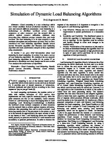
1.2.2 Parallel and Distributed Simulation The adjectives “parallel” and “distributed” are often used in conjunction, but they characterise different aspects of a simulation. That is, a distributed simulation does not necessarily need to be parallel, and vice versa. A parallel simulation processes a simulation experiment in parallel, i.e. it increases the performance by exploiting the “inherent parallelism” of a simulation experiment. This is useful if the execution of a single run takes too much time. Otherwise, if a single run can be executed fast enough but a large number of experiments has to be conducted, it would be easier to let each available processor independently execute a sequential simulation run. This way of parallelising a simulation is very powerful and easy to implement, but its use is restricted to the parallel execution of small-scale experiments. To speed up a single simulation run, a parallel simulation could concurrently calculate the parts of a model that do not depend on each other during a certain time interval. On the other hand, a distributed simulation system is executed on a set of physically distributed computers. Finally, if a simulation system fulfils both requirements, i.e. it allows the parallel execution on a distributed set of computers, we speak of a “parallel and distributed simulation system”. This thesis focuses on the efficient simulation of parallel and distributed discrete-event simulations (see figure 1.1).

Figure 1.1: Overview: Types of Modelling and Simulation. The red arrows and labels mark the topics that are covered in this thesis.

Additional information about the difference between distributed and parallel simulations, especially regarding the computer architectures they are executed on, can be found in [36, p. 17 et seqq.].

10

1 Introduction

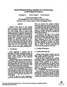
1.2.3 Distributed Discrete-Event Simulation As already mentioned in the preface, simulations are firstly distinguished by their modelling paradigm, whether they simulate continuous, hybrid or discrete models. Since this thesis focuses on discrete-event simulation, some related terms will be described here. Other types of discrete simulation, like timestepped simulation (e.g. used to simulate cellular automata), can be seen as special cases of discrete-event simulation. As Fujimoto states in [36, p. 34 et seqq.], an undistributed discrete-event simulation typically consists of state variables, a list of events, and a global clock value. The state variables represent the state the model is in. For each simulation loop, the event with the smallest time stamp is processed and removed from the list, which may result in a number of new events (with a time stamp greater or equal) and changes to the state variables. Subsequently, the global clock value increases to the minimum time stamp of the remaining events. This procedure continues until the event list is empty. Obviously, all events are processed in an increasing time stamp order. To ensure that the results of a distributed simulation algorithm are identical, this order has to be preserved. Otherwise, it would be possible that future events influence events in the past. This requirement is called the local causality constraint [36, p. 52]. To describe a distributed discrete-event simulation, Fujimoto [36, p. 40] uses Misra’s concept of logical processes (LPs) [64]: A logical process is an abstraction of a physical process that belongs to a distributed execution. Basically, each logical process is working like the undistributed discrete-event simulation outlined before: It manages a certain set of state variables and processes a list of events. In contrast to the undistributed simulation, the processing of an event may now result in the creation of events that cannot be processed locally, because they affect state variables that are managed by other logical processes. Therefore, all logical processes of a distributed simulation form a kind of logical network to exchange events among each other. In this network, only LPs that could exchange events are connected. Like in graph theory, all LPs that have a connection to a certain LP are called its neighbour LPs, or just neighbours. Since events are exchanged via messages, the terms event and message are often used synonymously in this context. The CPU that processes an LP is named the LP’s physical processor (PP). While an LP is executed on exactly one PP, each PP may execute multiple LPs. Another difference between distributed and undistributed simulation is the calculation of the global clock value. Contrary to undistributed simulations, the calculation of the global clock value is not straightforward for distributed simulations. Although each logical process stores a local clock value, which is the minimal event time stamp in its event list, the clock values of the other logical processes are unknown. Since the LPs ought to run in parallel as much as possible (to speed up the simulation), this leads to complications when deciding whether it is safe to process an event without violating the local causality constraint. To solve this problem, several approaches have been developed, which are briefly described in 2.2. Figure 1.2 sketches the basic structure of a distributed discrete-event simulation. Each LP maintains a local clock and a local event queue. Events to be processed by entities on a remote LP are sent over a network. To ensure the right execution order, each event contains a time-stamp and additional data. In this thesis, only parallel and distributed discrete-event simulations are considered. For the sake of readability, I use the common abbreviation PDES, or just the term simulation, to refer to them. Additionally, other discrete-event world views, like process orientation, can be built upon the eventoriented world view as described above. Nicol et al. characterise the event-oriented world view as follows: “While sparse, this paradigm is general enough to support construction of richer computational models, such as process orientation.”[71, p. 233]. Therefore, it is sufficient to concentrate on the event-oriented world view in the context of this thesis, without excluding the others.

1.2.4 Simulation Languages and Systems Finally, the term simulation system needs to be clarified. In general, as Low et al. state in [58, p. 171], one has to differentiate between simulation languages (e.g. APOSTLE [105]) and simulation executives (e.g. GTW [37]). While the latter are stand-alone systems that provide an interface for (model) applications and

11

1 Introduction

Figure 1.2: Scheme of a Distributed Discrete-Event Simulation

are comparable to libraries, simulation languages let the modeller define the model in a certain language and compile it - together with the corresponding simulation subroutines - to a single simulation program. Since this distinction is irrelevant for the actual execution, the term simulation system is used as an overall term for software systems that execute PDES.

1.3 Typesets Unless a term has just been emphasised by using an italic typeset, this indicates that it is mentioned for the first time, or that there is a glossary entry providing additional information. Besides that, “direct quotations” from other works are set in italic letters. As usual, monotype text refers to command line statements or fragments of source code.

12

2 Background This chapter aims at providing background information about parallel and distributed discrete-event simulation systems (PDES) in general. Before, definitions for different types of so-called DEVS models are given and explained. The DEVS formalism plays a central role for the next chapters. Then, major challenges for the efficient execution of PDES are described shortly. Finally, a brief survey of existing PDES systems is given. Owing to their relevance for the following chapters, the simulation systems James II and PDES-MAS are covered in a more detailed way.

2.1 The DEVS Modelling Formalism In this section, the Discrete-Event System Specification (DEVS) formalism will be described in detail. At first, I will describe the basic DEVS definitions (section 2.1.1). This will provide a good introduction to the modelling principles employed in DEVS. Afterwards, PDEVS, an extension to model parallelism of DEVS models, will be defined (section 2.1.2). This is a central topic, since the simulated load balancing algorithm will be tailored for PDEVS. An algorithm that can be used to simulate PDEVS models is presented in section 2.3.1. However, there are several other extensions of the DEVS formalism that will not be covered here (like DynDEVS [25], or Cell-DEVS [99]).

2.1.1 The Discrete-Event System Specification Formalism Definition of an Atomic DEVS Model The DEVS modelling formalism was developed by Zeigler [106] in order to provide a system modelling formalism that follows the principles of system theory. Consequently, the definition of DEVS models helps to ensure their system-like behaviour (e.g. explicit system borders, conditions for well-defined DEVS models, as described later). In principle, DEVS models can be seen as black boxes that only interact via a well-defined interface with their surrounding. Their internal behaviour is defined by a set of functions. The most basic DEVS model, the atomic DEVS model, is defined in [107, p. 138 - 139] as a tuple (X, Y, S, δext , δint , λ, ta) with X − set of p o s s i b l e inputs Y − set of p o s s i b l e outputs S − set of sequential states ta : S → ta(s), the model would have triggered an internal event before, which explains the definition of Q. No output is generated when an external event occurs. Zeigler et al. also formulate conditions under which a DEVS model is well-defined as a system, which means that δint does not cause infinite recursions [107, p. 141 - 142]. This so-called legitimacy of a DEVS model ensures that the model cannot change infinitely between states for which ta is 0, since this would violate the discrete-event principle of a finite number of events during a time interval. Now, atomic models can be composed to more complex systems by using coupled models. A coupled model is basically a container for atomic or coupled models. It not just contains some models, but also defines their input and output relationships. From an external point of view, a coupled model has the same interface like an atomic model, so that coupled models can be nested arbitrarily. In fact, it is possible to specify an equivalent atomic model for any coupled model (i.e. its output is the same as the coupled model’s output, for any input). This property is called closure under coupling (see [107, p. 127 - 131, 151 - 152]). Zeigler et al. [107, p. 150] define a coupled model as a structure N =< X, Y, D, {Md }, {Id }, {Zi,d }, Select > with X − set of p o s s i b l e inputs Y − set of p o s s i b l e outputs D − s e t o f r e f e r e n c e s t o t h e DEVS s u b m o d e l s i n {Md } ∀d ∈ D ∪ {N } : Id ⊆ D ∪ {N }, d ∈ / Id − s e t o f i n f l u e n c e r s f o r e a c h model and t h e c o u p l e d model ∀d ∈ D, i ∈ Id : Zi,d i s an i−to−d o u t p u t t r a n s l a t i o n w i t h : Zi,d : X → Xd , i f i = N Zi,d : Yi → Y , i f d = N Zi,d : Yi → Xd o t h e r w i s e Select : 2D → D − t i e −b r e a k i n g f u n c t i o n

The central part of a coupled model structure is the set of its sub-models, {Md }, and the index set D to reference it. Furthermore, data interchange between the models (including the coupled model itself, denoted by N ) is modelled by {Id } and {Zi,d }. An element Ix ∈ {Id } is a set of model references that defines all models whose outputs have to be propagated to the model Mx . Since Mx receives information from all models referred to in Ix , these models may influence the behaviour of Mx and are thus called influencers. This must not be confused with the term influencees, which stands for all models that Mx does influence by itself: inf luencees(Mx ) = {Mk |x ∈ Ik }. Hence, influencees have the opposite meaning of influencers, and are implicitly given in the definition. {Zi,d } is the output mapping of the coupled model. In general, it translates elements of the influencing sub-model’s output set to elements of the influenced sub-model’s input set. Without this translation, only models whose output and input sets are equivalent could be connected. However, the definition also contains two special cases: All inputs that arrive at the coupled model (N ) are mapped from X to the input set of the sub-models N influences. Correspondingly, the output of all sub-models that influence N is mapped to elements of N ’s output set Y . All in all, these mappings define the way the information is propagated within the coupled model. Finally, the internal state transitions of the sub-models have to be considered. For this purpose, the time of the next (internal) event (TONE) of each sub-model needs to be taken into account. The TONE of atomic models is defined by their ta function, whereas the TONE of coupled models is the minimal TONE of their sub-models. A model with a minimal TONE is called an imminent model. If there are more

14

2 Background than one imminent sub-models, the Select function is used for tie-breaking; it selects one of the eligible sub-models to execute its internal state transition. Since an internal transition could result in output, which then would be passed to the influencees of the model and cause them to process an external event, the Select function does not only specify the order in which sub-models with equal TONE should execute their state transition. Instead, a selection could also suppress the execution of internal events for eligible sub-models that were not selected (in case they are influenced by the selected sub-model). All in all, state transitions and input/output behaviour are completely covered by this definition. Therefore, a coupled model can be treated as an atomic model, which allows further nesting. To facilitate the specification and description of coupled models, some additional concepts are useful: Without loss of generality, it can be assumed that the input for a DEVS model contains information about the source of the input, and that the model output specifies a certain destination. Although these concepts are not explicitly stated in the given definitions, ways to identify different input sources and specify different output destinations can be easily added to any DEVS model. To facilitate the specification of coupled DEVS models, each model may define so-called ports for input and output1 .

Figure 2.1: Scheme of a Coupled DEVS Model

Thus, ports can be regarded as information sockets: output ports propagate certain model outputs, whereas input ports are used to receive certain inputs. A connection between the ports of two models is called a coupling. Each port can be part of multiple couplings, so that broadcasts can be modelled easily. The structure of a coupled model including ports and couplings is illustrated in figure 2.1.

2.1.2 Extending the DEVS Formalism to support Parallelism In [107, p. 261 - 284], some ways of executing the original DEVS models in parallel are discussed. However, Zeigler et al. also propose a modified definition of DEVS, PDEVS [107, p. 142 - 144], that aims at exploiting the inherent parallelism of a model. This means, the PDEVS formalism allows events that occur at exactly the same simulation time to be executed simultaneously. In other words, all imminent sub-models of a model are triggered to execute a state transition at the same time. A major advantage of this approach is that the synchronisation problem usually attached to parallel simulation can be avoided (see section 2.2.1 for details). The definition of PDEVS models differs only slightly from the original DEVS definition in section 2.1.1. Since all imminent models may realize a state transition at the same time, a coupled PDEVS model does not need a tie-breaking Select function. This is the most important difference between a coupled PDEVS 1 Actually,

DEVS models can also be defined by explicitly using ports (see [107, p. 84 - 86]).

15

2 Background

Figure 2.2: Comparison of DEVS and PDEVS. The leaves in the tree represent atomic models, which are incorporated into coupled models (i.e. their parent nodes). While the Select functions of the coupled DEVS models are used to determine the imminent model to be executed, all imminents are potentially executed in parallel when using the PDEVS formalism.

and a coupled DEVS model. In the original DEVS approach, the Select function selected one imminent model, which could execute its internal state transition safely. All models it influenced would perform an external state transition instead. Now, this distinction is not feasible anymore. The imminent PDEVS models cannot just perform an internal state transition in parallel, because it is possible that an imminent model is an influencer or influencee of another imminent model. This leads to two modifications of the original DEVS model definition: • Due to parallel execution, it might happen that a model receives multiple inputs (from all its imminent influencers). Therefore, input and output sets of atomic and coupled models have to be changed to multisets. A multiset (or bag) is a set that may contain an element multiple times (e.g. {a, b, b, b} is a multiset, with element ’b’ having a multiplicity of 3). • It is now possible that an imminent model has to execute an internal state transition (because it is imminent) and an external state transition (because there is some input from other imminents). To resolve this conflict, each atomic PDEVS model defines a confluent state transition function δcon to resolve this conflict. As for δint , a model is allowed to produce output in case of a confluent state transition2 . A major advantage of the DEVS formalism is that it strictly separates the models from the logic to execute them. This allows to plug in different kinds of simulation engines easily. One way to execute PDEVS models is described in section 2.3.1. Zeigler et al. also state in [107, p. 287], that the performance of a PDEVS simulation may be increased by not only executing imminent models, but models with a TONE that is almost the same as the minimal one. This extends the use of parallel PDEVS execution to situations where no inherent parallelism of the model can be exploited. However, this approach does heavily depend on the application and may lead to invalid simulation results if used wrongly. 2 Often,

δcon is defined as δcon (x) = δext (δint (s), 0, x), s being the current state of the model.

16

2 Background It is also possible to execute ordinary DEVS models in a parallel manner, as discussed in [107, p. 261 284], but this thesis will focus on the execution of PDEVS models.

2.2 Challenges for Distributed Discrete–Event Simulation This section presents some important fields of research regarding efficient parallel and distributed simulation. Actually, all of these problems can be traced back to similar problems that occur in all distributed software systems: many processes need some sort of synchronisation to interact in a meaningful way, load balancing and partitioning are considered as hard problems in the grid computing community (e.g. see [16]), and routing algorithms are a central topic for the networking community (e.g. see [74]). Nevertheless, the specific requirements of PDES often complicate the situations and call for suitable solutions.

2.2.1 Synchronisation As already described in section 1.2.3, the local causality constraint leads to the difficulty that each LP has to decide whether it can process its event with the minimal time stamp. This problem is addressed by synchronisation algorithms. In principle, there are two ways of ensuring event processing in an increasing time stamp order, which is sufficient to fulfil the local causality constraint: One possibility is to let each LP wait until it can be sure that processing the event with the currently smallest time stamp does not violate the increasing time stamp order, i.e. it is sure that it will not receive another event with a smaller time stamp. This approach is called conservative synchronisation. Another way of synchronisation is to let each processor process the events in its event list as fast as possible. Obviously, this can lead to violations of the increasing time stamp order, and thus of the local causality constraint. The key idea behind this so-called optimistic synchronisation is to detect these violations and correct them. To do so, the processors that processed events in the wrong order need to roll back to the state before the violation occurred. The violation of the time stamp order is detected when an LP receives a so-called straggler event. This is an event with a time stamp less than the local clock value. When this happens, the LP needs to be rolled back to the time stamp of the straggler event. Both synchronisation approaches bring some new difficulties: For conservative simulations (i.e. simulations that employ a conservative synchronisation scheme), the synchronisation algorithm has to define the situation in which an LP can be sure that no event with a smaller time stamp may reach it. Therefore, LPs have to somehow notify each other about the minimal event time stamps they could generate in the future. Usually, they do so by sending messages to their neighbours. A main goal of conservative algorithms is to minimise the amount of this notification messages. This is very important, because each LP has to be sure that none of its neighbours will generate an event that violates its time stamp order. This could lead to a large communication overhead. Furthermore, each notification should ensure safe event processing for as much time as possible. Modelspecific information can often be used to calculate an LP’s lookahead for a neighbour, which is the smallest time stamp of a new event the LP could possibly send to it. In fact, a good lookahead calculation is very important for conservative execution, because a large lookahead increases the chance that more than one LP can process its event list. A small lookahead also leads to another problem: dead-locks. A dead-lock is a situation, in which every LP needs a notification by at least one other LP to proceed. All LPs are blocking each other, and the simulation does never complete. Of course, this situation has to be avoided. There are several algorithms for dead-lock detection, and also techniques to entirely prevent them. Like the conservative simulation approach, an optimistic simulation introduces several new challenges. The basic idea of optimistically executing all LPs and letting roll-backs solve the rest is called the Time Warp algorithm [49, 34], which brings some serious performance problems. Firstly, the execution of roll-backs requires the storage of additional information, so that a former state can be restored. Consequently, a simulation with a large state may need huge amounts of storage. This problem can be solved by computing the global virtual time (GVT), which is the minimum time stamp

17

2 Background of any event in the simulation. The idea is that no LP can be rolled-back to a state before the GVT, because there is no potential straggler event with a small enough time stamp. GVT calculation by itself is not trivial, but there are several algorithms to compute this value (e.g. by Mattern [62]). Afterwards, the garbage (or fossil) collection of each LP can remove all information concerning states before GVT. Another major problem is that roll-backs often cascade. An LP that received a straggler event and was rolled back also has to invalidate all events it sent wrongly to other LPs. Often, this causes other LPs to roll back as well, and so on. This can greatly hamper the performance of the simulation. Although this phenomenon cannot be avoided in principle, it is possible to regulate the degree of optimism for each LP, so that faster LPs stop at some point and thus reduce the danger of being rolled back (see descriptions of the Moving Time Window approach [91], or its extension to the Breathing Time Warp approach [95], in section 2.3.3). Nevertheless, optimistic synchronisation has the big advantage of actually exploiting as much “inherent parallelism” as possible, whereas conservative simulation tends to be easier to implement and test. Interesting results are also achieved by combining conservative and optimistic approaches [23, 6]. A good overview of the most important synchronisation algorithms can be found in [36].

2.2.2 Granularity The granularity of a simulation can be understood as the ratio of the actual event processing effort to the overhead of sending it from one LP to another. This measurement is quite important, because it limits the possible speedup of a distributed execution. If events can be processed quite fast, but need a long time to be sent to another LP (i.e. the granularity is low), a distributed simulation could even execute much slower than a sequential one. Obviously, the granularity not only depends on the simulation experiment, but also on the hardware the PDES system is executed on: execution on a multiprocessor computer or on computers connected by a very fast network could drastically decrease the overhead of sending an event. Another way of increasing the granularity is to coalesce all events an LP sends to a certain neighbour. By this bundling, the overhead of sending a single event is reduced. For appropriate models, this approach may greatly increase the granularity, and thus the possible speedup. For example, Wonnacott et al. report a speedup of as much as 80% ([105], see section 2.3.3). On the other hand, this approach is not feasible for experiments where few events are sent to a large number of neighbour LPs.

2.2.3 Partitioning and Load Balancing Distributed simulation requires some additional mechanisms to ensure efficiency throughout the execution. At first, the model (i.e. its state variables) has to be distributed over all available LPs. Consequently, it has to be partitioned into several parts first. This might sound trivial, but a partitioning algorithm has to optimise the partition concerning two objectives: • Minimal Communication: The amount of data that needs to be exchanged between the LPs should be as small as possible. • Load Balance: Each LP should manage a part of the model that corresponds to its computing power. Both objectives are quite important, but it is very hard to optimise them in combination: For example, a partition that assigns the whole model to one LP would evoke minimal communication (nil, in fact), but this results in the largest load imbalance that is possible. On the other hand, it is possible to generate a perfectly balanced partition in which every LP gets its appropriate share of the model, but most likely with a huge communication overhead. This consideration leads to a basic question: How much load imbalance is acceptable in order to save a certain amount of communication load (or vice versa)? The answer to this question depends very much on the granularity, because communication overhead hampers the execution of low granularity simulations quite strongly, whereas load balance may be more important for simulations with a high granularity. Furthermore,

18

2 Background a large load imbalance could increase the number of roll-backs during an optimistic simulation: too lightly loaded LPs could receive an increasing number of straggler events from too heavily loaded LPs. The granularity itself depends on the model and the hardware used for the simulation (see section 2.2.2), so that a partitioning algorithm has to take all these aspects into account. Generally, partitioning could be seen as an optimisation algorithm that searches a partition p for which the function partitionobjective (p) = f actor · imbalance(p) + (1 − f actor) · communication(p) is minimal. By choosing f actor from the interval [0, 1], the importance of load balance can be weighted against the importance of communication avoidance. Exemplary mathematical definitions for functions to calculate imbalance and the amount of communication can be found in [29, p. 35 - 36]. However, most partitioning algorithms search for approximate solutions of the NP-hard partitioning problem, as it is known in theoretical computer science (a good survey can be found in [31]). Hence, they try to find an optimally balanced partition with minimal communication between the LPs, as opposed to approaches that optimise both objectives. Another research field deals with the development of load balancing algorithms for PDES. Since models may dynamically change their structure and computational demands, the partitioning of a model is not sufficient to ensure an efficient execution for longer simulation runs. Therefore, the simulation system has to adapt to changing communication and computation requirements, usually by moving parts of the model from overloaded LPs to underloaded ones. This is done by executing a load balancing algorithm that determines which model part has to be moved whereto. The development of a load balancing algorithm brings several new challenges: Firstly, the data that is needed to re-partition the model has to be gathered. This is not trivial by itself, because each measuring and calculation decreases the performance of the actual simulation. Secondly, the simulation system has to support the migration of model parts during the execution, which complicates the implementation (e.g. events may have to be forwarded to the LP which received the migrated model parts). Thirdly, the load balancing algorithm has to decide at which frequency an analysis of the collected runtime information makes sense: If the load balancing frequency is too high, the simulation performance is unnecessarily hampered by the execution of the algorithm. Is the frequency too low instead, the system is not able to react on sudden changes within the model. Due to this lot of problems and its rather tedious implementation, a load balancing algorithm is an ideal candidate to be tested via a simulation beforehand. A brief survey of load balancing techniques for PDES is presented in section 5.1.

2.2.4 Further Challenges As already mentioned at the beginning of this section, all distributed system requirements retain their validity and importance when developing distributed simulation systems. The following problems do not play a very central role for execution of a PDES in general, but may need consideration when developing a simulation system anyhow. This list is not exhaustive.

Scalability Scalability can be defined as the ability of a PDES system to cope with increasing problem size and an increasing amount of available hardware. In [68], Nicol investigated how model characteristics and partitioning affect the scalability of a PDES system. He also managed to define formal scalability requirements for a model, an architecture, and a PDES system (see section 3.1), but these requirements solely define upper and lower bounds. Moreover, they are hard to evaluate for most systems, so that scalability usually needs to be tested by hand.

19

2 Background Routing Algorithms As already mentioned, routing algorithms are of particular interest for the networking research community. Nevertheless, routing algorithms may also need additional consideration when developing distributed simulation systems. For example, if a simulation system subdivides the used LPs to fulfil different tasks. This is the case for the PDES-MAS simulation system, where some specialised LPs form a logical network to store a certain set of state variables efficiently. Other LPs have to generate special queries in order to access these variables. Since queries may also access sets of state variables at once, they need to be routed efficiently within the logical network (see section 2.3.2 for details). Interaction with External Processes Sometimes, simulations are used as a testing tool for hard- or software. Since analytical simulations should usually run as fast as possible, specialised synchronization mechanisms are needed to integrate external processes with a PDES system. For example, the wallclock time, in which the behaviour of an external process can be observed, has to be converted to simulation time. This allows to generate meaningful simulation events for the representation of the external process within the model. Otherwise, interaction between an external process and its (simulated) environment would depend strongly on the simulation speed, which in turn depends on the hardware etc., and thus would not be valid. Furthermore, simulation algorithms may have to be adapted to support waiting for external processes (e.g. see [45]). Interoperability and Reusability Since the development of valid computer models and simulation systems is quite expensive, efforts to increase the reusability and interoperability gain more and more importance. The most popular approach is the High Level Architecture [22], developed for the U.S. Department of Defense. The idea behind HLA is that simulation systems implement a pre-defined interface. Then, they are able to interact over the Runtime Infrastructure (RTI), which provides services of a distributed operating system and some additional functionality to support external processes and data collection mechanisms. In this way, simulation systems can be coupled and synthesised to form new applications. It is also possible to define custom data types (using HLA Object Models) that can be exchanged between different simulations. However, these requirements increase the complexity of simulation system development, because each stand-alone simulation system needs an additional interface that has to be tested and validated. Execution on a Grid The grid technology aims at providing computing resources as easy to use and flexible as the usage of the power grid [26]. This means, large applications are executed on a virtual supercomputer, which is actually a network of (normal) computers. This virtual supercomputer may be used by many users from remote locations, and with very different types of applications. Evidently, the execution of an application will be distributed over the available network nodes. This is not a new idea, but grid software usually combines several mechanisms like resource management, service discovery, and user management. Basically, grid software works as a distributed operating system for the concurrent execution of many distributed applications. The key advantage as opposed to literal supercomputers is the economical extensibility and setup of grid systems. Older computers may be integrated into the grid, as well as clusters or workstations with specialised hardware. All resources are managed by the grid system, which also ensures that only authorised users may start applications. Moreover, grid software has to provide mechanisms to recover from computer failures on certain nodes, so that a stable execution of an application is granted [46]. Although grid systems should facilitate the development of distributed applications, several considerations regarding the usually high latencies between grid nodes may have to be taken into account when developing algorithms for PDES systems [50].

20

2 Background

2.3 A Brief Survey of Distributed Discrete-Event Simulation Systems In this section, some sample simulation systems for PDES are introduced and described. This should illustrate that the problems mentioned in section 2.2 are indeed very common, and that several very different solutions have already been implemented. A more detailed survey of some PDES systems can be found in [58].

2.3.1 James II James II, the Java Agent Modelling Environment for Simulation, was developed by Himmelspach et al. [45]. It is a simulation system that aims at being highly flexible and efficient at the same time. It supports different modelling formalisms (e.g. Cellular Automata or DEVS) and a variety of simulation components to execute them. To date, James II mainly supports the efficient execution of different kinds of DEVS models. Additionally, James II allows to choose the set of simulation components that suit best to the model characteristics. For example, a certain simulation algorithm or event queue may have a huge influence on the performance. Other research aspects concern the reuse of model specifications [86] and the application of James II to various application areas (e.g. agent testing [39], intelligent tutoring systems [59] and bioinformatics [25]). All in all, the system is quite complex and integrates a variety of algorithms and simulation tools. In the following, the aspects of James II that are relevant for the next chapters will be described in detail. At first, an algorithm that simulates PDEVS models is outlined. Afterwards, I will give some relevant technical details about the way distributed parts of the simulation communicate with each other. The Abstract PDEVS Simulator in James II The PDEVS simulation algorithm by Chow et al. [20], which is used throughout this thesis to simulate PDEVS models, is called the abstract PDEVS simulator. A sample implementation is also given in [107, p. 284 - 287]. The James II implementation described here differs in some details from the original one, as it minimises the communication overhead. This will be explained later. The abstract PDEVS simulator consists of a hierarchy of individual components. Each atomic PDEVS model is associated with a simulator component, and each coupled PDEVS model will be executed by a coordinator component. The simulators and coordinators reflect the structure of a PDEVS model (as can be seen in figure 2.2), and thus form a tree, which is called the abstract simulator tree. The abstract simulator tree is similar to the tree of PDEVS models, except that each node represents a simulation component (i.e. a simulator or coordinator) instead of a coupled or atomic model. A special component in the abstract simulator tree is certainly the topmost coordinator. Its parent is the root coordinator, which controls the overall PDEVS execution. All in all, there are three different components that form an abstract simulator for PDEVS: the PDEVS simulator, the PDEVS coordinator, and the PDEVS root coordinator. The components of an abstract simulator tree are only communicating along its edges. This means, all communication is strictly hierarchical. Simulators only communicate with the coordinator of the coupled model their atomic model is part of. Coordinators only communicate with their parent coordinator and components that simulate direct sub-models. A model is only accessed by the component it is associated with. The abstract PDEVS simulator uses five types of messages, which are listed in table 2.1. At first, the root coordinator creates an i-message for the topmost coordinator, which then propagates it along the edges of the tree, towards each simulator (i.e. each leaf node in the abstract simulator tree). A simulator returns an i-message with the time advance function value of its associated atomic model. Hence, a coordinator is able to compute the minimal ta value of its coupled model’s sub-models. This minimal ta value can be seen as the ta value of the coupled model. It is propagated to the parent coordinator, which repeats this procedure. When the last answer to the i-messages reaches the topmost coordinator, i.e. it

21

2 Background Name i-Message *-Message x-Message y-Message done-Message

Use Initialisation of the simulation Activation of an imminent model Sending input to a model Sending output of a model Notification that a state transition is done Table 2.1: Message Types used by the Abstract PDEVS Simulator

has knowledge about the ta values of its associated model’s direct sub-models, it returns an i-message to the root coordinator and the initialisation is finished. Then, the root coordinator triggers a simulation step by sending a *-message (star message) to the topmost coordinator. The topmost coordinator will forward the message to all of its child components that have returned minimal ta values. Correspondingly, the *-messages will be propagated by all coordinators towards the simulators of the imminent atomic models. Now, the simulators of the imminent models have to let their models perform a state transition. However, at this point, a simulator is not able to decide whether it should let its model perform an internal or a confluent state transition. This is because all imminent models change their state in parallel, which makes it possible that an imminent’s output influences another imminent model. Obviously, the latter would have to perform a confluent state transition instead of an internal one. Therefore, the actual execution of a simulation step is divided into two parts. When receiving a *message, each simulator will only execute the output function on the current state (λ(s)). This is safe, since the PDEVS definition allows output for δint as well as δcon . Then, the model output will be sent as a y-message to the simulator’s coordinator. The main task for the coordinators is now to map the model outputs they received via the y-messages to model inputs, which then can be sent to the simulators as x-messages. This might sound trivial, but it is rather complicated. In general, a model’s output may have to be propagated through the whole tree. Due to the structure of a coupled model (see figure 2.1), an atomic model might produce output that will be propagated over the external output coupling of its coordinator. Thus, each output may have to be sent ’upwards’ in the abstract simulator tree. At the same time, when these outputs are eventually coupled with input ports, they can get ’downwards’ in the tree again, until they end up as input for an atomic model. All couplings in the PDEVS model define the destinations of a produced output, but each coordinator has only local knowledge of them, i.e. regarding the direct sub-models of its coupled model. To solve this problem in James II, each coordinator waits until all y-messages from sub-components that were triggered by a *-message have arrived. When this is finished, the outputs can be sorted, and a y-message with all outputs for the external output coupling is sent to the parent coordinator. Then, the coordinator needs to wait for external input. In James II, all inputs arrive in a single x-message. After including the external inputs to the internal inputs caused by outputs of its sub-components, the coordinator is able to allow each component to proceed with the execution. It does so by sending an x-message with all inputs to each component handling an imminent model, or a model that is influenced by one. If an imminent model is not receiving any input, an empty x-message is sent to its associated simulator component. Finally, the simulators may execute the second part of the simulation step. When receiving an x-message and the model is not imminent, δext is executed. If the model is imminent, either δint (the x-message is empty) or δcon (the x-message is not emtpy) are executed instead. Meanwhile, each coordinator waits for the done-messages from the components it sent an x-message to. When all components have signalised that they are done, a done-message is sent to the parent coordinator. Thus, the done-messages get propagated until they reach the root coordinator. Piggy-backed to a done message, each simulator and coordinator will send their new TONE values, so that the new imminents can be identified. In contrast to the other coordinators, the root coordinator will not propagate the done-message. Instead, it will either quit the simulation (when all TONE values are set to infinity) or send a new *-message to the

22

2 Background topmost coordinator. Thus, all in all, the abstract PDEVS simulator executes each simulation step in five phases: 1. Activation of all imminent atomic models by propagating a *-message top-down through the abstract simulator tree 2. Execution of all imminent atomic model’s output functions 3. Propagation of the outputs bottom-up and top-down to all influenced atomic models 4. Execution of the state transition, either δint , δext , or δcon 5. Notification of simulation step completion by sending a done-message bottom-up The main difference between the implementation presented in [107] and the solution used in James II is the way the delivering of a model’s output is realised. In general, it is not necessary for a coordinator to wait for the outputs of all sub-components, because each incoming y-message could be processed independently and sent to the parent coordinator if necessary. Correspondingly, each coordinator could process the external input. However, this results in a larger number of exchanged x- and y- messages, and thus in a larger communication overhead. In James II, each coordinator aggregates all messages, so that in any case only one x-message and one y-message are transferred between parent and child model. A major drawback of using the abstract PDEVS simulator is that the communication effort for one simulation step is quite large: in the worst case, if all atomic models are imminent, four messages are transferred for each edge in the tree (a *-, x-,y- and done-message). This could still lead to a huge overhead when distributing the simulation. Consequently, several other efficient algorithms to execute a PDEVS model have been developed. One idea is to flatten the abstract simulator tree [53]. This approach lets the root coordinator communicate directly to all simulators, which avoids latencies that occur when messages need to be propagated within a hierarchy. Communication between Simulation Parts Since James II is written in Java [48], which is commonly known as providing a good support for network applications, one could think that the communication between simulation parts is merely a technical detail. For example, Java programs may use Remote Method Invocation (RMI) to access Java objects on remote hosts. However, load balancing requires the ability to migrate parts of the simulation at runtime. By ’just’ using RMI, this is not possible, due to the way it enables the message invocation. An object that should be accessible by remote applications via RMI has to be the sub-class of a basic RMI object, like UnicastRemoteObject. Then, a so-called skeleton of the remote object is placed on the host from which it is accessed. The method calls to the remote object are handed over to the skeleton, which then forwards them over the network to the stub of the object. This stub serves as a proxy object (corresponding to the proxy pattern [38, p.207 – 217]) for the actual object. This means, it implements the same interface as the original object, and to call one of its methods will cause it to call the corresponding method of the object. Likewise, parameters and return values are forwarded. The stubs and skeletons of all remotely accessible objects have to be generated by the RMI compiler, rmic, beforehand. To migrate an object from one host to another, it has to be serialisable. In the context of object oriented network programming, serialisation means the conversion of an object to an array of bytes. After sending an object’s serialised representation over the network, the remote host is able to de-serialise it and to obtain the original object. Unfortunately, remote objects (i.e. objects that are remotely accessible) cannot be serialised like ordinary objects. Instead, the serialisation of a remote object results in its serialised stub, which may then be migrated. The real remote object, however, remains on the same host. One workaround would be to store the remote object’s data within a serialisable object and to send this object over the network. Afterwards, the new host of the object could create a new object and initialise it with the data object it received. The drawback of this approach is that the object re-creation might cause a certain overhead. Moreover, this method is quite complex to implement, as each object to be migrated has to provide additional methods for retrieving and setting the object’s state.

23

2 Background In James II, this problem is circumvented by an abstract communication layer, which also uses a proxy pattern [38, p.207 – 217]. Coordinators and simulators are not communicating directly with each other, but by using proxy objects. A proxy object stores the reference to a (remote or local) reference object that is able to access the object in question directly (see figure 2.3). To implement access to the reference object, one could even fall back on RMI or any other communication framework. In case of a migration, a simulation component can now be serialised and transferred, like all of its proxies to access other components. Only the relatively small and simple reference objects that allow remote objects to access the migrated component need special treatment. When using RMI, these objects have to be re-created on the new host, and all existing references to their old instances have to be updated.

Figure 2.3: Communication using intermediate Proxy and Reference Objects. Serialisable objects have a grey background. So, a component A and all of the proxies it uses can be moved to another host. Only the proxies used by remote components to access A still point to its old reference object, and thus have to be updated.

2.3.2 PDES-MAS The PDES-MAS simulation system (Parallel Discrete-Event Simulation of Multi-Agent Systems) [57] was developed by Logan, Theodoropoulos et al. to simulate systems of multiple situated agents efficiently. In this context, it is sufficient to regard agents as complex and partly autonomous objects. A situated agent is an agent that is embedded into an environment, which is part of the simulation. Usually, situated agents are able to move within this environment and do not have global knowledge about its state. However, they are able to sense some aspects of their surrounding within a certain range. In a multi-agent system, many agents are embedded into the same environment and interact with each other. Since even one agent might be rather complex and employ artificial intelligence methods, multi-agent systems may be extremely complex to develop. The PDES-MAS simulation system aims at facilitating the development of multiagent systems by providing an efficient platform to simulate them. This helps to gain deeper understanding of the systems, so that design decisions can be evaluated, and already implemented agents can be tested easily. Popular examples for multi-agent systems are Tileworld [80], Boids [85], or the Robocup Simulation League [84]. One problem of simulating multi-agent systems is that the state of the simulated model is usually quite large. Employing optimistic synchronisation techniques, as it is the case in PDES-MAS [55], even aggravates this issue, because some state saving mechanism is needed to support roll-backs (see section 2.2.1). The state of the simulation model can be divided into two parts: On one hand, there are private state variables for any entity of the simulated system (e.g. an agent). These variables cannot be accessed directly by other entities. Since only one entity is able to access these variables, they should be stored on the same host that executes the entity, so that a communication overhead is avoided. On the other hand, each entity might also incorporate public state variables that can be requested by any other entity. The set of all public state variables is called the shared state of the simulation, because

24

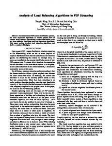
2 Background the shared state variables (SSVs) it contains may be accessed by any entity of the system. From the object-oriented programming perspective, the shared state variables are the result of a decomposition of (public) objects. To identify an SSV, each SSV gets a unique identifier, its SSV ID. Additionally, each SSV is associated with a certain SSV type, which represents class and field this SSV is an instance of. For example, the type of an SSV that stores the X-position of a box could be named Box-XPosition. As an example of a shared state, one could think of everything that is visible on a Robocup game’s virtual football pitch, whereas the plans of the competing football agents are private, and are therefore not part of the shared state. To manage the shared state efficiently, the concept of LPs is extended: PDES-MAS differentiates between agent logical processes (ALPs) and communication logical processes (CLPs). An ALP is a process that executes an agent and holds its private state. In contrast, a CLP manages a portion of the shared state. CLPs communicate with each other along the edges of a binary tree, the CLP tree. Each ALP is connected to a leaf node of the CLP tree, which is called its server CLP. The server CLP is the ALP’s interface to the shared state of the simulation. In general, the CLP tree can be seen as a distributed database system that is tailored to the needs of optimistic distributed simulation. This means, the CLPs do not only store the shared state, but they are also responsible for state-saving, as well as roll-back detection and execution. The structure of the CLP tree and the ALPs connected to it is shown in figure 2.4.

Figure 2.4: Structure of the CLP Tree

To access the shared state, an ALP creates a query and sends it to its server CLP. Clearly, different operations have to be supported. First of all, an ALP may need to read or write a single SSV. Hence, it issues a query that indicates the type of the access operation (i.e. read or write) and attaches the ID of the SSV it requests to access. The server CLP will resolve the query, potentially by propagating it through the CLP tree, and eventually return a reply message to the ALP. A query will be propagated if the current CLP is not managing the SSV to be accessed. Now, one challenge is to identify the CLP managing the SSV to be read or written, so that the query can be routed to the CLP along the edges of the CLP tree. This problem gets complicated when so-called range queries are supported as well: Basically, a range query resembles a selection statement of a rational database system. It requests the IDs of all SSVs that are of a certain SSV type and that have values within a certain range. This is particularly useful for the simulation of agents, because agents, as already mentioned before, usually do not have complete knowledge of their environment. Therefore, a situated

25

2 Background agent has to ’sense’ its environment to explore it. For example, an agent does not necessarily know all SSVs that represent box objects within its environment, nor does it know their SSV IDs. To get information about the boxes within its range (i.e. its direct surrounding), the agent issues a range query for the range it is interested in. As opposed to range queries, queries concerning only a single SSV are named ID queries. To solve the routing problem, two different routing algorithms have been proposed and evaluated [30]. Besides the routing problem for range and ID queries, the load of the CLPs has to be managed as well. This is done by an algorithm developed by Oguara et al. [73], which migrates the SSVs with respect to their access history. Using this mechanism, agents that frequently access a certain SSV may eventually ’drag’ this SSV to their server CLP. All in all, the PDES-MAS system is a simulation system that employs a set of sophisticated and specialised mechanisms to enhance the simulation performance for a certain class of models.

2.3.3 Other PDES Systems Now, several other parallel and distributed discrete-event simulation (PDES) systems and their main characteristics are presented briefly. The descriptions focus on each PDES system’s particular solution for the main challenges of PDES (as already described in section 2.2). All PDES covered here have been detailed in several research papers - which is, in fact, one of the reasons they have been selected. Furthermore, only PDES systems that are applicable for general simulation purposes have been considered. Other systems, which are restricted to simulate only particular types of models, were left out. For these reasons, the selection of PDES systems presented here is by no means representative. Nevertheless, the examples show the commonalities and differences between the described systems quite clearly. These will be summed up at the end of this section. APOSTLE The APOSTLE simulation system was developed by Wonnacott et al. [105] in 1996. It is built upon an optimistic simulator [104] and is actually a simulation language. For synchronisation, the Breathing Time Bucket (BTB) protocol was used [95]. This approach uses the notion of an LP’s event horizon. At first, each LP processes the events in its event queue and stores the newly created events locally. It proceeds until the minimum time stamp of the newly created events is less or equal to the next event in its event queue (events are processed in increasing time stamp order). When this happens, the local event horizon (LEH) of the LP is set to the minimum time stamp of the newly created events. Then, a protocol similar to those for GVT calculation can be used to calculate the global event horizon (GEH), which is the minimum of all local event horizons. All events that have been processed so far and have a time stamp not larger than the GEH are safe and can be committed. This means, they cannot be rolled back and all of their state information, which was saved for the case of a roll back, can be deleted. Only events with a time stamp between the global and the local event horizon have been processed in an optimistic manner and may be rolled back. Now, each LP sends out the newly created events that have been generated by committed events and are therefore safe to process. Some LPs might roll back towards GEH, because the events they received indicate a violation of the local causality constraint. Then, the same procedure continues. The research on APOSTLE regarding execution performance focused on the impact of granularity. The granularity of the simulation was reduced by coalescing a number of events before sending them, in one message, to another LP. Wonnacott et al. conclude that “APOSTLE’s granularity control mechanism will only give runtime reductions when, as a result of mapping multiple objects to the same LP, there are a reasonable number of simultaneous events for the LP itself.” [105, p. 120]. Thus, granularity control, for which Wonnacott et al. show that it is able to reduce the simulation runtime by as much as 80%, depends on the model’s characteristics and the ability of partitioning and load balancing mechanisms to provide a helpful object-to-LP mappping. Several simulation experiments with

26

2 Background different characteristics have been executed, for example a simulation of the Colombian health care system (as a queueing network) and a hardware simulation. GTW One of the most popular simulation executives in research is the Georgia Tech Time Warp (GTW) simulation executive by Fujimoto et al. [36, 37, 24]. At first, GTW was developed for cache coherent shared-memory multiprocessors. On a shared-memory multiprocessor system, multiple processors are connected via a bus and have access to a central memory. To avoid bottlenecks, each processor may be equipped with a cache to store data that is accessed frequently. In a cache coherent multiprocessor, each processor has a cache that ensures data coherency. This means, that a processor’s changes to data in its cache are immediately available for all processors accessing the same data. In other words, cache coherency makes caches transparent for the execution of concurrent processes that are accessing the same memory. GTW employs an event-oriented world view by providing a message interchange system between LPs. One goal of the GTW development was to create a high-performance simulator for models with a low granularity (i.e. with many events that can be processed without much computational effort). In a low granularity scenario, communication overheads have a huge influence on the overall system behaviour, since the processing of events can be done quite fast. The use of shared memory facilitates some problems of distributed simulation. For example, the GVT computation can be implemented straightforward using locks on global variables. Furthermore, the message passing can be implemented quite efficiently. Anyhow, GTW may be executed with different underlying communication layers, like PVM or MPI, as well [54]. GTW supports different optimistic synchronisation methods.This is achieved by allowing the creation of so-called blocking I/O events. Originally, blocking I/O events were used to synchronise the simulation with external processes, which usually involves input and output. The key property of these events is that they must not be executed optimistically. Instead, they may only be processed at GVT, which makes sure that they will be committed. This allows, for example, to output valid interim results during simulation runtime. A blocking I/O event causes the LP to stop processing any event until the GVT reaches its time stamp, whereas the non-blocking event, although not executed until GVT, allows the LP to process other events meanwhile. Different synchronisation schemes can be implemented by generating additional blocking I/O events. In [24], Das et al. also describe a phenomena named GVT thrashing. It occurs when an LP has advanced far ahead from GVT, and thus has filled the available storage with its event history. When no more memory is available, the LP will initiate a GVT calculation, so that its garbage collection can free some memory thereafter. When the garbage collection is not able to free a large amount of memory, since the GVT is still too small, the same LP will initiate GVT calculation over and over again. Obviously, this hampers the execution of the other LPs and thus the advance of the GVT, which results in a bad simulation performance. To avoid this problem, Das et al. introduce two parameters, Ff ree1 and Ff ree2 . They control at which point an LP is blocked, because it has too few memory left (Ff ree1 ), and at which (approximated) amount of free memory after garbage collection the LP becomes unblocked again (Ff ree2 ). Other memory management approaches, e.g. by generating artificial roll-backs, are described in [36, p. 137 -151]. Besides air-traffic control, GTW has also been used in the field of telecommunication. For example, it was used to simulate models in the network description language TeD [76]. GTW is supplemented by the JANE framework [77], which provides interactive simulation functionality. The integration of visualisation components is discussed in [18]. As for APOSTLE, the impact of granularity on the simulation performance was investigated [44]. For the simulation of PNNI, a network protocol for ATM switches, different partitioning schemes were evaluated [75]. A load balancing scheme was integrated into GTW, so that an efficient distributed simulation of dynamic models is possible [17]. Jiang et al. describe a framework that enhances the load balancing of GTW on the Grid [50].

27

2 Background IDES The Infrastructure for Distributed Enterprise Simulation (IDES) is a simulation system developed by Nicol et al. [71] at the Sandia National Laboratories. It is an optimistic simulator written in Java, focusing on portability and the execution in heterogeneous environments. IDES employs a slightly modified BTB protocol (see description of APOSTLE on page 26) for synchronisation, which is mainly characterised by a different calculation of the local event horizon (LEH). In IDES, all entities executed on one physical processor are regarded as being one LP. Thus, messages between entities on the same processor will be ignored for LEH computation. Instead of considering the time stamps of newly created events, the received messages from entities on other processors are used to calculate the LEH. With regard to them, the same synchronisation mechanism is used as in the BTB protocol: When the minimal time stamp of a received message is less than the next event to be processed, the event processing is stopped and the LEH is set to the minimal time stamp of the received messages. Then, the global event horizon (GEH) is calculated as usual, and all processors roll back to it. Now, each processor removes all received messages with time stamps greater than the GEH (because they are unsafe to process), and the same procedure can be repeated. Due to coalescing all entities on a physical processor and treating them as one LP, so that intra-processor messages are left out, the GEH calculated by this approach may be larger than the GEH calculated by the original BTB simulator. This advantage of a larger synchronisation window is somewhat hampered by the fact that it also increases the cost of state saving and makes roll-backs potentially more complex. Additionally, the size of the synchronisation window adapts to the available memory. When the amount of free memory is below a certain limit, the processor sets the time stamp of the last processed event as its LEH and stops processing. This corresponds to the memory control mechanisms in SPEEDES and GTW, as Nicol et al. point out, because “[...] the BTB window is the moral equivalent of GVT.”[71, p. 235]. Nicol et al. also estimated the cost of optimistic and distributed simulation by letting IDES run with and without those features on a single processor. When enabling state saving and synchronisation, the number of processed events per second dropped by approximately 30%. To better predict the performance of IDES, Nicol et al. also developed a performance prediction model [70] (see section 3.3). IDES was used for large-scale interactive simulations of nuclear weapon maintenance [5]. PARSEC The Parallel Simulation Environment for Complex Systems, PARSEC, was developed at the University of California by Bagrodia et al. [6]. Unlike many other PDES systems presented here (e.g. GTW or IDES), it employs a process-oriented world view instead of an event-oriented one. It is a simulation language based on C and a formerly developed PDES language, Maisie [8]. It consists of three parts: Parsec, the basic PDES system, Pave (Parsec Visual Environment), a user interface for Parsec, and finally Compose, which is a C++ library to facilitate the execution of parallel simulators. Besides that, PARSEC applications use the MPC (message passing kernel for C, [66]). Thus, a PARSEC application is actually a C program that uses some external libraries. This allows to migrate PARSEC applications easily from one platform to another. For synchronisation, PARSEC supports a broad range from conservative to optimistic protocols. Besides that, the use of different communication layers is possible (e.g. MPI or PVM). Finally, PARSEC incorporates several partitioning algorithms, which vary in their degree of automatism from user-controlled to fully automatic. It is, along with James II, one of the most flexible PDES systems in this overview. SPEEDES The Synchronous Parallel Environment for Emulation and Discrete Event Simulation (SPEEDES) was developed by Jeff Steinman [94, 95] at the Jet Propulsion Laboratory. Wieland et al. describe SPEEDES as “[...] a second generation Time Warp Operating System [...]”[101, p. 105] that “[...] benefited greatly from lessons learned during the development of TWOS [Time Warp Operating System].” [101, p. 105].

28

2 Background This means, SPEEDES aimed at resolving the performance problems that were caused by an overoptimistic execution. A first solution to this problem was the Breathing Time Bucket (BTB) protocol (as described in the section about APOSTLE, on page 26), which was originally designed for SPEEDES. Besides BTB synchronisation, Steinman also implemented the original Time Warp Algorithm and developed an new approach, Breathing Time Warp (BTW), that can be seen as a mixture of both [95]. Basically, the Breathing Time Warp protocol combines Time Warp and BTB by executing them alternately. Steinman presumes that the probability of an event to be rolled back increases the further it is ahead of GVT. Thus, BTW executes all events that are near the GVT like Time Warp does. But when a processor has processed N events, N being a user-defined parameter, it switches to the BTB phase and will not send out new messages anymore. When all processors have reached their local event horizon, the GVT will be calculated and the protocol starts over again. As Wieland et al. report in [101], SPEEDES employs a slightly different understanding of LPs and events: Here, LPs are just used as “data objects” to store the state, and they only provide basic functions to access it. In contrast, the main programming logic is situated in the event classes (SPEEDES is written in C++). Each event holds the code to process itself, including the scheduling of new events. Thus, the data objects are not simulation specific and may also be used as database interfaces etc.. The system is thereby divided into classes that contain the model semantics (i.e. the events) and classes that contain or provide the data the model is using. Wieland et al. evaluated the performance of different SPEEDES configurations with respect to a model of air traffic named DPAT (Detailed Policy Assessment Tool), which consists of a queue network that represents airport runways [101]. The DPAT model was executed using Time Warp, BTB and BTW synchronisation. Additionally, a sequential mode of SPEEDES has been considered. To study the influence of risk, which in the context of optimistic synchronisation techniques means the sending of messages although they might have to be rolled back, Wieland et al. introduce two parameters, Nrisk and Nopt . Clearly, Time Warp is a risky protocol, since all messages are sent right away. On the other hand, BTB is clearly a no-risk protocol, since no message is sent that could be rolled back later (recall that all messages are stored on the sending host until the global event horizon is computed). Now, Nrisk and Nopt can be used to fine-tune the BTW protocol. Each LP will stop its Time Warp phase after processing Nrisk events, and it will stop its BTB phase after having processed an overall number of Nopt events. Of course, if it reaches its local event horizon before it could process Nopt events, it will stop as well. If Nrisk = 0 and Nopt is set to infinity, BTW is equivalent to BTB. On the other hand, if both Nrisk and Nopt are set to infinity, BTW equates Time Warp. So, the behaviour of the protocol can be controlled seamlessly by varying Nrisk and Nopt 3 . Wieland et al. executed various simulation runs, with astonishing results: Surprisingly, the sequential DPAT simulation outperformed three of the four parallel approaches. Wieland et al. concede that the granularity of the DPAT model is quite low, and that the SPEEDES design seems to be suitable for sequential simulation as well. However, they also point out another implication: “The second implication is more foreboding: slow running extant sequential discrete event simulation models probably contain a lot of room for sequential performance improvements. If these performance improvements are made, then the case for running parallel is weakened considerably.” [101, p. 107]. In the case study, only BTW, used with Nrisk = 800 and Nopt = 3000 (which was the best setup according to Wieland et al.), brought a speedup of 2.1 on 9 processors. Nevertheless, several load balancing algorithms were integrated into SPEEDES and analysed for their use regarding the DPAT model [102, 103]. Additionally, Steinman developed an interactive version of SPEEDES [93]. 3 It

is assumed that Nrisk ≤ Nopt , otherwise the parameters would not make sense.

29

2 Background SSF The Scalable Simulation Framework (SSF) is actually not a PDES system, but a specification for which several PDES system implementations exist [21, 89]. The specification describes an API to create processes and events, and specifies interface declarations for C++ and Java. SSF is mainly used to simulate largescale networks. Basically, SSF can be used to implement sequential as well as parallel simulation systems. It supports a process-oriented world view, which also includes mechanisms for the event-oriented world view. One PDES implementation, named DaSSF, was developed by Liu et al. [56]. It is written in C++ and will serve as an example of this PDES approach. One of the most interesting aspects described in [56] is the performance prediction of DaSSF, which could be done with an accuracy of approx. 10% (see section 3 for more details). As a reason for performance prediction, Liu et al. argue: “We assert that the ability to accurate [sic] estimate performance without running a model is crucial to support rational software design, and can greatly boost one’s confidence that the effort one puts into model design will yield the desired performance gains.”[56, p. 1]. However, the performance prediction does not take load balancing into account, i.e. it assumes a perfect workload balance. According to Liu et al., this does not influence the prediction strongly, since the load balancing algorithms DaSSF provides are not costly. Clearly, this might not be the case for another kind of model, or another PDES system. Furthermore, the predicted results are only valid for an infrastructure with similar event queue implementation, computing power, etc., so that Liu et al. summarise: “We hope at some point to be able to automate much or all of this process; at present, to move to a different architecture is to require that the whole study be done once again by hand.”[56, p. 1]. Unlike the other PDES systems presented here, SSF only allows a conservative synchronisation approach. At first, all processors compute events within the system-wide minimal lookahead. Then, they synchronise using a barrier synchronisation (which only releases the processes when all have reached the ’barrier’) and send the generated events. Finally, all processes synchronise, again using barrier synchronisation, and repeat generating events within the lookahead.

WARPED WARPED is an optimistic PDES system developed by Martin et al. [60], in order to “[...] release a system that is freely available to the research community for analysis of the Time Warp design space.” [60, p. 1]. To motivate their goal, Martin et al. argue that former comparisons between different optimistic synchronisation protocols might be invalid, since “[...] these investigations are generally conducted in distinct environments with each optimization reimplemented for comparative analysis. Besides the obvious waste of manpower to reimplement Time Warp and its affiliated optimizations, the possibility for a varying quality of the implemented optimizations exists.”[60, p. 1] WARPED uses MPI as a communication layer. It has been developed in 1995, and was re-designed in 2003 [61]. The new version supports the possibility of runtime configuration and has a more modular architecture. While the first version did not include any partitioning or load balancing mechanisms, Subramanian et al. [96] provide a partitioning framework for the current version. Although all these efforts aimed at enhancing the comparability of optimistic PDES algorithms, Martin et al. concede: ”’Many groups have been (and are) working on various Time Warp optimizations and reporting results through various publications. Often there is no easy way to make direct comparisons between these optimizations. For example, many global time estimation algorithms for Time Warp have been developed [...]. However, since they have been developed in different systems, it is difficult if not impossible to make meaningful comparisons between them. At best, one must reimplement each optimization within their own system; at worst, a comparison is impossible due to architectural differences or resource limitations.”’[61, p.2].

30

2 Background YADDES The Yet Another Distributed Discrete Event Simulator (YADDES) is a simulation language developed by Preiss et al. in 1988 [81, 82]. It is based on C and was developed to compare different synchronisation protocols. In [81], the performance differences between optimistic and conservative synchronisation were evaluated, with strongly varying results that emphasized the impact of the simulated model. However, the simulation runs presented in [81] have been conducted on a single computer using parallel processes, so their validity is unclear. Preis et al. also show how the required transfer time of a message between two LPs can be estimated, although they have to make several very restricting assumptions in order to do so (e.g. computation and communication load are evenly distributed, and all computation and communication can be done in parallel) [81]. Summary Clearly, not all notable information about the PDES systems surveyed here could be given. Instead, I focused on the synchronisation protocols that have been implemented, since these were described exhaustingly in the corresponding literature. The various synchronisation protocols (BTB, BTW, etc.) were described to give an impression of the diversity and complexity of one of the PDES challenges mentioned in section 2.2 (albeit the probably most complex). Some theoretical background on load balancing will be presented in chapter 5. An overview of all aforementioned PDES systems is given in table 2.2 on page 32. Finally, this survey indicates some major methodological problems: • How can algorithms for PDES be compared conveniently? Many PDES systems (e.g. GTW) were designed to gain optimal speedup on a certain infrastructure. As Martin et al. point out in [61], this makes a fair comparison of approaches tedious or impossible (see description of WARPED, page 30). Moreover, the quality of different implementations cannot be guaranteed to be optimal. Consequently, although many of the surveyed PDES systems aimed at providing a comparison platform (e.g. WAPRED and YADDES), and there are many isolated comparisons of PDES algorithms (e.g. [7, 103]), these results may not be valid in general. On top of this, the lack of benchmark data regarding reference models makes a fair comparison virtually impossible. • How can we predict the performance of a PDES system? As can be seen in the survey, many researchers contributed new approaches to the field of parallel and distributed simulation. Some of them (e.g. Liu et al. for SSF [56] and Nicol et al. for IDES [70]) also tried to predict the performance of their systems. However, useful formulas could only be found when making very strong assumptions, or leaving out certain aspects that might be important (see section 3.1 for details). Of course, one could argue that there is no imperative need to predict simulation performance or compare different existing approaches: Instead, trial and error could be used to find the right solution for each simulation problem, even if this is costly. But considering the scientific entitlement of PDES research and basic scientific theory, the published results have to be falsifiable and repeatable. Indeed, the results are falsifiable and repeatable for their specific setup, but not necessarily in any other scenario, which obviously complicates their broad application. The numerous approaches to compare synchronisation protocols etc. show that this view is generally shared within the PDES community, and that a lack of these scientific prerequisites is recognised. Some approaches to overcome these difficulties are discussed in the next chapter.

31

32

C

Java

Java

C and C++

C++

C++

C++

C++

C

GTW

IDES

James II

PARSEC

PDES-MAS

SPEEDES

(Da)SSF

WARPED

YADDES

-

yes [96]

-

yes [102]

different rithms -

yes [29]

-

algo-

depending on the application

Partitioning -

-

-

yes [56]

yes [103]

yes [73]

-

under ment

-

develop-

yes [17, 50]

Load Balancing -

optimistic, conservative

optimistic

conservative

optimistic (BTW)

optimistic, conservative, or mixed optimistic

optimistic or conservative

optimistic (modified BTB)

optimistic, different approaches

Synchronisation optimistic (BTB)

large-scale networks [72] queuing networks, hardware hardware simulations [81]

air traffic [101], war games, etc.

wireless networks, hardware, etc. multi-agent systems

large-scale networks, interactive simulation agents [39], bioinformatics [25], etc.

Application hardware, health care network protocols, etc.

Table 2.2: Overview: A Selection of Distributed Discrete-Event Simulation Systems

Implementation C++

Name APOSTLE

-

additionally, problems of accessing shared data occur different world view: data and event objects based on SSF specification -

currently focusing on efficient simulation of DEVS models -

originally designed for cache-coherent shared memory processors -

Specifics granularity control

2 Background

3 Predicting Simulation Performance This chapter discusses possible solutions for the shortcomings outlined at the end of the last chapter, namely the comparability and predictability of PDES systems. As the chapter heading suggests, the focus will be on ways to predict the performance of PDES systems. However, some approaches also allow a fair comparison of PDES algorithms. The presented solutions range from analytical to empirical methods. At first, some purely analytical techniques are described, exemplified by a PDES model to analyse the impact of partitioning and synchronisation on scalability [68]. Then, different hybrid approaches, i.e. approaches that use mathematical methods and empirical data, are outlined. Afterwards, I give examples of empirical methods, which simulate PDES systems to predict their performance. Finally, I will argue why the simulation of PDES systems is a good option for predicting and comparing them. Possible problems that could hamper this approach are discussed, as well as additional benefits.

3.1 Analytical Approaches An interesting approach that highlights both problems and possibilities of analytical performance predictions was presented by Nicol in [68]. Here, I will sketch his attempt to define architectural and algorithmic requirements for a scalable PDES system. Nicol defines a mathematical model which then will be analysed and transformed. His model bases on the typical PDES idea of distributed simulation: The model to be simulated consists of entities, which are connected via channels. Additionally, he assumes that channels are uni-directional and have a non-zero delay d > 0, which means that the time stamp of a message sent through a channel has always to be greater than the simulation time of its creation1 . Now, λi is defined as the event rate of an entity i, which is the average number of all events associated with the entity, per unit of simulation time. In this context, association means that the event is managed by the entity, so that λi refers to the average event queue length of entity i. Correspondingly, µk is the average number of messages sent over channel k during one unit of simulation time. The N processors used by the modelled PDES system are assumed to be homogeneous, i.e. they all have the same computing power, network interface and storage. When partitioning the model, each entity has to be placed on one processor. So, the partition P can be seen as a mapping from the set of all entities into the set of all processors. Λj (P ) is the sum of event rates (λi ) for all entities that are mapped to processor j by the partition P . This model suffices to define some general ’cost’ measures, that actually determine the wallclock time needed to perform certain operations. Firstly, the cost of processing a single event is defined as X · log(Λj (P )), because Nicol further assumes that each processor has a single event queue. This event queue has the size Λj (P ), and it is assumed that the time to retrieve an event is proportional to log(Λj (P )). Since the event needs to be processed as well, and the mere proportionality between log(Λj (P )) and the time to retrieve the next event does not suffice to define the exact cost of accessing the event queue, log(Λj (P )) is multiplied by a “problem-dependent constant of proportionality”[68, p. 5], which is X. Secondly, the cost of sending an event is defined. The number of messages that are sent from processor i to processor j during one unit of simulation time is called the communication rate ci,j (P ). ci,j (P ) depends on the partition P , because it can be calculated by summing up the µk of all channels from entities on processor i to entities on processor j. Moreover, another proportionality constant M and the function 1 Although

this assumption is rather strong, Nicol argues that a model with zero-delay channels can be transformed into one without by aggregating events.

33

3 Predicting Simulation Performance a(N ) are multiplied to this term. While M is used the same way as X to ’calibrate’ the abstract rates to a physical system and thus reflects the network-related costs of sending a message, a(N ) is the function of the architecture size. This is introduced, because the scalability with respect to a growing architecture is one of the issues to be investigated. Therefore, a(N ) has to be proportional to the average number of network hops a message needs for getting from one processor to another. On top of this, possible contention due to architecture growth has to be modelled in a(N ) as well, whereas other contention effects can be expressed by adjusting M . Thirdly, a processor i that is receiving a message from processor j needs to insert the corresponding event into its own event queue, a cost that again will be proportional to log(Λi (P )). Again, a proportionality constant R will be multiplied with log(Λi (P )), so that the costs can be adjusted to match real-world circumstances. Using these cost definitions, the total execution cost for processor i during δ(P ), which is defined as a ’natural’ simulation time interval for which the costs are determined2 , is defined as

Ti (P ) ≤ δ(P ) · (Λi (P ) · X · log(Λi (P )) +

X

(a(N ) · M · ci,j (P ) + R · log(Λi (P )) · cj,i (P )))

(3.1)

j6=i

= δ(P )Ri (P ). As can be seen, δ(P ) is multiplied with the weighted sum of the three aforementioned cost components. Since processor i has to handle Λi (P ) events per time unit, the overall cost for processing events during one unit of time is Λi (P )·X ·log(Λi (P )). The processor will also exchange messages with other processors. This is expressed with the sum over all processors j 6= i: processor i will send ci,j (P ) messages to another processor j, which costs a(N ) · M · ci,j (P ) time, and will in turn receive cj,i (P ) messages from processor j, which amounts to a cost of R · log(Λi (P )) · cj,i (P ). The overall cost sum per unit of simulation time for processor i is denoted Ri (P ). Further, Nicol defines a ’bottleneck’ value Tmax (P ) = maxi {Ti (P )}, and correspondingly Rmax (P ) = Tmax (P ) δ(P ) , which is the cost sum for the bottleneck processor. If all parameters (i.e. a(N ), X, M , R) are adjusted correctly, Tmax (P ) defines the end time of the entire simulation for the given interval, since all processors are assumed to run concurrently3 . Now, synchronisation costs are added to the model. The synchronisation costs for one unit of simulation time are defined as S(P ), so the costs for an epoch of δ(P ) is δ(P ) · S(P ). Hence, the overall costs for simulating δ(P ) units of simulation time are Tmax (P ) + δ(P ) · S(P ). Nicol’s approach for testing whether a PDES setup is scalable bases on the notion of processor utilisation. In this context, it is the ratio of sequential simulation cost to the cost for using the PDES setup instead. Thus, it is a measure for the overhead induced by using parallel instead of sequential simulation: When then processor utilisation is rather high, i.e. it is only insignificantly smaller than 1 (the theoretical upper bound), there is negligible overhead due to parallel simulation, and one will achieve nearly linear speedup (e.g. a speedup of 4 using 4 processors). In contrast, a low processor utilisation indicates a high overhead. If the utilisation is lower than N1 , N being the number of used processors, a parallel simulation will even be slower than a sequential one. Therefore, processor utilisation is a good ratio to evaluate the performance of a PDES setup. P To define the cost for a sequential simulation of the same model, Nicol defines Λ = i λi as the overall event processing rate of all entities in the model. This can be used to approximate the event processing costs for a single processor. Therefore, a lower bound for processor utilisation U (P ) can be defined for a PDES system with N processors: 2 δ(P )

is only dependent on P for generality purposes, as Nicol states, so that different synchronisation and partitioning mechanisms might be evaluated using different analysis intervals 3 If this is not entirely the case, this can be expressed by adjusting the parameters.

34

3 Predicting Simulation Performance

δ(P ) · Λ · X · log(Λ) N · (Tmax (P ) + δ(P ) · S(P )) δ(P ) · Λ · X · log(Λ) = N · (δ(P ) · Rmax (P ) + δ(P ) · S(P )) Λ · X · log(Λ) = N · (Rmax (P ) + S(P )) U (P ) ≥

(3.2)

To investigate the impact of different parameters on the scalability of a PDES setup, one can now evaluate their impact regarding equation 3.2: if a parameter causes the lower bound to approximate 0, one can say that the PDES setup is not scalable regarding this parameter. Hence, Nicol defines a PDES setup to be scalable if the expression in 3.2 remains constant or grows when adjusting certain parameters. Next, he investigates the impact of architecture size and problem size on scalability. To do so, a growth function g(N ) is introduced. g(N ) specifies the number of model entities on the basis of the number of available processors. Nicol constraints the growth by three assumptions: (N )

1. For every entity i, λi = O( ΛN ), with Λ(N ) =

Pg(N )−1 i=0

λi

2. For every entity i, the sum of the µk on its outgoing channels is O(λi ) 3. Every message causes the scheduling of an event for the receiving entity The first constraint prevents the model from growing in such a way that a single entity has to process so many events that it overloads a processor, even if it is the only entity hosted there. Thus, as Nicol points out, ’serial bottlenecks’ for event processing are excluded. The second constraint relates the λi , which is constrained by the first assumption, to the number of messages an entity generates. Thus, a serial bottleneck regarding the sending of messages is excluded as well. Finally, the third assumption links the first assumption (bounded event processing rates) to the amount of received messages, so that serial bottlenecks are excluded here as well. The Landau notation (big-oh notation) used for the first two constraints expresses that the assumptions solely describe upper bounds. These assumptions are reasonable, because no PDES system would have a chance to scale when a single serial bottleneck (of any kind) is existent. Then, Nicol proves that every model that satisfies these constraints can be partitioned with a partition (N ) P 0 , so that the largest event rate of a processor is O( ΛN ) as well4 . Consequently, he introduces a constant (N )

c1 so that Λ00 ≤ c1 · ΛN , where Λ00 is – without loss of generality – the event rate of the most loaded processor. Now, given that the model also fulfils the second and the third constraint, which means that incoming (N ) and outgoing messages are also bounded by Λi (P 0 ), which in turn is bounded by c1 · ΛN , Nicol provides an upper bound for the cost of network communication known from equation 3.1: X

(a(N ) · M · ci,j (P 0 ) + R · Λi (P 0 ) · cj,i (P 0 )))

j6=i

≤ c1 ·

Λ(N ) Λ(N ) · (a(N ) · M · c2 + R · log(c1 · ) · c3 ) N N

(3.3)

Similar to c1 , c2 and c3 are constants for the second and the third assumption (i.e. bounds on message send and receive costs, respectively) that fulfil the upper bounds given by the Landau notation, for a (N ) sufficient large number of processors. Since every Λi (P 0 ) is bounded by c1 · ΛN (to fulfil the first assumption), and the second assumption has to hold as well, the number of outgoing messages for one 4 This

is rather technical, so the proof is left out here.

35

3 Predicting Simulation Performance (N )

processor (which has a finite number of entities) can be bounded by a constant c2 to c2 · c1 · ΛN . The same can be considered for the number of incoming messages and c3 . Now that an upper bound for each part of the maximal weighted sum of cost, Rmax (P 0 ), is known, this can be combined to: Λ(N ) Λ(N ) · log(c1 · ) N N Λ(N ) · (a(N ) · M · c2 + R · log(c1 · ) · c3 ) N

Rmax (P 0 ) ≤ X · c1 · +c1 ·

Λ(N ) N

(3.4)

Clearly, this inequality can be deducted from equation 3.1 by substituting Λi (P 0 ) by its upper bound (N ) c1 · ΛN , etc.. This enables the expression of a growth-dependent lower bound for the processor utilisation, by inserting the cost bounds into inequality 3.2:

U (P ) ≥

ΛN · X · log(ΛN ) N · (X · c1 ·

=

Λ(N ) N

· log(c1 ·

Λ(N ) N )

+ c1 ·

Λ(N ) N

· (a(N ) · M · c2 + R · log(c1 ·

Λ(N ) N )

· c3 ) + S(P 0 ))

ΛN · X · log(ΛN ) Λ(N ) · (X · c1 · log(c1 · =

Λ(N ) N )

+ c1 · (a(N ) · M · c2 + R · log(c1 ·

Λ(N ) N )

· c3 ) +

N ·S(P 0 ) ) Λ(N )

X · log(ΛN ) X · c1 · log(c1 ·

Λ(N ) N )

+ c1 · (a(N ) · M · c2 + R · log(c1 ·

Λ(N ) N )

· c3 ) +

N ·S(P 0 ) Λ(N )

(3.5)

This formula can now be analysed. For example, it is clear that the given bound will not approximate zero when only X is increased. So, if the granularity of our simulation is increased by making the processing of an event more complex in the average case, the lower bound for processor utilisation will never approximate zero. This implicates, that every PDES system scales with this kind of problem growth. However, as Nicol states, it may be that the synchronisation costs (S(P 0 )) rise as well, for example because state saving or roll-back costs increase when synchronising optimistically. Nevertheless, as Nicol further analyses the deducted formula, he finds some interesting relations. For example, he is able to prove the scalability of a simple conservative synchronisation protocol for a given architecture. The architecture assumption highlights the importance of efficient network topologies, because this could only be proven for a hypercube. The network diameter of a hypercube is very small, which makes a(N ) proportional to log(N ). Furthermore, Nicol describes the trade-off between synchronisation and load imbalance when the scalable synchronisation protocol is used. The protocol basically determines the minimal delay d (which is actually the look-ahead) for all channels between different processors, and then executes all events within a time window d. The larger the minimal delay of inter-processor channels, the larger is the synchronisation window that is used, and the smaller are the costs of synchronisation. Now, the partitioning algorithm could at first merge all entities that have a channel connection with a delay smaller than a given value d0 , and then partition the remaining entities. This would guarantee a synchronisation window size of at least d0 , but the partly merged entities may be harder to map evenly on all processors. Therefore, Nicol proposes a binary search algorithm to find the optimal relation of synchronisation and imbalance. All in all, Nicol’s approach is quite impressing: It demonstrates that mathematical modelling of PDES systems is very well possible, and that rather general and broadly applicable conclusions can be deducted. Having said that, it is evident that a thorough analysis of such a complex formula, with such a number of adjustable parameters (which even may depend on each other), is anything but easy. Even for this general approach, several strong assumptions have to be true, for example the execution of the PDES on a set of homogeneous processors, non-zero channel delays, and that the cost of accessing an event queue is proportional to log(N ). If one of these assumptions does not hold, the analysis has to

36

3 Predicting Simulation Performance be repeated. Since there are event queues whose access costs are O(1) under certain circumstances, Nicol points out that “Reduction of the event list cost is a sort of good news and bad news deal.”[68, p. 11]. On top of this, many of the used parameters are very hard to find out for existing PDES systems. For example, Nicol admits that “For most synchronization protocols, quantifying S(P ) is extremely difficult.”[68, p. 5], and that “Furthermore, synchonization behaviour is frequently complicated, which makes it very difficult to analytically prove anything about performance executing large models on large machines.”[68, p. 4]. Another restriction is the focus on average rates, so that the possibly dynamic behaviour of the model is not modelled explicitly. Consequently, additional costs, for example the cost of load balancing, are not modelled explicitly as well, and thus cannot be analysed directly. These examples illustrate the biggest shortcomings of the analytical prediction approach: The results, although being quite general, cannot be applied easily to real-world situations. Additionally, the mathematical models tend to be quite complex, and often base on rather strong assumptions. However, these assumptions have to be made, otherwise a mathematical model would not be tractable at all. So, the mathematical prediction of simulation performance is rather laborious, very sensitive to preliminary assumptions, and the results are often hard to apply. Owing to these difficulties, Nicol concludes that “[...] it becomes increasingly critical to establish whether PDES technology will scale up with increasing problem size and architecture. In this paper, we address the problem in a general setting, provide a resounding conclusion: maybe.”[68, p. 11]. Nevertheless, mathematical models have the strong advantage of being able to show theoretical upper and lower bounds in general, so that limitations in principle can be detected. There are several other analytical approaches, one of them was presented by Gupta et al. [43], who predict the performance of time warp. In contrast to Nicol’s approach, they do not search for a theoretical lower bound that can be analysed, but try to predict several performance measurements (e.g. speedup, number of roll-backs, etc.) for a time warp simulation. The resulting equation system was solved numerically, and the results were compared to real-world measurements. The comparison showed that the speedup prediction was rather good, only overestimating the speedup by at most 10%. But, again, the model implies several strong assumptions: For example, the analysis based on the fact that communication takes no time at all. While it is clear that inter-processor communication on the shared memory processor that was used to generate the real-world data might be negligible, this is surely not the case when using other network topologies. Actually, Nicol shows in [68] that network communication overhead does matter. Furthermore, other aspects of the problem, like dynamic model behaviour, load balancing, or granularity were left out. The equation system and its deduction were nevertheless quite complex and sophisticated. Altogether, analytical approaches may not be the best way to predict the performance of specific PDES systems. The next section presents some approaches that combine analytical considerations and real-world data to generate predictions more easily. Finally, the aforementioned examples indicate that it is generally quite hard to predict PDES performance. Some reasons for that are suggested in section 3.4.

3.2 Semi-Analytical Approaches 3.2.1 Benchmark Analysis Unlike purely analytical techniques, which focus on the analysis of rather general PDES system models, one could also enrich a mathematical method with benchmark data from existing PDES systems. This approach was used by Liu et al. to predict the performance of the DaSSF system, as already described in section 2.3.3 [56]. Basically, Liu et al. investigated execution times for low-level operations that had to be performed quite often when running a simulation with DaSSF. Then, the occurrence of these operations was calculated by a straightforward mathematical model. By putting the measured execution times of the operations into the mathematical model, the execution time could be predicted. The prediction quality was rather good for most predictions (approx. 10% deviation), but in some cases it varied by as much as 30% from the real-world execution time.

37

3 Predicting Simulation Performance To gather useful benchmark data, Liu et al. identified several operations that are essential for the performance of DaSSF. Since they implemented an own threading mechanism, the speed of switching the context (i.e. switching the process currently executed) had to be measured. Different experiments were designed to examine the average execution time for different blocking functions. Moreover, the costs of creating process and event objects were evaluated. Finally, they quantified the costs of accessing their event list implementation and of possibly expensive operations that are specific to DaSSF. Since some measurements depend on external factors, e.g. the performance of an event list usually depends on the number of events it handles, these had to be investigated by performing test series. Although this work is very laborious, Liu et al. point out that this would have to be done anyway, because this is the only way of determining the parameters that are necessary for any prediction. From this point of view, one could regard this type of analysis as an extension of mathematical approaches by integrating benchmark results, so it is named “benchmark analysis” here. Nevertheless, measuring the exact execution time of single operations or features is quite challenging. Different benchmark models were needed, and these had to be set up carefully, so that accurate measuring was possible. Moreover, Liu et al. allude to “The Heisenberg principle of performance monitoring (you cannot observe a program without affecting its behaviour) [...]”[p. 156][56], which can actually be seen as a limitation of observation accuracy in principle. In general, a benchmark analysis is able to accurately predict the performance of a concrete PDES system using a specific setup and configuration, but is otherwise hampered by the same shortcomings as purely mathematical approaches (see section 3.1). Moreover, the PDES system for which the performance is predicted has to be existent, otherwise no benchmark values could be obtained. Although this sounds like a common presumption, the prediction of PDES systems might also be useful to evaluate different simulation setups beforehand. The next section presents an approach that fulfils this requirement.

3.2.2 Trace-based Performance Prediction Another way of predicting parallel performance would be to execute a model sequentially, and to predict how a parallel execution would have performed in the same situation. To do so, one needs information about all events that have been generated: When did which model entity send an event to which other entity, how long took its processing, and which former event caused this behaviour? A list containing this data can be compiled, e.g. sorted by non-decreasing time stamp order of the described events. This list, which is the complete definition of the model behaviour for the observed simulation run, is called a trace. The basic idea is now to analyse these traces and to calculate how much time its execution using a parallel simulation would have taken. As an example, the performance prediction tool developed by Juhasz et al. is further detailed [51, 52]. Juhasz et al. use the so-called post-mortem analysis, which means that they let a sequential simulator generate a trace at first, and analyse the trace after the sequential simulation has finished. Opposed to this, one could also integrate an on-line trace analyser into the sequential simulator, but the post-mortem analysis is advantageous. For example, it allows to compare several synchronisation protocols after running the sequential simulation just once. To calculate the predicted speedup, the generated trace is read and transformed into a directed graph. Each event is represented as a node. Edges are generated between each event and the events it caused. Thus, a directed, acyclic graph (DAG) is created, which is named event precedence graph. Each node is associated with the time that was needed to process the corresponding event. Now, the critical path of the simulation run can be identified. In this context, it is the path with the maximal processing time, which is defined as the sum of processing times of all contained nodes. The processing time of the critical path is quite interesting, because it can be seen as an upper bound for achievable speedup and gives an idea of the model’s inherent parallelism5 . A sample event precedence graph and its critical path are depicted in figure 3.1. The critical path can be considered as the costliest chain of events that cause each other, and thus cannot be executed in parallel. 5 It

can be shown that optimistic simulations could, theoretically, outperform this upper bound under ideal circumstances.

38

3 Predicting Simulation Performance

Figure 3.1: Event Precedence Graph. All processing cost labels could, for example, be regarded as execution time in seconds. The red edges define the critical path of the overall simulation run. However, concrete setups as depicted on the right might result in longer execution times, because one LP (in this case, LP3 ) might have to process additional events. Sequential processing dependencies can be expressed by additional edges in the precedence graph. They have been coloured blue in this example.

In a sequential simulation, all events are simulated one after another. So, the optimal speedup, assuming that all events which do not belong to the critical path can be simulated in parallel without any overhead, is the ratio of the overall sequential time to the time for all events on the critical path. Alternative parallel PDES setups can now be considered by mapping the model entities to a set of p imaginary processors. Each event in the event precedence graph will be assigned to the imaginary processor that hosts the entity which processed it. The events that have been assigned to one processor are sorted in increasing simulation time order, and additional edges are added between consecutively processed events (see figure 3.1). Using the new graph, the performance of an optimal PDES execution on p processors can be predicted by identifying the critical path again. By considering the edges between events on different processors, communication costs can be integrated into the prediction method. This is a very flexible approach, as Juhasz et al. show. They propose a mathematical model for communication cost: Tcomm = Ts + k · Tw + r · Th .

(3.6)

In this model, Ts is the message start-up time, i.e. the time to generate a message and sending it away. Clearly, the transfer time also depends on the length of the message, k, and the number of intermediate network nodes until it reaches its destination, denoted by r. Tw and Th are constants that represent the additional per-word and per-hop transfer time within the used architecture, so that the overall communication time Tcomm can be calculated. This allows the prediction tool by Juhasz et al. to immediately calculate the highest possible speedup for the architecture parameters defined by the user. The characteristics of different synchronisation protocols are emulated by adding additional edges which represent synchronisation messages. Since the predicted wallclock time at which events are calculated may change when doing so, the events may need to be adjusted on their processor timelines. In this way,

39

3 Predicting Simulation Performance different synchronisation approaches can be compared. In [97], Teo et al. present an extended version to predict the performance of optimistic synchronisation protocols as well. All in all, the trace-based prediction approach is very powerful: different synchronisation algorithms can be compared, and their execution can be assessed under a variety of setups. The integration of prediction methods for combinations of different network architectures, processor capacities, and partitioning methods seems straightforward. Juhasz et al. point out that their tool “[...] “simulates” the parallel execution from runtime trace information generated by a sequential simulation run.”[52, p. 338]. However, there are also some disadvantages: Firstly, the post-mortem analysis, while having some advantages, makes it time consuming to measure the impact of certain model characteristics, e.g. granularity or dynamic behaviour. Using this way of performance prediction, two steps are needed for every measurement: At first, the trace has to be generated, and then it has to be analysed. Further problems may occur when intricate mechanisms are evaluated, for example load balancing algorithms or sophisticated synchronisation protocols. Although their impact can be modelled by the analyser in principle, the validation of this prediction is quite hard: How to find a semantic error in an algorithm that simply re-labels some edges to account for certain circumstances? This problem requires thorough and laborious testing. Besides that, the efficiency and overall performance of the tool is unclear. Unfortunately, there are no detailed performance results or comparisons between predicted and real-world performance to be found in [51, 52, 97]. And despite the fact that there are efficient algorithms to detect critical paths in DAGs [63], it is not clear how well this approach scales. Actually, Liu et al. argue in [56] that the lack of scalability is one of the major drawbacks of trace-based approaches. However, the use of simulation methods to predict PDES performance seems quite promising. The next section presents approaches that use these techniques more consistently.

3.3 Empirical Approaches As can be seen in section 3.1, mathematical analysis of PDES systems is quite difficult. One way to tackle problems too complicated for mathematical analysis is, obviously, to use modelling and simulation methods. Perumalla et al. describe such a prediction system in [78]. They attempt to “virtualise” a PDES system, by which they mean that it is simulated. To do so, they developed a framework for the parallel and distributed simulation of PDES systems, consequently named P DES 2 . Although the application of a method on itself might seem odd, Perumalla et al. point out that virtualisation is a feasible prediction method for the performance of a PDES system on a supercomputer. The models Perumalla et al. want to deal with, e.g. of the Earth’s magnetosphere, are quite large. Hence, they are simulated on a supercomputer. Since supercomputer time is expensive, they propose to use the virtualised PDES system for testing, debugging, and tuning purposes, especially with respect to different synchronisation and load balancing schemes. Perumalla et al. also identify two additional notions of time for a simulation of a simulation6 , namely the simulation time and the wallclock time of the simulated simulation. However, the wallclock time of the simulated simulation is equivalent to the actual simulation time, so that four notions of time can be distinguished7 . As an input, characteristical traces for sequential simulation runs have been replicated. The results presented in [78] are remarkable in that they accurately predict the simulation performance for a virtualised simulation on over thousand CPUs. However, some predictions deviated strongly from the actual performance, for which Perumalla et al. hold “[...] platform artifacts (such as operating system schedulers)”[78, p. 362] responsible. Additional to the speedup prediction, PDES2 also logs further benchmarking information, for example the time that was spent for the synchronisation protocol. This allows to make out which factors have the biggest impact on efficient execution. 6 See

page 9 for a description of the basic notions of time. will be detailed in section 4.1.

7 This

40

3 Predicting Simulation Performance All in all, this approach seems to be the most powerful of all approaches outlined here, because it can be used as a solution for very different needs: Using simulation for performance prediction, one can easily test and debug existent code, evaluate new approaches not implemented yet, or fine-tune the parameters of an algorithm. However, the distributed execution of the virtualised simulation may bring some problems: When using PDES2 to test new approaches, it is likely that one also needs a good support for debugging. Although it is generally possible to debug a system simulated by PDES2 , debugging of parallel and distributed executed code is not trivial and may be very tedious, as it is described in [12]. On the other hand, this is still clearly better than allowing ’false positives’, which is a shortcoming of other approaches, like trace-based prediction. Another problem when testing new approaches might be that all of the simulation system has to be implemented as a PDES2 model. This is due to the fact that the simulation model is simulated in parallel and distributedly. So to say, it is very hard to “cheat” by only modelling the simulation parts of interest. For example, one might want to have a publicly available GVT variable instead of a complete synchronisation protocol implementation when just studying different load balancing algorithms. Apart from this approach, Nicol et al. also used a time-stepped simulation to calculate their mathematical model of IDES performance [70]. They used a discrete-event simulation because their model could not be calculated easily by hand. The IDES prediction model was used to estimate the differences between the original BTB protocol and some modifications which were later used by IDES (see IDES description on page 28 for details). Even though the IDES performance model leaves out many important factors, such as load balancing and varying network delay, Nicol et al. are able to show that the performance of both synchronisation methods hugely depends on the computer hardware, network architecture, and the number of modelled entities. Analysing the obtained results, they conclude that “[...] there is a “cross-over” point where pre-sending begins to be advantageous. We see that good performance is possible, but that relatively poor performance is also possible.”[70, p. 43]. In this case, they identify the granularity to be the factor that defines the cross-over point. Altogether, simulation approaches seem to be a very promising and “natural” way to predict simulation performance. Besides yielding rather accurate predictions, simulation of PDES systems could be used for many other problems in context of PDES system development. The next section elaborates on further reasons for using this prediction technique.

3.4 Why Simulate Simulations? Before working out the usage of the simulation approach to predict load balancing performance, it is important to discuss the reasons which cause the simulation approach to be more feasible than analytical ones. As described in section 3.1, mathematical models use very strong assumptions in order to make the models mathematically tractable. In contrast, PDES techniques are often applied to analyse systems for which mathematical models are unknown or intractable unless incorporating unrealistic assumptions. This is not the case for all modelling and simulation techniques, for example, continuous models are usually described by differential equations, which are essentially a mathematical way of modelling. Usually, the systems simulated by PDES systems, mathematically intractable and hard to predict, are described as being complex. As for all terms that are broadly used, there are dozens of definitions for complexity. Common definitions are e.g. “Consisting of two or more interconnected parts”, and “Intricate; complicated” [1, p. 181]. Opposed to these definitions, Edmonds argues in [27] that neither size nor mere difficulties in understanding are sufficient conditions for complexity. Instead, he suggests that complexity is a “[...] property of a language expression which makes it difficult to formulate its overall behaviour, even when given almost complete information about its atomic components and their inter-relations.”[27, p. 5]. Of course, this perspective on complexity is very specific and not even shared by all computer scientists. For example,

41

3 Predicting Simulation Performance theoretical computer science associates complexity with the Landau notation. Interestingly, Edmonds’ definition suits very well to the performance prediction of PDES systems in general: Although the developers of PDES systems have “almost complete information about its atomic components and their inter-relations”, they are not able to “formulate its overall behaviour”. So, a reason for the inability of mathematical models to accurately predict PDES system performance, without assuming unrealistic presumptions, might be that PDES systems can be complex systems by themselves? One could see mathematical expressions as a language, and the formulation of “overall behaviour” would clearly allow an accurate performance prediction. Another indication that PDES systems might be complex can be deducted from their use to investigate complex systems. Firstly, we can assume that models of complex systems are also complex to a certain degree. Otherwise, one could, according to Edmonds’ definition, easily formulate their overall behaviour with explicit mathematical expressions and hence would not need to simulate the model at all. For executing a PDES, a model’s entities are distributed over available LPs, so that each LP hosts a set of entities. Since the model is complex, it is not possible to predict the overall behaviour of all entities. The unpredictable behaviour also includes the communication between the entities and their requirements regarding computation power. Hence, an LPs’ set of entities and its computation and communication behaviour could be unpredictable as well. Since we have knowledge about the model to be executed and the mechanisms that are used for its execution, we have almost complete information of the atomic components that belong to the possibly complex PDES system. But, despite the availability of such knowledge, the analytical prediction of PDES systems is not possible for arbitrary models to this day. This consideration is summarised in figure 3.2.

Figure 3.2: How Complex Systems hamper Performance Prediction: When complex systems are analysed, their model’s behaviour is hard to predict as well. Consequently, the behaviour of the LPs that execute the model is also hard to predict.

The outlined train of thoughts illustrates the impact of model characteristics on PDES system behaviour. Consequently, the complexity of a PDES system depends on the complexity of the simulated model. This would explain why the models that were considered for (semi-)analytical approaches are relatively simple (e.g. Liu et al. used a slightly modified PHOLD model [56]). Finally, the possible complexity of PDES systems implies that the application of modelling and simulation techniques, i.e. the simulation of PDES systems, is indeed appropriate and feasible. As a matter of fact, the analysis of complex systems is one of the central application domains for modelling and simulation. Now that the impact of model characteristics on PDES system performance was illustrated, another challenge for general-purpose PDES systems is obvious: How to guarantee an efficient execution of an

42

3 Predicting Simulation Performance arbitrary model? Often, algorithms used in PDES systems are only efficient for a subset of all possible models. For example, Fujimoto concludes after describing a modification for the Time Warp protocol: “Depending on the application, performance of Time Warp using lazy cancellation can be better or worse compared to aggressive cancellation.”[36, p. 132]. Due to the diversity of benchmarking models, this also hampers the comparability of PDES systems. So, it seems as if the problems of predictability and comparability are somehow inter-related. To overcome the dependency of PDES algorithms on model characteristics, different adaptive mechanisms have been introduced, for example to adapt the optimism of the synchronisation protocol or the behaviour of the partitioning mechanism to the model [23, 14]. This leads to an increasing complexity of PDES systems. Besides that, many algorithms can be fine-tuned by adjusting certain parameters, such as Nrisk and Nopt in the BTW synchronisation protocol (see SPEEDES description on page 28). The set of all meaningful combinations of PDES algorithms, tuned by any meaningful combination of parameters and executed on any meaningful hardware setup, can be regarded as a huge n-dimensional space S, which will be referred to as setup space in the following. Additionally, we can define a set of all possible models, M , and the performance function fperf : S × M → 0, the probabilities ng + pref · (nm − ng ) nm (1 − pref ) · (nm − ng ) = nm

PchooseF romCluster =

(5.1)

PchooseF romRest

(5.2)

determine how much a model prefers to send a message to a member of its group. Note that pref serves for a simple linear interpolation, and that PchooseF romCluster + PchooseF romRest = 1. 3A

model cannot send a message to itself

68

5 A Load Balancing Algorithm for James II Name name timeSpan ∆nextM sgT ∆msgSize ∆δint T ∆δext T ∆reactionT Pchange pref

Use Name of the state phase Duration of the state phase Distribution of time between generated messages Distribution of message sizes Distribution of computational load for δint Distribution of computational load for δext Distribution of reaction time for received messages Probability of changing the group after the state phase has ended Preference factor

Table 5.1: Parameters of a State Phase: An additional name field helps the user to explain the meaning of a state phase. ∆δint T and ∆δext T represent simulated wallclock time (wallclock time in the original system), whereas ∆nextM sgT and ∆reactionT refer to application model time (simulation time in the original system).

Finally, this model grouping should be dynamic as well. Therefore, a last parameter for the state phase is introduced. Pchange defines the probability that a model changes its group after the current state phase is over. To change its group, a model has to send a request to the group manager, which is the model with the smallest ID. The group manager model behaves just as any other model, except that it processes requests for re-grouping. This had to be centralised, because a decentralised protocol to switch groups would have to cope with many special cases, and thus would be hard to develop4 . The group manager processes all re-grouping requests and immediately (i.e. by setting ta = 0) sends messages containing the updated neighbour lists to all models that need to be notified. Table 5.1 summarises all parameters of a state phase. This model is simple enough to be mathematically tractable, but is still able to express dynamic changes of a model’s sending preferences, calculation costs, and communication costs. Indirectly, this allows to test the algorithm for differently grained models and models with various degrees of inherent parallelism. To facilitate the control of parallelism, a rounding uniform distribution Ur was implemented, which rounds uniformly distributed random numbers to k values within a range. The values are placed by a recursive function that puts one value in the middle of the interval and then applies itself to place k−1 2   values in the lower half and k−1 values in the upper half. Hence, for k → ∞, this distribution is 2 approximating the uniform distribution, but the smaller k is, the higher the chance that, for example, two models use the same point in time to send a message. Thus, the smaller the k, the higher the chance that the activities of the models can be processed in parallel. The benchmark model was implemented for James II at first, and was then ported to SimSim’s James II plug-in. Again, the lines of code were counted to roughly compare the implementation efforts. Although re-used components like the StatePhase class were excluded, the complexity of the real-world benchmark model was much higher: Its implementation consists of ≈ 900 lines of code, whereas the implementation of the application model for SimSim’s James II plug-in just took ≈ 450 lines of code. Afterwards, both models were tested for equivalent behaviour, given that they are configured similarly (see CD).

5.4 Development of a Prototype Algorithm This section describes the development of a prototype load balancing algorithm, aided by the use of SimSim. SimSim was used to test new ideas, and to identify flaws in design and programming as early as possible. Since the prototype will work on the system model rather than the real system, it is possible to select 4 Consider

two models trying to swap their group membership at the same time. How can each of them figure out which new neighbours it has? An asynchronous protocol was desired, so that the biasing communication overhead is minimised.

69

5 A Load Balancing Algorithm for James II the most important requirements from the ones defined in section 5.2, and assume that the others can be solved later. By assuming that the load balancing algorithm is able to measure communication and computation costs of each PDEVS model accurately, the task of developing the actual load balancing algorithm is greatly facilitated. Therefore, the way the load balancing algorithm accumulates information will still be discussed, but concrete algorithms to obtain this data will be left out. Moreover, the migration of models, simulators and coordinators will be done by simply updating their position data, so there is no real migration from one machine to the other. In spite of this, we can assume that it is possible to migrate these components, so that these mechanisms can be developed later. All in all, only three of five requirements stated in section 5.2 need to be considered in this prototyping phase. For load balancing algorithms in general, Zhou identifies three components: information policy, transfer policy, and placement policy [108, p. 1330]. The information policy defines the information needed by the algorithm, and how it is managed. This is clearly one of the requirements (Collection of run-time information), and has also to be fulfilled by the prototype. Transfer and placement policy define which elements are eligible for load balancing, and how new locations are found for them, respectively. Both policies are reflected in the requirement to generate a better arrangement of models, simulators and coordinators. Additionally, it is required to let the load balancing algorithm adapt to the dynamism of simulation demands. Now, with these three requirements left, we can still narrow down possible solutions. To develop a suitable information policy, it has to be decided whether the load balancing algorithm should work centralised or decentralised. For the specific problem of load balancing a PDEVS simulation, it seems advantageous to implement a centralised load balancing algorithm. Centralised algorithms are usually easier to develop and debug, because all activity is handled by a single component. Moreover, the PDEVS simulation works in a hierarchical manner, so that load balancing on the processor hosting the root coordinator seems natural. This facilitates the collection of load balancing information, which can be exchanged along the edges of the abstract simulator tree. Furthermore, it can be assumed, without the loss of generality, that root coordinator and topmost coordinator will always be hosted on the same processor. Since all other parts of the simulation can be arbitrarily moved, this does not reduce the number of possible load balancing mappings too much. This assumption will facilitate the execution of the algorithm in James II, since the root coordinator, which will trigger the load balancing, will not have to migrate itself. The root coordinator is solely associated with the topmost coordinator, so that both components should be placed on the same host. Finally, we can also reduce the number of elements that have to be considered for migration. Since each simulator and coordinator is directly coupled to one element of the model tree, it is sufficient to only consider the models they handle. Each coordinator and simulator should be placed on the processor that hosts its PDEVS model. Another issue that needs some consideration is the compatibility of the load balancing mechanism to the DEVS partitioning algorithm described in [29]. Of course, both algorithms are compatible in principle, but the DEVS partitioning algorithm supports the definition of constraints to specify further requirements. For example, one could use constraints to statically assign a model to a certain processor. By this means, it is possible to set the location of models that have interfaces to external processes (e.g. agents) beforehand. However, the support for constraints can be quite complex, so it is left out in the context of this prototype implementation. As already described in section 2.1.2, only events that occur at the same point in simulation time can be parallelised when simulating a PDEVS model using the abstract PDEVS simulator. In [99], Troccoli et al. assume that all *-messages cause the same amount of computational load, so that they conclude: “If all logical processes received the same number of (*,t) messages, then the load is evenly distributed”[99, p. 72]. While this might be a valid assumption in their context, it is clearly invalid in others. Indeed, the assumption that each calculation takes the same amount of time is quite unrealistic. Consider two atomic models that make use of very complex computations, and a number of simple atomic models. When we assume that both complex models can often be executed in parallel (i.e. their state transition functions are often activated at the same points in simulation time), it would clearly be best to host these models

70

5 A Load Balancing Algorithm for James II on different processors [100]. Just counting the number of *-messages will not identify this interrelation. So, a load balancing algorithm that bases on this assumption might place both models on the same logical processor, as long as the number of *-messages is evenly distributed. Hence, both execution time and *-messages have to be taken into account by a load balancing algorithm. The restriction to only exploit inherent parallelism and the dependence on the calculation time of atomic models demand a re-definition of load in the context of PDEVS models. Of course, the load of a processor could simply be defined as the time that it took to simulate all model parts it hosts. But if all of these executions had to be done sequentially, e.g. because they occurred at different points in simulation time, the performance of the simulation will not increase when re-distributing the elements that induced this kind of load. In this case, speedup can only be achieved by assigning all of these model elements to a faster processor. To define the load that should be balanced to achieve simulation speedup, we have to consider all operations that one processor executes, but that could also be executed in parallel instead. Even though this definition of load is suitable in that it correctly identifies the elements whose migration would be beneficial, it still does not conform to the common meaning of load in PDES systems. Usually, one would regard load as a static factor that has to be distributed evenly. Following the definition of load as proposed here, the overall goal of the algorithm is to minimise load (i.e. the amount of parallel executions that are done sequentially). So, it has to be concluded that the meaning of load in this context strongly differs from the commonly used term. Another important factor is the communication delay, also called communication cost, that occurs when a message is passed from one physical processor to another. Although the abstract PDEVS simulator of James II minimises the amount of messages between elements of the abstract simulator tree, these messages still have to be propagated to the imminent models, etc.. How can these communication costs be integrated with load balancing reasoning? In the case of PDEVS, one processor (i.e. the coordinator that is hosted on it) might send a *- or an x-message to a second processor that hosts one of its sub-models. The second processor will then progress by possibly propagating messages to other processors and executing either the λ or the state transition functions of the atomic models it hosts. Then, a y-message or a done-message is returned to the first processor. The communication overhead that can occur depends on the computational load of the first processor during the execution of the second one. If the first processor is longer busy than the sum of the second processor’s execution time and communication delay, the communication overhead is completely hidden. This technique of hiding communication cost is used quite often to optimise parallel computations (e.g. see [4]). Figure 5.2 shows the difference between hidden and unhidden communication delay d. It implies that the extent to which loads are migrated to additional processors has to be evaluated carefully.

Figure 5.2: Hiding Communication Delay. On the left side, the communication delay d does not need to be considered for the calculation of the overall execution time t, because it is entirely ’hidden’ by the parallel execution of a job on processor one (blue). On the right side, the parallel job execution on processor one (orange) is shorter than the execution time of processor two, and thus not able to hide the communication delay (red).

To conclude these preliminary considerations, the aforementioned circumstances should be expressed in a more concise, mathematical way. Consider two atomic models, m1 and m2 , which are associated with

71

5 A Load Balancing Algorithm for James II the same coupled model. Without loss of generality, let the computation time of model one be lesser than the time it takes to compute model two, i.e. cm1 ≤ cm2 . Moreover, let cm1 > 0, i.e. there is some computation effort to execute the models. Now, assume that m1 and m2 both are imminent models. Then, the coordinator of the coupled model has to exchange four messages with both of them for this simulation step. It sends a *-message to m1 and m2 , receives their y-messages, sends x-messages to them, and finally receives their done messages. Let the message transfer time be negligible on a single machine, so that it takes cm1 + cm2 time to execute both models on a single host. In a parallel setup, we would rather migrate the child causing a smaller amount of computing time, which is m1 in this case. This is done to hide the communication cost. So, in a parallel setup with an average message transfer time d, the execution time would be max(cm1 + 4 · d, cm2 ). We are interested in the case where parallel execution is advantageous, so that it takes less time: max(cm1 + 4 · d, cm2 ) < cm1 + cm2

(5.3)

Inequation (5.3) can be analysed using case differentiation. If cm1 + 4 · d ≤ cm2 , it is reasonable to migrate m1 to another processor, since inequation (5.3) can be written as cm2 < cm1 + cm2 , which is true (it was assumed that cm1 > 0). If cm1 + 4 · d > cm2 instead, inequation (5.3) can be simplified to cm1 + 4 · d < cm1 + cm2 , which is true if 4 · d < cm2 . Hence, it is sufficient to test whether cm2 ≤ 4 · d holds true. If it does, the second case is true (cm1 + 4 · d > cm2 ) and 4 · d < cm2 is false. This is the sole case in which a migration of m1 is not benificial.

5.4.1 Version 1: Identifying Parallelism The first prototype of the algorithm was built around its ability to identify parallelism, because inherent parallelism is, as described before, the main factor to be considered for load balancing of PDEVS models. Since each coordinator hides its sub-models from its own coordinator, it can only log the parallel execution of its sub-models by itself. This was realised by equipping each coordinator with an analysis component that extends the class AbstractLoadBalancingInformationAnalyser. Thus, each load balancing algorithm can define its own information policy (again, the strategy design pattern was used [38, p. 315 – 323]). The analyser is called for all messages a coordinator sends. When the load balancing algorithm is started, it has to be initialised first. The abstract simulator tree is traversed and all load balancing information that was gathered by its analyser components is accumulated. The new type of lb-message that is used to do so is handled by the analyser class as well. When the initialisation is finished, the load balancing algorithm is called. This realisation of an extensible information policy was tested using SimSim. Now that it is clear which component is in charge of collecting the runtime information, and how this runtime information will eventually reach the load balancing algorithm, it still has to be defined which data ought to be collected. Basically, any combination of sub-models may be imminent at the same time. These combinations of imminent sub-models can vary from simulation step to simulation step. Moreover, some sub-models that were not imminent might receive inputs from other imminent models in the model tree, and are therefore executing their state transitions as well. In the following, we assume that the execution of λ, which is an atomic model’s output function, will introduce negligible load. This assumption is fair, because λ does not change the state of the model, but simply generates output that corresponds to the model’s current state (see section 2.1.1). This implies that all models which receive either a *-message or an x-message in one simulation step can execute their (possibly time-consuming) state transition functions in parallel, and therefore have to be logged. Having said that, it is clear that storing a list for each of the simulation steps, which had to contain the IDs of all models that executed a state transition at this point, would result in a huge memory overhead. To avoid this, a parallelism matrix P = 0n×n is introduced. It is generated for each coordinator, n being the number of its coupled model’s sub-models. Each model m is associated with an index i. Since all sub-models have unique integer IDs, there is a total ordering between them. The model with the smallest ID has the index 1 and is denoted as m1 , the model with the next-larger ID has the index 2, and so on.

72

5 A Load Balancing Algorithm for James II Now, we can use P to keep track of the binary parallelism relation between sub-models. Each time a model mi executes a state transition function in the same simulation step as model mj and j > i, the parallelism between mi and mj is logged5 by incrementing Pi,j . Additionally, each time a model mi executes a state transition function, Pi,i is incremented to count the overall state transitions of mi .

Figure 5.3: Interpretation of Parallelism Data. The parallelism matrix for the sub-models m1 , . . . , m5 can be transformed to the adjacency matrix of a simple, undirected graph. Graph colouring can be used to identify sets of models that ought to run in parallel, i.e. on different hosts.

A sample parallelism matrix is shown in figure 5.3. Due to its definition, it is an upper triangular matrix, which stores each sub-model’s total number of state transitions on the main diagonal, and each simultaneous execution in the fields above the main diagonal. When the collection of load balancing information has finished, all fields in the matrix are re-set to zero. The advantage of the parallelism matrix is, that each parallel execution will be registered at some coordinator in the abstract simulator tree. If two models which are not managed by the same coordinator are executed in parallel, this will be noted by the coordinator that coordinates the minimal sub-tree that includes both models. How can parallelism matrices now be used to find elements of the model tree that should be migrated? Basically, model elements that are executed in parallel should be placed on different hosts, and thus model elements that do not run in parallel can be placed on the same host. Since parallelism matrices only record the amount of parallelism for each pair of a coordinator’s sub-models, a way to identify more complex interrelations, e.g. the frequent parallel execution of three models, has to be found. At first, the parallelism matrix could be used to generate a graph of all sub-models. As graphs are in principle a representation of a set and a binary relation between its elements, this formalism suits well for further processing the parallelism information. Each sub-model is represented by a node in this parallelism graph GP (see figure 5.3). An undirected edge is added between the nodes of all models mi , mj (i < j) that have been executed in parallel, which is the case if Pi,j > 0. In other words, P can be transformed to an adjacency matrix of a simple, undirected graph GP , by setting all values in the main diagonal to zero and setting Pj,i = Pi,j for i < j. Even though the parallelism information is now described more expressively, it is still not clear how to determine the sets of submodels which should be migrated. A mechanism to generate these sets would have to place two models in a different set, if their corresponding nodes in GP are neighbours. Moreover, it is important to minimise the number of used processors, i.e. the number of submodel sets. This problem is equivalent to the graph colouring problem. Graph colouring is a classic problem in graph theory. The nodes of a simple, undirected graph are coloured, so that each node has a colour that differs from its neighbour’s colours. The graph colouring problem is to find the minimal number of colours that are needed to colourise an arbitrary graph, which 5 The

condition j > i ensures that P is an upper triangular matrix (see figure 5.3). It accounts for the fact that the parallelism matrix would be symmetric otherwise, and thus would contain redundant information.

73

5 A Load Balancing Algorithm for James II in this context corresponds to the minimal number of processors to distribute the sub-models on. Unfortunately, graph colouring is an NP-hard problem and the algorithms to solve it are still too costly to work on large graphs [28]. Nevertheless, one could use a simple depth-first search to colourise the graph and approximate the minimal number of used processors. Afterwards, all models whose nodes have been coloured with the same colour can be placed on a single host, because they were not executed in parallel. Now, the parallelism matrices of the upper coordinators could be analysed this way, and the identified sets could be placed on available processors. This approach has been developed and tested using SimSim. It was able to identify the parallelism that occurred. The next section describes how the preliminary considerations regarding the benefits of distributed simulation can be integrated into this algorithm. This is necessary, because the granularity of the model might be too low to be distributedly simulated at all, which cannot be deduced by simply analysing the parallelism matrices.

5.4.2 Version 2: Integrating Computing Load A more advanced version of the load balancing algorithm should be able to consider the load that the state transition functions impose. Without further information, it is impossible to decide which migrations yield the maximal gain. For example, the distribution of two complex models which were executed in parallel only once could still be better than distributing models which might have been called hundreds of times in parallel, but did not introduce any load. To measure the load, each information analyser that is associated with a simulator stores the overall time the atomic model needs to execute its state transition functions. This approach implicitly presumes that all processors have identical computing power, otherwise the calculation time would have to be scaled by an additional factor (see section 5.5). A coordinator’s information analyser solely adds up the execution times of its sub-models, so that communication delays are excluded from the execution time calculation. In conjunction with the overall activity count ai = Pi,i , it is now possible to calculate the average calculation time ci for any model mi . This allows to apply the preliminary considerations from page 72, so that the gain of using parallel instead of sequential simulation can be calculated. Consider two sub-models mi and mj (i < j) that belong to the same coupled model. The gain of distributing mi and mj will only be calculated when Pi,j > 0, otherwise the models have not been executed simultaneously and thus their distribution cannot speedup the execution. The average calculation times of mi and mj are denoted as ci and cj . Their activity counts are defined as ai = Pi,i and aj = Pj,j . Finally, an average communication delay d > 0 is assumed. A time estimation for executing mi and mj on one host, i.e. sequentially, can now be written as: ai · ci + aj · cj = (ai − Pi,j ) · ci + (aj − Pi,j ) · cj + Pi,j · (ci + cj )

(5.4)

Recall that Pi,j is the number of potentially parallel executions of mi and mj . The terms (ai − Pi,j ) and (aj − Pi,j ) define the number of mi ’s executions when mj was not executed, and vice versa. The execution time having mj executed on another processor can be estimated by (ai − Pi,j ) · ci + (aj − Pi,j ) · (cj + 4 · d) + Pi,j · max(ci , cj + 4 · d)

(5.5)

Since mj is located on another processor, 4 · d has to be added to its calculation time for the parallel executions (last summand), as well as to all of its (aj − Pi,j ) executions without mi . Having estimations for both sequential and distributed simulation of mi and mj , the gain of migrating mj can be estimated by subtracting the parallel estimation (5.5) from the sequential one (5.4): ((ai − Pi,j ) · ci + (aj − Pi,j ) · cj + Pi,j · (ci + cj ))− ((ai − Pi,j ) · ci + (aj − Pi,j ) · (cj + 4 · d) + Pi,j · max(ci , cj + 4 · d)) = Pi,j · (ci + cj ) − (aj − Pi,j ) · 4 · d − Pi,j · max(ci , cj + 4 · d)

74

(5.6)

5 A Load Balancing Algorithm for James II Now, the same case differentiation as for inequation (5.3) can be done for (5.6). If ci is large enough to hide the additional communication costs, i.e. max(ci , cj + 4 · d) = ci , the gain of migrating mj can be estimated by using (5.6) as Pi,j · (ci + cj ) − (aj − Pi,j ) · 4 · d − Pi,j · ci = Pi,j · cj − (aj − Pi,j ) · 4 · d

(5.7)

This means, migrating mj to another processor is advantageous if – and only if – the communication overhead for its (aj − Pi,j ) single activations is less than the parallelised computation load Pi,j · cj . In contrast, if ci < cj + 4 · d, the gain is

= Pi,j

Pi,j · (ci + cj ) − (aj − Pi,j ) · 4 · d − Pi,j · (cj + 4 · d) · ci + Pi,j · cj − aj · 4 · d + Pi,j · 4 · d − Pi,j · cj − Pi,j · 4 · d = Pi,j · ci − aj · 4 · d

(5.8)

Note that the gain is indeed negative if 4 · d > ci (Pi,j ≤ aj by definition), which was already identified as a critical condition during the preliminary considerations. In contrast to inequation (5.3), (5.7) and (5.8) do not assume ci > cj , but instead can be used to calculate the gain of migrating either one model or the other. This is important, because it allows to calculate the gain of migrating a set of sub-models using (5.7) and (5.8). The sub-model sets are generated by the graph colouring mechanism. Their migration eligibility can be compared by the deduced estimations. At first, instances of an Edge class are used to decorate the edges of the parallelism graph. For each edge, the gains of distributing either of the neighbours is calculated. Then, it is also useful to filter out edges where both gains are negative, i.e. a distributed simulation would not be beneficial at all. By letting the graph colouring algorithm ignore these edges, it might need fewer colours (i.e. sets, processors) and could even colourise both neighbours with the same colour, thus avoiding the negative gain. Afterwards, each set is analysed by considering all of its edges to other sets. The overall gain of a set is stored, together with the set, to a global list. This procedure continues for all coordinators. Finally, the list of gains is sorted, and the p − 1 sets with the greatest gain, p being the number of available processors, will be distributed. This is done by traversing the tree and splitting it up where the sets with the greatest gain have been identified (see figure 5.4). If there are less than p − 1 sets with gain, the remaining processors will not be used. The model entities and their simulation components are already situated on remote hosts. Each migration of a model element costs time, because its host has to be notified. Then, the host processor migrates the model and its associated coordinator or simulator to the new location. This takes some time as well, depending on the size of the model’s state and the network connection. Finally, references to the moved objects have to be updated throughout the system. To minimise migration cost, a voting scheme was added to the algorithm. Let u ≤ p be the number of model sets to be executed on a single processor. In other words, u is the number of colours used to colourise the model tree in figure 5.4. All models that belong to the topmost coordinator’s set will be moved to the topmost coordinator’s host processor, as already described at the beginning of this chapter. So, one set is already mapped to a processor. The migration matrix M = 0(u−1)×(p−1) can now be used to find a good migration mapping that reduces the overall migration cost for the other sets. The host processor ph is retrieved for each model, and Ms,h is incremented. s is the index of the set the model is currently in. When the calculation of the migration matrix is finished, the maximal value max1,i,j =

max

1≤i≤u−1,1≤j≤p−1

Mi,j

is chosen to determine the next element of the mapping. All models of set i are mapped to processor j, because the definition of max1,i,j ensures that no other set has more elements hosted by processor j, and

75

5 A Load Balancing Algorithm for James II

Figure 5.4: Splitting up the Model Tree: Migrating the identified sets s1 , s2 , and s3 would result in a maximal estimated gain when the model behaviour remains the same. The colours of the nodes denote to which set (i.e. processor) they belong. The root coordinator is irrelevant in this context and therefore not depicted.

no other processor hosts more models of set i. Since the models of set i are now assigned to a processor, and processor j is not available for other sets any more, line i and column j are removed from M . This procedure can now be continued. One can choose maxk,i,j = max1≤i≤u−k,1≤j≤p−k Mi,j for k = 1, . . . , u − 1 (by definition, u ≤ p), each time assigning set i to processor j. When using this mapping, less than max1,i,j redundant migrations have to be done (see derivation in appendix A). Figure 5.5 shows the effect of this voting mechanism as predicted by SimSim. For these experiments, the default parameters were used. They are described in section 6.1. It has to be recognised that this approach of generating a new placement of model entities does not consider different computing capacities, i.e. it implicitly assumes an environment of homogeneous systems. However, it can be implemented easily and should suffice for a prototype implementation of the algorithm. Later on, more sophisticated mechanisms could be added without too much trouble (see section 5.5). The pseudo code describing the general load balancing approach is given in algorithm 2. Another aspect of the problem that was not yet integrated with the algorithm is the cost of model migration. As described before, this cost might be quite important. Therefore, an average migration cost for models is assumed. Consider two models having the same gain of being distributed, one is a coupled model with thousands of children and the other is an atomic model. To save migration costs, it is preferable to migrate the single model instead of the coupled one6 . Hence, the gain calculation is adjusted to consider the overall size of the sub-tree a model handles, multiplied by the assumed average migration cost migrationCost. Using these parameters makes the algorithm migrate more often when the migration costs are low (e.g. in a fast network) and rather seldom when the migration costs are high (i.e. on a grid). The effect of this mechanism is compared to the basic algorithm in figure 5.5. Although the algorithm should work quite well by now, there is still one requirement left, which is the adaptation to the dynamism of the system (see section 5.2). This will be the focus of the next section.

6 Of

course, this is only true if the state sizes of the models do not differ too much. However, this consideration would complicate the algorithm quite a lot, so it was left out here.

76

5 A Load Balancing Algorithm for James II B as ic Algorithm + Migration C os t

B as ic Algorithm 4

Number of Migrations

Number of Migrations

x 10 5 4 3 2

x 10

4

4 2

0 100

1

40.0

100 40.0 Dis tinct V alues in Interval

Dis tinct V alues in Interval

Migration C os t (in T ime Units ) 1

0

4

3 2 1

0 100

5

3 2 1

40.0

Dis tinct V alues in Interval

Migration C os t (in T ime Units ) 1

x 10

0 100

40.0

Dis tinct V alues in Interval

0

B as ic Algorithm + Migration C os t + V oting + Adaptation

Number of Migrations

Number of Migrations

B as ic Algorithm + Migration C os t + V oting

x 10

Migration C os t (in T ime Units ) 1

0

Migration C os t (in T ime Units ) 1

0

Figure 5.5: Number of Migrations when using Different Variants of the Algorithm. These plots show how the number of migrations is affected by migration cost and inherent parallelism, which is controlled by the number of distinct values in the rounding distribution of message send times: the higher the number, the lesser the parallelism. Note the abnormal behaviour of the algorithm equipped with the adaptivity mechanism (lower right corner). Its migration number is one order of magnitude larger under certain circumstances. It can also be seen that the consideration of migration cost (upper right corner) and the voting scheme (lower left corner) reduce the number of migrations as expected. See section 6.2.5 for details.

5.4.3 Version 3: Adding Adaptivity to Model Dynamics Not only the migration of model and simulation entities costs time, but also the load balancing procedure itself. This cost may hamper the simulation performance, particularly if a large and complex model gets load balanced again and again, without actually having to migrate anything. Therefore, the load balancing algorithm should adapt itself to the dynamism and the complexity of the running simulation. Before this can be discussed, it has to be decided which measurement is used to determine when the load balancing algorithm should be invoked. The progress of a PDEVS system can be measured by simulation time and wallclock time. However, using either of them causes serious problems. If the simulation time is used to trigger load balancing and it advances erratically, the load balancing may be invoked after too few or too many actual computations. To use the wallclock time instead might be misleading in a similar way. Although it is possible to control the amount of computation between each load balancing invocation by using wallclock time, this is not sufficient for the load balancing algorithm as described in sections 5.4.1 and 5.4.2. The prototype algorithm identifies the inherent parallelism of a model by counting the number of parallel executions. When a model is quite complex, the wallclock time interval might be too short to

77

5 A Load Balancing Algorithm for James II Algorithm 2 Load Balancing Algorithm 



d o u b l e c ← 23 //Communication time constant i n t p ← 5 //Number of processors list

s e t G a i n s ← [ ] //Set ranking

function executeLoadBalancing List gains ← calculateGains () sort ( gains ) g a i n s ← s u b L i s t ( g a i n s , 0 , p−1) //Remove irrelevant elements a b s t r a c t M a p p i n g ← getMapping ( g a i n s ) realMapping ← vote ( abstractMapping ) executeMigration ( realMapping ) return function l i s t ← calculateGains l i s t setGains ← [ ] foreach coordinator ∈ Coordinators { graph ← c r e a t e P a r a l l e l i s m G r a p h ( getLBInfo ( c o o r d i n a t o r ) ) f o r e a c h edge ∈ graph c a l c u l a t e G a i n s ( edge ) c o l o u r S e t s = c o l o u r i s e ( f i l t e r N e g a t i v e E d g e s ( graph ) ) foreach set ∈ colourSets s e t G a i n s ← add ( s e t G a i n s , s e t , c a l c G a i n ( s e t ) ) } return





gather representative information about parallel executions. In the worst case, load balancing would be executed for each simulation step, and the parallelism detection of the algorithm is reduced to absurdity. This example demonstrates the importance of the simulation step number for a meaningful execution of the load balancing algorithm. Since this number also indicates progress of the simulation (albeit not necessarily progress of simulation time) and the wallclock time, this measurement seems to suit best to the purpose of controlling load balancing invocation. Obviously, there is a trade-off between calling the load balancing mechanism too often (high costs for load balancing) or too seldom (no effect on speedup). To investigate a simple adaptation scheme, the algorithm re-calculates the number of simulation steps between two invocations as follows: stepCount = max(1, stepCount) · min(1 + c, max(1 − c,

approvedM igrate · n )) max(1, migrationN um)

(5.9)

, where n is the overall number of DEVS models (atomic or coupled), migrationN um is the number of models that were moved during the last execution, approvedM igrate is the desired migration rate, and c is the change parameter. The expression is re-calculated after each execution of the algorithm. The idea is to configure the load balancing execution, so that it migrates a certain amount of models for each step. Since model tree size may vary, this amount is given as a rate approvedM igrate , relative to the number of models (n). Setting approvedM igrate = 0.1 means that 10% of all models should ideally be migrated per load balancing invocation. Of course, this ’ideal’ migration rate may depend strongly on the application, and it should be automatically found by the algorithm. For this prototype, however, it is assumed that there is a fixed number of migration operations that would be ideal. This facilitates controlling the adaption capabilities of the algorithm. The change parameter c is used to control the dynamics of stepCount. If c = 0, stepCount will not be

78

5 A Load Balancing Algorithm for James II changed at all, so there is no adaptive behaviour. In contrast, if c = 0.5, stepCount may be multiplied by any value in [0.5, 1.5]. If c > 1, this only has an impact on the min term of equation (5.9), since the fraction will always be positive. However, stepCount could be set to 0 in this case. To ensure that the algorithm is able to ’escape’ from this situation, the whole expression is multiplied by max(1, stepCount) instead of stepCount. The variation of c allows to control how the dynamism of the adaptation relates to the dynamism of the adaptation subject. This will be investigated in chapter 6. The adaptation mechanism presented here has several flaws. Besides its dependence on two additional parameters, it could be observed – by using SimSim’s interactive simulation mode – that it tends to oscillate. This is caused by the integration of migration cost with the gain calculations. Consider a very stable simulation run. The adaptation mechanism will increase stepCount. At some point in time, the migration cost will be insignificant with respect to the gain, even for models that do not run in parallel very often. This is not a problem by itself, since the algorithm should indeed migrate these models after observing them and noticing that their behaviour is stable. But using the adaptation mechanism as defined before, these migrations are likely to be undone during the next load balancing. This happens because the adaptation mechanism reacts to the increased number of migrations by decreasing stepCount. Now that stepCount is smaller, the migration costs are not insignificant anymore. Hence, the models in question will migrate again. Therefore, the presented approach does not seem to be a very good solution. Anyhow, SimSim was able to detect the design flaw before it has been implemented and tested in James II (see figure 6.9 in section 6.2.5). In section 6.3, it is shown that this behaviour does indeed occur in James II as well. Of course, there are many possibilities to overcome oscillations and other problems (see section 5.5). For example, stepCount could be buffered, so that a single above-average amount of migrations will not affect the stepCount calculation. Since this is a prototype implementation, it was left as is.

5.5 Possible Enhancements The algorithm described in section 5.4 still has much potential for optimisations. First of all, some very important circumstances, like different processing and communication capacities of the environment, are not yet taken into account. So, the algorithm in its current state would only perform well on homogeneous setups. Furthermore, the size of x- and y-messages is not recorded, so that communication requirements regarding bandwidth cannot be determined. Even if these factors are negligible, the gain calculation still only estimates the gain. This estimation is based on the assumption that the current behaviour of a model resembles to its future behaviour, which is not necessarily the case. Hence, the load balancing algorithm could be enhanced by pattern prediction mechanisms to generate more sophisticated placements. Moreover, simply summing up the estimated gain of edges between models that could be separated does not calculate the real gain – it is just an estimation and could be optimised as well. An accurate calculation would require all information about model executions, but this is not stored. Instead, parallelism matrices are used to avoid such a memory overhead. During the gain calculation, it is also implicitly assumed that the execution times of a model’s state transition functions are evenly distributed, so that the average execution time used in section 5.4.2 is similar to the average execution time of parallel executions. This assumption does, for example, not necessarily hold true if the confluent state transition function of an atomic model needs significantly more or less time than the others. So, the parallel execution times should be recorded for each parallel execution. Then, they could be used like the values of the parallelism matrices. Moreover, support for dynamic (P)DEVS models and constraint definitions (as used by the DEVS partitioning algorithm described in [29]) is missing. It is also possible to optimise the execution of the load balancing algorithm. The algorithm could be executed in a single thread running in the background, while the simulation is progressing. When it finishes, the migrations are executed and the simulation would only have to stop for this (relatively) short moment. Finally, the gain calculation shows that the placement of root coordinator and topmost coordinator is not irrelevant, but that it should be placed on the processor

79

5 A Load Balancing Algorithm for James II with the largest computing capacities (see section 5.4.2). Even though the algorithm is not complete yet, it is already complex and hard to analyse. Since this work focuses on the simulation of load balancing algorithms and the possible benefits of doing so, the algorithm will not be developed further in this context. However, the algorithm’s simulation might identify the most promising enhancements to be done in future work.

5.6 Porting the Algorithm to James II The implementation of the load balancing prototype in James II introduced several new problems. One of the most important requirements for a component in James II is that it preserves the flexible architecture of James II’s core classes. This is usually done by developing a framework which generalises all mechanisms that follow the same purpose (e.g. partitioning or load balancing). However, since this algorithm is merely a prototype, an easier to develop but more specific and inflexible implementation of the algorithm was integrated with James II. Nevertheless, some other problems had to be solved. For example, the nodes of the model tree are numbered differently in SimSim and James II, so mappings to convert the data structures had to be generated. This allowed to simply replug the load balancing algorithm from SimSim to James II. However, a basic migration mechanism had to be implemented, and the algorithm to obtain execution times and parallelism matrices needed some adjustments. Until now, no mechanism to automatically measure the communication capacity between two processors has been developed, since this is a rather complex task. Instead, this value is estimated for the current environment and hard-coded within the load balancing implementation. This was also done for migration cost, which may largely depend on the communication capacities of the environment.

80

6 Results and Analysis This chapter details some experiments to test the load balancing prototype’s performance. At first, a basic experimental setup is worked out (section 6.1). This setup will sometimes be modified to enhance the expressiveness of the following experiments, which are described in section 6.2. The chapter is concluded by section 6.3, which provides a rudimentary comparison between predicted and actual performance of the load balancing algorithm, and a brief analysis of SimSim’s performance (section 6.4).

6.1 Experimental Setup There are diverse parameters that can be adjusted for each experiment. The number of state phases that describe an atomic model’s behaviour is theoretically unlimited, so that the number of given parameters can be arbitrarily high (if the available memory is arbitrarily large, too). Even without considering this circumstance, there are at least 20 parameters to be set for each run (see table 6.1). Not all of them can be investigated thoroughly in the context of this work. Instead of trying to do so, I focused on the algorithm’s behaviour under certain circumstances of importance. The requirements for a load balancing algorithm have already been defined in section 5.2. Section 5.4 further narrowed them down: only the load balancing quality (i.e. the model placement) and the algorithm’s ability to adapt itself to its environment are observable by SimSim. The measurement and accumulation of run-time information are indeed challenging tasks, but they were assumed to be working accurately (see section 5.4). The fifth requirement, being able to migrate model parts, cannot be evaluated properly by SimSim as well. In SimSim’s James II model, each model migration simply takes a certain amount of time. So, migration is not explicitly modelled and can therefore not be tested with respect to its efficient functioning. To facilitate the result analysis, the impact of several parameters is eliminated. This reduces the number of parameters on which the performance results depend. The DefaultHardwareModel is used to assign the logical processes to physical processors. It places each LP on a single processor and models a complete graph as network topology. Besides that, all connections are assumed to be of the same quality, so that the two parameters Ts and Tw suffice to describe all communication cost (see section 4.6). Otherwise, they would have to be defined for each network connection. Furthermore, a homogeneous environment is assumed. This assumption ensures that the algorithm can be tested in spite of missing support for inhomogeneous environments (see section 5.5). So, the computation power factor cpi is set to 1.0 for each processor i. Until now, all time parameters have been described without giving an explicit time unit. Since SimSim’s time calculations are valid for any time scale, it is possible to use the most suitable time scale for the task at hand. For example, it might be advantageous to configure a simulation of a grid simulation (large latency, etc.) in seconds or milliseconds, while the execution on a symmetric multiprocessor should be parameterised using microsecond precision. As long as all parameter settings adhere to the same time scale, the simulation will be valid. To highlight this fact, all concrete time parameters are given in time units (tu). Moreover, application model time and simulated wallclock time have to be differentiated (see section 4.1). Since both times are independent and may be scaled differently, the time units tuamt and tuswt are introduced. They represent the units of application model time and simulated wallclock time, respectively. Hence, if tuamt means hours and tuswt means microseconds, this would result in simulating a simulation execution rather accurately (tuswt = µs), while the application model makes use of a more coarse-grained time scale (tuamt = h). Besides that, the execution time of the load balancing algorithm is deemed to be negligible and thus set to

81

6 Results and Analysis 0.0 tuswt . Nevertheless, the cost of accumulating the information is reflected in traversing the model tree, which may cost a considerable amount of additional time, depending on the network latencies. Moreover, migrating a model element (and its associated simulation component) is assumed to cost 5.0 tuswt , which equals the transfer time of five messages: Ts is set to 1.0 tuswt , while Tw is set to 0.0 tuswt for all network connections, so that the message transfer time is constant. This migration cost value was chosen because at least three messages have to be sent in order to migrate a PDEVS model: One from root coordinator to host LP, to trigger the migration. Another message is needed for the actual migration, and in the end, the root coordinator has to be notified about completion, so that the simulation can proceed. Choosing 5.0 tuswt instead of 3.0 tuswt accounts for the possibility of additional messages caused by more complicated migration protocols. For example, the host LP may have to request a migration acknowledgement from the destination LP before it sends the actual data, or references have to be updated. All in all, only the pure execution time of the load balancing algorithm is neglected. The benchmark model parameters are simplified as well. By default, only one state phase is defined. It determines the overall behaviour of all atomic models. Consequently, the number of rounds to be executed is set to 1 and Pchange , the probability that a model changes its group after finishing the current state phase, can be set to 0.0. Since Tw is set to 0.0 tuswt , the message size ∆msgSize is negligible. The model tree consists of 100 nodes and has a branch factor of 4. To avoid additional noise generated by a stochastic tree generation, the same random tree is used for all experiments, if not stated otherwise. The results are still valid, because the number of nodes and the branch factor are the decisive factors regarding the model tree, and not its actual structure. The extent of noise introduced by randomising the actual tree structure is depicted in figure 6.1.

x 10

R andom T ree S tructure

5

2 E xecution T ime (in T ime Units )

E xecution T ime (in T ime Units )

C ons tant T ree S tructure

1.5 1 0.5 0 100

1

0

5

1.5 1 0.5

0 100

40.0 Dis tinct V alues in Interval

x 10 2

Migration C os t (in T ime Units )

40.0

Migration C os t (in T ime Units )

Dis tinct V alues in Interval 1

0

Figure 6.1: Noise introduced by Random Tree Structure. Both curves show the same properties, but the data obtained by using a constant tree structure is easier to analyse. These results were obtained by running the same experiment as described in section 6.2.5, but using a longer benchmark model run (timeSpan = 60, rounds = 2) and another message interval distribution (Ur (1.0, 2.0, X), X being one of the varied parameters).

Finally, the default settings define a rather optimistic scenario for parallel execution: Using a rounding uniform distribution of Ur (0.1, 1.0, 1) means that all message intervals are either 0.1, 0.55, or 1. This results in a high degree of inherent parallelism. Setting pref to 1.0 causes all models to communicate exclusively with other models in their group, so that the communication between atomic models is strongly clustered. Moreover, the execution of each internal and external state transition function is assumed to take 10.0 tuswt , so that the granularity for internal and external state transition functions is 10.0 (see section 2.2.2, recall that Tw = 0.0 and Ts = 1.0). Since the confluent state transition function subsequently executes an internal and an external state transition, its granularity is even 20.0. However, four messages are involved in each state transition. Hence, the real granularity is much lower: 2.5 for internal and

82

6 Results and Analysis external state transitions, and 5.0 for confluent state transitions. Considering that a granularity of 1.0 or less means that no parallel speedup is possible in principle, these values are not too optimistic. The parameters and their default values are summarised in table 6.1.

6.2 Simulated Performance Results 6.2.1 Granularity As already described in section 2.2.2, granularity is essential for the efficiency of distributed simulation. Therefore, it is particularly interesting to investigate how the load balancing algorithm performs under different granularity conditions. To measure this, both ∆δint T and ∆δext T were varied from U (0.0, 0.0) tuswt to U (100.0, 100.0) tuswt . Additionally, Ts was varied from 0.0 tuswt to 30.0 tuswt . Figure 6.2 shows the execution times of three different setups: A sequential simulation without any load balancing, a distributed simulation using the basic version of algorithm (i.e. a version without migration cost consideration, voting, and adaptation), and another distributed simulation using an ’enhanced’ version of the algorithm. The enhanced version considers migration cost and uses the voting scheme, but does not adapt its load balancing frequency, since this feature might extremely influence the algorithm’s behaviour (see figure 5.5). As a matter of course, the sequential execution does not depend on the message transfer time. The predicted sequential execution time grows linearly when the required computing effort is increased. B as ic Algorithm

x 10

5

E xecution T ime (in T ime Units )

E xecution T ime (in T ime Units )

S equential E xecution

10 8 6 4 2

x 10

5

8 6 4 2

0 100

0 100

30

30

20

20 10 Mes s age T rans fer T ime (in T ime Units )

C omputing T ime (in T ime Units ) 0

0

0

E xecution T ime G ain (in T ime Units )

E xecution T ime (in T ime Units )

0

G ain of Migration C os t C ons ideration and V oting

Us ing Migration C os t C ons ideration and V oting x 10

10 Mes s age T rans fer T ime (in T ime Units )

C omputing T ime (in T ime Units )

5

8 6 4 2

x 10

5

3 2 1

0 100

0 100

30 20

30 20 C omputing T ime (in T ime Units )

0

0

C omputing T ime (in T ime Units )

10 Mes s age T rans fer T ime (in T ime Units )

0

0

10 Mes s age T rans fer T ime (in T ime Units )

Figure 6.2: Effect of Granularity on Execution Time

As could be expected, the performance of the basic load balancing algorithm is good when computing

83

6 Results and Analysis

Name SimSim cpi

Value

Description

1.0

Ts

1.0 tuswt

Tw Model numOf Groups rounds numOf N odes branchF actor numOf LP s lbCost lbF requency

0.0 tuswt

Each processor i has the same computation power factor. Furthermore, each LP runs on a single processor. Message start-up time, given in time units of simulated wallclock time. This value is used to determine the message transfer time between distinct processors. For intra-processor messages, Ts is assumed to be 0.0. Additional message transfer time per byte.

migrationCost

5.0 tuswt

partitioning

DEVS partitioning

State phase timeSpan

30.0 tuamt

∆nextM sgT

Ur (0.1, 1.0, 1) tuamt

∆reactionT

U (1.0, 1.0) tuamt

∆msgSize

U (100, 100) byte

∆δint T ∆δext T

U (10.0, 10.0) tuswt U (10.0, 10.0) tuswt

Pchange

0.0

pref

1.0

4 1 100 4 8 0.0 tuswt 10

Groups in the benchmark model. Number of rounds for each model’s state phase execution. Number of models in the DEVS model tree. Branch factor of the DEVS model tree. Number of available LPs. Execution time of load balancing algorithm. The load balancing algorithm will be invoked after this number of *-messages has been processed. If the adaptation mechanism is used, this is the initial load balancing frequency. Additional time needed to migrate one node of the model tree. The DEVS partitioning algorithm from [29] is used to create an initial partition of the model tree. Time span of the state phase, given in time units of application model time. All atomic models are parameterised using this single state phase. Time between sending new messages, given as a rounding uniform distribution between 0.1 and 1.0, using 1 intermediate value, which is 0.55. Reaction time that passes until a message is sent back to its origin. Size of a new message, given as a uniform distribution that returns a fixed value of 100. It is irrelevant in this context, since Tw is set to 0.0. Computing time for an internal state transition. Computing time for an external state transition. For confluent state transitions, the execution time is the sum of internal and external state transition time. Probability that a model changes its group after finishing a state phase. Since there is only one state phase and rounds = 1, this parameter is irrelevant in this context. Preference of sending new messages to models in the same group. A value of 1.0 means that all models exclusively communicate with models in their group.

Table 6.1: Basic Experiment Parameters. This table lists all parameters and their values for the experiments described here. In the following, it will only be described in which way parameter configurations differ from these settings. Detailed information on the parameters is given in section 4.4 and 5.3.

84

6 Results and Analysis requirements are high and network latencies are low. If the computing time is small and the message transfer times are sufficiently high, the gain calculations as described in section 5.4.2 may result in negative values. If all gains are negative, all models are moved to the root coordinator’s LP. This explains the basic algorithm’s performance for setups with an extremely low granularity, i.e. with a large message transfer time and a low computing time. In this region, the execution time is not proportional to the message transfer or computing time anymore. The performance of the enhanced version is very similar to the performance of the basic algorithm. To scrutinise the gain1 of considering migration cost and using the voting scheme, the enhanced algorithm’s execution times were subtracted from the ones of the basic algorithm. The result is depicted in the bottom right corner of figure 6.2. It can be seen that using the enhanced algorithm is advantageous, because all values are greater than 0. On the other hand, the gain is rather small in most setups. Only when the computing times are sufficiently small, voting and migration cost consideration seem to pay off. In section 3.4, I argued that each way of simulating an application model may be optimal in certain regions of the simulation space. Although the simulation space is multidimensional, SimSim allows to identify the borders of these regions. Since each experiment only varies two parameters along two dimensions (e.g. in this case, computing time and communication speed), the observed borders will be 2-dimensional as well. In fact, they can be regarded as 2-dimensional ’cross-over points’ (see section 3.4 and figure 3.3). Figure 6.3 depicts the gain regions of a distributed PDEVS execution using the load balancing algorithm, in comparison to a sequential execution. The gain was again calculated by simply subtracting the execution times of distributed execution from the execution times of sequential execution. So, all positive values represent a simulation run which could be completed faster by using distributed execution, and the negative ones stand for situations in which a sequential execution was better. The upper left plot shows the gain of the basic algorithm, which is very similar to the gain of the enhanced algorithm (not depicted). In addition to the experiments defined at the beginning of this section, the enhanced version of the algorithm was also tested by using an application model with less inherent parallelism, i.e. ∆nextM sgT was set to Ur (0.1, 1.0, 5) instead of Ur (0.1, 1.0, 1). The upper right plot in figure 6.3 shows how this parameter adjustment ’affects’ the border between profitable and unprofitable distributed execution. Actually, the parameter adjustment does not affect the border of the region. Instead, a different part of the simulation space is investigated, in which the border of the gain region is positioned differently. The plot also indicates that the enhanced algorithm, even though it considers migration costs and uses the voting scheme to minimise migrations, is still too optimistic. Otherwise, it would not be so unprofitable under certain conditions. A load balancing algorithm that correctly adapts to the granularity of the simulation system would place all model entities on one host as soon as the granularity is too small to yield speedup. Hence, using such a load balancing algorithm in low-granularity scenarios would not be such a problem. The gain of the developed algorithm, however, decreases steeply under these conditions. These results motivate a reconsideration of the gain estimation method, which may improve the algorithm’s performance in the future. Interestingly, the advantage of the enhanced algorithm over the basic one (see gain curve in figure 6.2) is only relevant in a region where no distributed simulation is able to get any speedup, because the granularity is less than 1.0. So, it can be concluded that the extensions of the algorithm do not significantly contribute to speedup in this context, but rather cut the losses in regions of the simulation space where distributed simulation is unfavourable. Besides that, it has to be said that these experiments are still rather optimistic, not only because of the high parallelism, but also because the parameter migrationCost is assumed to be 5.0 tuswt per default. For the tested setups with a message transfer time of up to 30.0 tuswt , this value is unrealistically small2 . Furthermore, the performance of the enhanced algorithm using adaptation with c = 0.1 was tested (using the old parameters again). As can be seen at the bottom of figure 6.3, the introduction of adaptation is very disadvantageous for the tested setups. The gain curve of this version of the algorithm completely differs from the others. Most stunningly, it performs particularly bad when the computing time increases, which actually should be advantageous for distributed simulation. This plot indicates that c might have 1 This

gain must not be confused with the notion of gain employed for the load balancing considerations. unrealistic does not mean that the experiments are invalid. These parameters suit well for models that exchange large messages and manage small states, but this type of model might just be not very representative.

2 Being

85

6 Results and Analysis

x 10

G ain us ing Migration C os t C ons ideration, V oting, and a Different Model E xecution T ime G ain (in T ime Units )

E xecution T ime G ain (in T ime Units )

G ain of B as ic Algorithm 5

6

B order of G ain R egion

4 2 0 -2

100

x 10

5

4 2 0 -2 -4 100

30

B order of G ain R egion

20 C omputing T ime (in T ime Units )

0

0

10 Mes s age T rans fer T ime (in T ime Units )

C omputing T ime (in T ime Units ) 0

0

30 20

10 Mes s age T rans fer T ime (in T ime Units )

E xecution T ime G ain (in T ime Units )

G ain of us ing Adaptation (c = 0.1) x 10

5

1 0 -1 -2 -3 100

30 20

C omputing T ime (in T ime Units )

0

0

10 Mes s age T rans fer T ime (in T ime Units )

Figure 6.3: Gain Regions of the Load Balancing Algorithm. The wireframe represents the border between faster sequential execution (negative values) and faster distributed execution (positive values).

been set too high, and thus the load balancing algorithm with its time-consuming information fetching phase is called too often under certain circumstances. Another interesting question to be asked concerns the actual gain of using the load balancing algorithm when executing a distributed simulation. Figure 6.4 shows the gain when running the simulation without any load balancing mechanism, but still in a distributed manner. On the left side, the gain of an distributed simulation using a modulo-based partitioning scheme is depicted. This means, the position of each model is determined using its ID (as described in section 5.3) and calculating the modulo function with respect to the number of available LPs. The result is the index of the LP to which the model is assigned (presuming that LP indices start from 0). Evidently, the execution time gain is only positive for high computation costs and small communication costs. On the right side, the performance when using a partitioning algorithm tailored to DEVS models is shown3 . As can be seen, the gain region of the partitioning algorithm without any load balancing algorithm is larger than the gain region when used in combination with the load balancing algorithm. While this might look like a devastating result at first sight, it has to be stressed that the experimental setup is optimal for initial partitioning and does not require the particular advantages of load balancing: All models induce the same computing load, and this load is constant during a simulation run. As soon as the required computation time changes dynamically, initial partitioning will not suffice. By using different state phases, SimSim could be used to find out how much dynamic is needed until the load balancing mechanism is beneficial. However, since the number of parameters to be investigated is already quite large, even without using multiple state phases, this work has to be continued in another context. 3 The

partitioning algorithm is rather complex, so further details have been left out here. The algorithm is detailed in [29].

86

6 Results and Analysis

x 10

G ain of DE V S - P artitioning E xecution T ime G ain (in T ime Units )

E xecution T ime G ain (in T ime Units )

G ain of Mod - B as ed P artitioning 5

2 0 -2 -4 -6 100

x 10

5

6 4 2 0 -2

-4 100

30

30

20 C omputing T ime (in T ime Units ) 0

10 0 Mes s age T rans fer T ime (in T ime Units )

20 C omputing T ime (in T ime Units )

0

0

10 Mes s age T rans fer T ime (in T ime Units )

Figure 6.4: Comparison to Distributed Simulation Without Load Balancing

6.2.2 Parallelism and Migration Cost To test the adaptivity of the algorithm with respect to other parameters, the migration cost was varied from 0.0 tuswt to 40.0 tuswt . Besides that, the distribution of time intervals between newly generated text messages was varied between Ur (0.1, 1.0, 1) tuamt and Ur (0.1, 1.0, 100) tuamt . Only the amount of distinct values in the distribution’s value interval was adjusted. As already explained, this serves as a mechanism to control the inherent parallelism of the model. The migrations caused by different versions of the load balancing algorithm during these experiments were already depicted in figure 5.5. Figure 6.5 shows the corresponding execution times. As could be expected, the sequential simulation runs were not affected by any of the parameters, neither by the inherent parallelism, which they are not able to exploit, nor by the migration costs, which do not occur. There is a slight slope from models with a few values in the Ur interval (i.e. well parallelisable) to models with many values in this interval (i.e. not so well parallelisable). This slope is probably an artefact induced by the way the rounding distribution determines the values. In the upper right corner, the gain of using a distributed execution with the basic load balancing algorithm, instead of a sequential execution, is presented. Since migration costs are not considered, the algorithm performs particularly bad when migration costs are high. This behaviour can be avoided by using the enhanced version of the algorithm, which adapts rather successfully to these parameters (bottom left corner). Even the algorithm using adaptation performs quite well and its loss with respect to sequential execution is smaller than the loss of the other variants (by nearly one order of magnitude). However, considering the results of section 6.2.1, the distribution and amount of caused migrations (see figure 5.5), and its ’abnormal’ behaviour when the computing time is increased (it causes the algorithm’s performance gain to drop!), these results should not be generalized and may only be valid for certain low-granularity regions of the simulation space.

6.2.3 Scalability Another interesting requirement whose fulfilment can be analysed beforehand is the scalability of a distributed PDEVS simulation that makes use of these algorithms. In section 3.1, Nicol’s very sophisticated analytical approach to investigate scalability was introduced. Using SimSim is another alternative of getting an idea about the scalability of a PDES system, including the parameters that influence it. Although these results are not as comprehensive as the results of a mathematical analysis would be, they could be generated fast and without any additional efforts. Since the enhanced version of the algorithm (that is, the algorithm using migration cost consideration and voting, but no adaptation) performed best so far, it was used for these experiments. As could be seen in section 6.2.2, the default parameters do not introduce sufficient granularity to allow any speedup.

87

6 Results and Analysis

x 10

S equential E xecution vs . B as ic Algorithm

5

E xecution T ime (in T ime Units )

E xecution T ime (in T ime Units )

S equential E xecution

2

1.5 1

0.5

x 10

5

5 0 -5 -10

-15 100 40.0

0 100 40.0

Dis tinct V alues in Interval

1

0

x 10

5

1 0.5 0 -0.5 -1 -1.5 100

0

S equential E xecution vs . B as ic Algorithm + Migration C os t, V oting, Adaptation

S equential E xecution vs . B as ic Algorithm + Migration C os t C ons ideration, V oting

E xecution T ime G ain (in T ime Units )

E xecution T ime G ain (in T ime Units )

1

Migration C os t (in T ime Units )

Dis tinct V alues in Interval

Migration C os t (in T ime Units )

40.0

x 10

4

0 -2 -4 100 40.0

Dis tinct V alues in Interval

Dis tinct V alues in Interval

Migration C os t (in T ime Units )

Migration C os ts (in T ime Units ) 1

1

0

0

Figure 6.5: The Effect of Parallelism and Migration Cost

Therefore, the computing time of the internal and external state transition functions, ∆δint T and ∆δext T , are both set to U (20.0, 20.0) tuswt . Moreover, the application model runs twice as long, i.e. rounds is set to two instead of one. Figure 6.6 shows the scalability with respect to different sizes of the model tree, ranging from 100 nodes to 500 nodes. Two different branch factors were used, four and eight. The branch factor determines the average number of children per coupled model in the model tree, and thus the ’width’ of the tree. All in all, the execution time was predicted for eight different model trees, running on one to twelve LPs. The plots suggest that a higher branch factor increases the scalability of distributed PDEVS simulation. In the left plot, depicting the runs with trees having a branch factor of four, nearly no speedup is gained when running on more than six LPs. In the right plot however, the execution of large trees also experiences a speedup, albeit quite moderate, when varying the number of LPs from six to twelve. So, not only the tree size affects the scalability of the simulation, but also the branch factor. This dependency might be caused by the basic load balancing approach of analysing parallelism on a single level: The higher the branch factor, the larger are the parallelism matrices. This might yield a better model placement. Figure 6.7 shows the scalability of the default model tree regarding different degrees of parallelism. Evidently, inherent parallelism is a major prerequisite of a scalable, distributed PDEVS simulation. However, this dependency may not be as strong for larger model trees. In larger trees containing more atomic models, e.g. six distinct values per interval might suffice to cause enough messages to be sent in parallel, so that a distributed simulation is more advantageous. The plots also support the conclusion that the enhanced version of the algorithm adapts to parallelism rather well, since a low degree of parallelism does not cause the execution times to rise, but to stay constant instead. This illustrates that the algorithm does indeed

88

6 Results and Analysis Scalability for larger Model Trees (branch factor 8)

3,500,000.00 3,000,000.00

500 nodes

2,500,000.00

400 nodes 300 nodes

2,000,000.00

200 nodes

1,500,000.00

100 nodes

1,000,000.00 500,000.00 0.00 1

2

3

4

5

6

7

8

9

10

11

Execution Time (in Time Units)

Execution Time (in Time Units)

Scalability for larger Model Trees (branch factor 4) 4,000,000.00

5,000,000.00 4,500,000.00 4,000,000.00 3,500,000.00 3,000,000.00 2,500,000.00 2,000,000.00 1,500,000.00 1,000,000.00 500,000.00 0.00 1

12

2

3

4

5

6

7

8

9

10

11

12

Number of LPs

Number of LPs

Figure 6.6: Scalability and Tree Size.

Effect of Parallelism on Scalability Execution Time (in Time Units)

900,000.00 800,000.00 700,000.00

26 values

600,000.00

21 values

500,000.00

16 values

400,000.00

11 values

300,000.00

6 values

200,000.00

1 value

100,000.00 0.00 1

2

3

4

5

6

7

8

9

10

11

12

Number of LPs

Figure 6.7: Scalability and Parallelism

resign a distributed simulation and accumulates all models on one host if everything else does not make sense.

6.2.4 Dynamism The effect of dynamism was tested by reducing the time span of the default state phase to 3.0 tuawt and increasing the number of rounds to 20. As in section 6.2.3, the computing time for the internal state transition functions was set to U (20.0, 20.0) tuswt . Then, the change probability was varied from 0.0 (no atomic models change their group) to 1.0 (all atomic models change their group 20 times). The preference factor pref was varied from 0.0 (messages are sent to arbitrary atomic models) to 1.0 (messages are only sent to models in group) as well. This experiment was done to test the enhanced version of the algorithm, and the version that additionally uses the adaptation mechanism. As can be seen in figure 6.8, the varied parameters do not influence the execution times of the algorithms at all. Such a result is also very useful, since it rules out two parameters that might have to be considered more thoroughly otherwise. However, this still is a diminutive part of the simulation space to be explored, so that there are probably situations in which these parameters do play a role. For example, when a low load balancing frequency is used, the change and preference factors greatly influence the expressiveness of the parallelism matrices. Finally, it has to be noticed that the algorithm using the adaptation mechanism needs more than twice as much time to execute the simulations than the enhanced algorithm. These results are yet another motivation to revise the adaptation mechanism. The next section gives an interesting hint for corrections.

6.2.5 Analysing the Adaptation Mechanism As already mentioned in section 5.4.3, the adaptation mechanism tends to cause oscillations when used in a situation where granularity is low. This can be observed closely, as well as the influence of the change

89

6 Results and Analysis B as ic Algorithm + Migration C os t C ons ideration, V oting, Adaptation

x 10

x 10

5

E xecution T ime (in T ime Units )

E xecution T ime (in T ime Units )

B as ic Algorithm + Migration C os t C ons ideration, V oting

3

2

1

5

8 6 4 2

0 1.0

0 1.0

1.0

C hange P robability

1.0 C hange P robability

P reference F actor 0

P reference F actor 0

0

0

Figure 6.8: Effect of Dynamism on Execution Time

factor c that regulates the adaptation speed. To simulate a low-granularity setup, the computing times of the state transition functions were decreased to U (1, 1) tuswt , whereas the communication cost was dramatically increased by setting Ts to 50.0 tuswt . Since interactive simulation runs had to be done, so that the behaviour of the algorithm during a single simulation run could be scrutinised, SimSim’s execution speed was increased by decreasing the size of the model tree to 20. At the same time, the number of rounds was set to 15, so that the simulated wallclock time needed to execute the benchmark model was still long enough to make some observations. The adaptation mechanism’s change parameter c was set to 1.0, 0.5, and 0.1 respectively. Figure 6.9 shows the points in simulated wallclock time at which the load balancing algorithm was evoked, and the number of migrations that were caused by it. In the first plot, where c = 1, load balancing was invoked quite often. At first, all models are moved to the root coordinator’s LP, which is correct, since the granularity is too low to gain speedup. This causes 15 migrations, and since this is much more than 10% of the model tree (which was assumed to be a reasonable value to test the approach, see section 5.4.3), the number of *-messages until load balancing invocation is drastically reduced. Since thereafter no migration has to take place, this number of *-messages will be increased again and again, which can be noted by considering the increasingly large intervals between the load balancing marks. Suddenly, 10 models are moved onto another LP. This happens due to the decreasing importance of migration cost for the gain calculation, as has already been explained in section 5.4.3. Now, the time until next load balancing repetition is quite large. Although the number of *-messages until load balancing invocation has been reduced, which is caused by the high number of migrations (50% of the nodes in the model tree), at least one *-message will be executed in a distributed manner. Since the message transfer time is quite large, this takes much longer than a sequential execution, as can be seen in the plot. Afterwards, all models are re-moved from the remote hosts and placed on the root coordinator’s LP again. This oscillation continues. For the second run, using c = 0.5, the situation is very similar. However, the reduced adaptation speed causes a decrease of load balancing invocations and oscillations. While this should be something positive, it turns out that this setup needs much more time until the simulation is finished. Since the adaptation speed was reduced, the migration of 10 models does not decrease the number of *-messages until next load balancing as much as in the first run. This causes more *-messages to be executed under very disadvantageous circumstances, which explains the large time gaps between moving and re-moving the PDEVS models during simulation. This is a good example of how counterintuitive the execution of even such a simple mechanism can be. Finally, if c is set to a value that is small enough, like 0.1, the oscillations might even vanish. Again, this dos not necessarily mean anything positive. Being able to adjust the number of *-messages by maximal

90

6 Results and Analysis

Number of Migrations

c=1 16 14 12 10 8 6 4 2 0 4700

6700

8700

10700

12700

14700

16700

18700

20700

Simulated Wallclock Time (in Time Units)

Number of Migrations

c = 0.5 16 14 12 10 8 6 4 2 0 4700

6700

8700

10700

12700

14700

16700

18700

20700

16700

18700

20700

Simulated Wallclock Time (in Time Units)

Number of Migrations

c = 0.1 16 14 12 10 8 6 4 2 0 4700

6700

8700

10700

12700

14700

Simulated Wallclock Time (in Time Units)

Figure 6.9: Traces to illustrate Adaptivity Mechanism. Each triangle denotes a load balancing invocation, and the number of resulting migrations is shown on the y-axis.

10%, the adaptation mechanism gets ’trapped’ at a certain value and is generally unable to adapt to the simulation thereafter. So, this trace actually presents the use of a static load balancing frequency. These problems show that the chosen approach has serious drawbacks and can be regarded as not being purposeful. Possible corrections could lead to an algorithm that analyses its previous behaviour and its success in the past before it makes a decision concerning a new load balancing frequency.

6.3 Comparison to Performance in James II Due to lack of time and equipment, only a small-scale comparison between the performance of James II and SimSim’s predictions could be conducted. Nevertheless, the experiments were set up as carefully as possible, so that some further insights with respect to strengths and weaknesses of this approach can be gained. The experimental setup consisted of two computers, both running the same Java Virtual Machines (JVM) (Sun Microsystem’s Java Runtime Environment, version 1.5.0 Update 6 [48]) on Windows XP. One computer had an AMD Athlon64 X2 Dual Core 3800+ processor with a 2 GHz clock rate and 1 GB RAM. This setup achieved a Java SciMark 2.0 score of 224.6 Mflops [2]. The other system was driven by a 1 GHz Intel Pentium III CPU and 256 MB RAM. It achieved a Java SciMark 2.0 score of merely 111.4 Mflops. This is not too problematic for the assumption of using a homogeneous system, because the load generation of the benchmark model generates load for a defined time span. Thus, both systems execute a transition function for the same time, the only difference is that the load generator generates more synthetic load for the faster CPU. However, the Athlon64 system will still execute the rest of the simulation code faster, so that there is a slight performance difference4 . The systems were connected by a 100 MBit/s Ethernet link, via an intermediate network switch. At first, 4 Moreover,

the processes executed by the Athlon64 CPU had to be configured to run only on one of the available cores. Otherwise, the load generation – which is based on CPU time measurements – does not work properly.

91

6 Results and Analysis the communication cost and the migration cost for this environment had to be estimated. To determine the average communication cost, the benchmark model was executed on the Athlon64 system, using two SimulationServer processes (i.e. two LPs). Then, the same experiment was executed with each LP placed one a distinct processor. The execution time difference was divided by the number of exchanged messages. This resulted in a message transfer time estimation of approximately 46.6 ms, which includes all overheads induced by network interfaces etc.. To migrate a coordinator and update all references (see figure 2.3), at least five messages have to be sent5 . Considering additional efforts to serialise model and simulator components, a migration was assumed to cost eight times the average message transfer time, which totals approximately 373 ms. In section 6.2, the experiments predict the abstract PDEVS simulator’s performance for up to 106 time units. To allow an evaluation in a feasible amount of time, the default experiment as outlined in section 6.1 had to be adjusted. The model tree size (numOf N odes, see table 6.1) was set to 40, and timeSpan was set to 3 tuamt . Prediction Precision for Sequential Execution 100

Execution Time (in s)

90 80 70 60 50 40 30 20 10 0 0

0.05

0.1

0.15

0.2

0.25

0.3

0.35

0.4

Computing Time for d_int, d_ext (in s) Prediction

Real Performance

Figure 6.10: Prediction of Sequential Execution Time

Now, SimSim’s ability to predict the performance of the abstract PDEVS simulator can be tested. Figure 6.10 compares predicted and real James II performance when executing the benchmark model on a single LP (without any load balancing). As can be seen, the predicted performance is rather accurate. Such an analysis may also help to evaluate different PDEVS simulators regarding possible optimisations. Evidently, the abstract PDEVS simulator implementation in James II works quite efficiently under the observed circumstances. Some results regarding the parallel execution on two LPs, using the enhanced version of the load balancing algorithm (i.e. migration cost consideration, voting scheme, no adaptation), are depicted in figure 6.11. The computing time of atomic benchmark models, i.e. ∆δint T and ∆δext T , was varied from 0.0 to 0.2 s. Although SimSim’s predictions seem quite wrong in these cases, it turned out that these differences were caused by a bug in the load balancing implementation of James II. Indeed, SimSim’s predictions could be used to control the functioning of the load balancing algorithm’s concrete implementation. The comparison between James II (using a working load balancing algorithm) and SimSim’s predictions 5 One

to trigger the host LP, one to migrate model and simulator. Then, one message is needed to notify the parent. At least one message is needed to notify the coordinator’s sub-models. Finally, the system has to be notified, so that it can proceed.

92

up with timeSpan=3, 40 nodes, commCost=46.6, migCost=373

6 Results and Analysis

Prediction Results Indicating a Bug

Execution time (in s)

250 200 150

100 50 0 0

0.02

0.04

0.06

0.08

0.1

0.12

0.14

0.16

0.18

0.2

Computing Time for d_int, d_ext (in s) Real Performance

Predicted Performance

Figure 6.11: Prediction Results Indicating a Bug. A high discrepancy between predicted and actual performance helped to identify a bug on implementation level. Prediction Precision (in %) Prediction Precision Deviation from real performance (in %)

350

Execution Time (in s)

300 250 200 150 100 50 0 0

0.7 0.6

is shown in figure 6.12. The plot on the right shows the difference between predicted and actual performance 0.5 in relation to the maximum of both values. Although most predictions are acceptable, i.e. they deviate 0.4 from the actual performance by 10% at most, it can be seen that this is not the case for large or small 0.3 computing time values. In low granularity scenarios (i.e. when the computing time is small), this is easy 0.2 to explain: the simulation overhead, which was abstracted away by SimSim’s model of James II, is 0.1 dominating the execution time. 0 0 0.05 0.1 0.15 0.2 0.25 0.3 0.35 0.4 0.05 The 0.1 growing 0.15 0.2 0.25 error 0.3 when 0.35 increasing 0.4 0.45 0.5 prediction the granularity is rather counterintuitive. Increasing granComputing Time for d_int, d_ext (in s) Computing Time for d_int, d_ext (in s) ularity should lead to a better precision, since the impact of the aforementioned simulation overhead Real Performace Prediction (migCost = 500) = 373) migCost=500 decreases. Recall Original thatPrediction all experiments presented in this chapter are initialised withOriginal the Prediction(migCost same parameters, except for the variables that are varied to observe their impact on the results. Hence, the execution of the experiments was always the same, except for the synthetic load generation. This implies that overhead induced by James II code – which might be relevant but was not modelled – can only result in a constant amount of additional time. However, the difference between real and predicted performance grows non-linearly for computing times greater than 0.25 s (see plot on the right of figure 6.12). The only component whose impact could increasingly affect predicted and real performance is the load generation. For experiments regarding the parallel James II execution, each coordinator and simulator component was executed in a single thread. While the induced computing times of each thread are considered by SimSim, the time to switch threads was not taken into account. The longer threads are executed concurrently, the more often the operating system might switch between them. Indeed, this seems to be the factor that hampers the predictability of scenarios with particularly high computing times. To overcome this problem, one could enhance the generic system model by more sophisticated scheduling models (see section 4.4). Simply adjusting other parameters – like the migration cost – will not suffice to correct this lack of accuracy, as is illustrated by an additional prediction that assumes a migration cost of 500 ms (see figure 6.12). Having said that, it has to be stressed that this effect will only occur when a large number of threads is used (40 threads on two LPs, in this case), and it ’just’ slows down the actual execution, so that its impact is quite foreseeable. Perumalla et al. experienced similar problems caused by operation system peculiarities, albeit on a much smaller scale (see section 3.3, [78]). Finally, it had to be tested whether the adaptation mechanism’s oscillations, which were identified using SimSim, do really occur when executing the algorithm in James II. An experimental run was executed, with a benchmark model time span of 100 tuamt and computing time set to 0.02 s. The plots presenting real and predicted migration behaviour are depicted in 6.13. As can be seen, the oscillations do occur as was predicted by SimSim. Nevertheless, the prediction

93

0.45

Execution time (in

150

100 50 0 0

0.02

0.04

0.06

0.08

0.1

0.12

0.14

0.16

0.18

0.2

Computing Time for d_int, d_ext (in s)

6 Results and Analysis Predicted Performance

Real Performance

Prediction Precision (in %)

Prediction Precision Deviation from real performance (in %)

350

Execution Time (in s)

300 250 200 150 100 50 0 0

0.05

0.1

0.15

0.2

0.25

0.3

0.35

0.4

0.45

0.7 0.6 0.5 0.4 0.3 0.2 0.1 0 0

0.5

0.05

Computing Time for d_int, d_ext (in s) Real Performace

Original Prediction

0.1

0.15

0.2

0.25

0.3

0.35

0.4

0.45

0.5

Computing Time for d_int, d_ext (in s)

Prediction (migCost = 500)

Original Prediction(migCost = 373)

migCost=500

Figure 6.12: Prediction of Parallel Execution Time

Real Oscillations

Number of Migrations

35 30 25 20 15 10 5 0 0

50000

100000

150000

200000

250000

300000

350000

400000

Time (in ms)

Predicted Oscillations

Number of Migrations

35 30 25 20 15 10 5 0 0

100000

200000

300000

400000

500000

600000

700000

Simulated Wallclock Time (in ms)

Figure 6.13: Prediction of Unforeseen Behaviour

performance of SimSim is rather bad in this context (note that execution time is predicted to be twice as large as it actually is). This could be caused by the very small amount of generated load, since the load generation is not very precise when it comes to generation of fine-grained load. All in all, it has to be concluded that SimSim’s predictions may be false positives or false negatives. However, the factors that cause this behaviour – the impreciseness of the load generator and the impact of thread switching – could be measured and may be integrated with the model in the future. Alternatively, they could be alleviated by using a better load generation mechanism and less threads, respectively.

6.4 SimSim’s Performance To test SimSim’s undamped performance, the default experiment has been executed twice. To decrease the influence of object generation overhead, the experiments were configured to run rather long. This was done by setting the number of rounds to 300. Each simulation run consisted of 14,340,950 events.

94

6 Results and Analysis Altogether, SimSim needed 196.671875 seconds for their execution6 . Hence, SimSim was able to process approximately 145.000 events per second. The test was executed using Sun Microsystem’s JVM for Windows XP, version 1.5.0 (Update 6), on the Athlon64 system that was already described in section 6.3. It has to be noticed that the execution time of the plug-in-specific code is included in these calculations, so that the theoretically possible event processing rate of SimSim’s core classes might be higher. However, this theoretical value does not have much practical relevance.

6 This

duration was obtained by the class ThreadMXBean, which rather accurately determines the processing time of a single Java thread.

95

7 Conclusions The hardest thing is to go to sleep at night, when there are so many urgent things needing to be done. A huge gap exists between what we know is possible with today’s machines and what we have so far been able to finish. Donald E. Knuth This chapter draws some general conclusions and describes the outcomes of this work. The basic facts are summarised in section 7.1. Sections 7.2 and 7.3 put the results into a broader perspective and describe possible subjects of future research.

7.1 Resume In this work, a simulation-aided method to develop PDES algorithms was motivated (chapter 2 and 3), outlined (chapter 4), and finally put to test (chapter 5 and 6). At first, a variety of PDES systems and the problems they have to deal with were described briefly, so that two problems of developing PDES systems could be illustrated: a lack of algorithm comparability and a lack of repeatability regarding experiments. Algorithms are usually tailored to their specific PDES system, and experiments are usually done using specific hardware to simulate specific application models with specific features (see table 6 in [58]). These problems lead to incomplete knowledge about the advantages and disadvantages of PDES algorithms, which in turn causes high development efforts and uncertain results. This was described in chapter 3. Besides that, different ways of overcoming these issues were discussed. It was argued that PDES systems may exhibit complex behaviour, which is caused by the complexity of the models they simulate. This would also explain why analytical analysis of PDES algorithms is so hard (see section 3.1). These considerations led to the conclusion that modelling and simulation techniques, which are often used to analyse complex systems, can be successfully applied in this context. This is the core assumption of this work and therefore had to be confirmed. To do so, chapter 4 detailed a general purpose simulation simulator, SimSim, and its implementation. The implementation fulfils the proposed requirements of section 4.2: SimSim possesses an interactive mode as well as a batch mode, it exposes interfaces for plug-ins and supports the plug-in developer with means to generate suitable visualisations and custom parameterisation dialogues with ease. Its architecture facilitates simulation observation and the coupling with external tools (e.g. network simulators). SimSim was used as a development aid during the creation of a load balancing algorithm for James II’s abstract PDEVS simulator (chapter 5). Afterwards, the developed algorithm was thoroughly tested to show the strengths of such an approach for PDES algorithm development (chapter 6). Figure 7.1 illustrates how the considerations from section 4.1 have been implemented to proof the overall concept (as described in section 3.5). For the given example, the experiments yield the identification of: • Disadvantageous mechanisms: Section 6.2.1 and 6.2.4 indicate that the adaptation mechanism worked out in section 5.4.3 does not contribute to the algorithm’s performance. Interactive SimSim runs were used to identify the problems that hamper its efficiency (section 6.2.5). • Advantageous mechanisms: Sections 6.2.1 and 6.2.4 also indicate that considering migration cost and using the voting scheme (both described in section 5.4.2) are indeed beneficial to the overall performance. However, it was also shown that the benefits are particularly large in a region of the simulation space that is rather uninteresting for load balancing algorithms, because the granularity is too low for efficient distributed simulation.

96

7 Conclusions

Figure 7.1: Overview of Implemented Components. This illustration shows how the basic components of a simulation simulator (see figure 4.1 on page 45) have been realised. The colours correspond to the same scheme that was used for figure 4.3. Additionally, hardware and load balancing components were highlighted.

• Sensitive parameters: The effect of various parameters, such as inherent parallelism, number of LPs, migration cost, or message transfer time, has been investigated. This allows to identify particularly important parameters for certain PDES system requirements. For example, the results in section 6.2.3 indicate the importance of tree size, branch factor and inherent parallelism with respect to the scalability. • Insensitive parameters: Section 6.2.4 illustrated that insensitive parameters can also be identified. Although their insensitivity may only hold for a very small region of the simulation space, this exemplifies how a prior simulation may help to rule out aspects that one would otherwise have to worry about during development. Section 6.3 also investigated the accuracy of SimSim’s predictions. Except for low granularity scenarios and situations in which many busy threads are executed by one CPU, the results were found to be acceptable (approximately 10% deviation from real performance). All in all, it can be said that the assumption of using modelling and simulation techniques in this context is underpinned by the obtained results of the ’test case’ detailed in chapter 5 and 6. SimSim was useful to evaluate the gain of different mechanisms that may be part of the load balancing algorithm, like the voting scheme or the consideration of migration cost. It was possible to assess the quality of each mechanism under various conditions, rather than implementing it in James II and testing it by hand. With SimSim, not only the flaws of certain approaches could be identified easily (e.g. too optimistic gain estimation in section 6.2.1, oscillating adaptation in section 6.2.5), but also promising future enhancements to focus on. Since some gain region borders could be determined for each setup of the algorithm, it was also possible to find out the regions in which the algorithm’s behaviour ought to be enhanced. Furthermore, it was demonstrated how the modelling of a concrete PDES system in SimSim facilitates certain development tasks. For example, the prototype implementation of the load balancing algorithm does not have to care about the accuracy of its observations – the observation approaches were simply abstracted away, their accuracy was assumed. This allows a fast and continuous testing and fits nicely to state-of-the-art programming techniques like extreme programming (see section 7.3). However, neither SimSim nor the general approach of simulating simulations is a silver bullet for PDES development. One has to accept additional efforts induced by firstly developing a valid model of all relevant PDES system parts, and secondly by modelling the algorithm and appropriate benchmark models. These problems and possible solutions are detailed in the next sections.

97

7 Conclusions

7.2 Putting the Work in Context Basically, the development of a PDES algorithm within an PDES system model can be regarded as an application of the fundamental “divide and conquer” principle to the development of PDES algorithms. The problem of developing a suitable PDES algorithm to solve a particular problem is divided into two separate tasks that can be solved independently: The first task is to find algorithmic methods that solve the given problem, so to say its ’theoretical’ nature. The second task is the concrete implementation of this algorithm, usually specific to a programming language, an operating system, and a set of already existing components. Splitting up both tasks brings several advantages. At first, the development of possibly large and sophisticated algorithms can be facilitated by using SimSim in the same way as described in chapter 5, i.e. by analysing individual runs. If the PDES system consists of different mechanisms that might influence each other, or if the application models differ strongly, a thorough analysis of a prototype – as described in chapter 6 for the load balancing algorithm – might be very important as well. How much impact some rather ’small’ changes on an algorithm’s overall performance might have was exemplified by testing the adaptation mechanism. So, the first task of carving out a proper algorithm can be greatly facilitated by prior simulation. Many constraints of the second task may be abstracted away when developing the algorithm (e.g. programming language, communication layer, etc.), but even so its functioning is already known when it comes to its final implementation. This allows the developer to concentrate on the implementation details, which might be quite tricky and difficult to solve as well, instead of focusing on the way the algorithm works. In other words, I propose a layered approach to develop PDES algorithms. From yet another perspective, one could simply regard it as testing on a more abstract level, using a kind of PDES algorithm sandbox. Although both tasks are independent from each other in theory, it might happen that an algorithm’s predicted performance is quite different from reality. This happens when the specific system model or application model is invalid with respect to the problem to be investigated. As described in section 4.3 and 4.4, SimSim was designed in a way that prevents very crude violations of validity by letting parts of a distributed algorithm communicate via simulated messages. This level of detail can ensure that all information exchanged by LPs is transmitted via messages1 . If a message-based protocol works under these circumstances, it will most likely do so in reality. However, this does not mean that more subtle inconsistencies to the real world make the model invalid nevertheless. Unfortunately, model validation is quite a hard problem that induces additional development cost. One way to overcome this problem is to integrate the application of a simulation simulator into the software-lifecycle. In most cases, the development of a complex software system incorporates multiple development cycles from requirements identification to testing a software prototype. This way of developing software – as opposed to sequentially executing requirements identification, specification, implementation, and testing – is particularly endorsed by extreme programming, which became rather popular in the last years [67]. When integrating the development of a PDES system model with the development of the PDES system, the former could already be tested against the real-world prototype at an early development stage. At the same time, simulations using the up-to-date and tested PDES system model would yield new insights and facilitate the generation of the next prototype. The simulation approach is more efficient than testing the prototype in a simpler way, not just because different constraints are abstracted away, but because the tests can be executed on a single computer, and do not even require the existence of the environment on which the real PDES system should run in the future. Having said that, it has to be stressed that the trade-off between additional development efforts for a PDES system model and the beneficial effects on the overall development process depends largely on the complexity of the task at hand. So, a prior simulation of a rather simple algorithm, which is designed for a PDES system whose behaviour is well-known, might be much more laborious than implementing it directly. 1 Of

course, these precautions can be easily circumvented by the plug-in developer, which facilitates the development of certain auxiliary mechanisms. Anyhow, these circumventions have to be done deliberately, and I optimistically assume that the developer knows about the consequences.

98

7 Conclusions Indeed, this is an aspect that applies to all abstract means to facilitate software development, like UML. No one would use a UML class diagram to model two classes. But when it comes to hundreds of classes, a class diagram may prove to be quite useful. Actually, the idea of using UML and model-driven software engineering is closely related to the simulation approach proposed in this work. In a recent issue of the IEEE Computer magazine covering model-driven engineering, Gray et al. point out that “Designers must be able to examine various design alternatives quickly and easily among myriad and diverse configuration possibilities. Ideally, a tool would simulate each new design configuration so that designers could rapidly determine how some configuration aspect, such as a communication protocol, affects an observed property, such as throughput.”[41, p. 51]. Furthermore, France et al. state that “The ability to animate models can help developers better understand modeled behavior, while testing models can help uncover errors before developers transform the models into implementations. Both novices and experienced developers will benefit from the visualization of modeled behavior that model animators provide.”[33, p. 63 - 64] in the same issue. Clearly, this is the same argumentation used to motivate the interactive mode of SimSim in section 4.2. Of course, the quoted statements have been made in the context of software engineering, and specifically with respect to the rather new UML 2.0 standard. Nevertheless, since the development of PDES systems is software development, SimSim addresses the same problems, albeit in a much more specific and not so sophisticated way. Model-driven engineering is just the other side of the same coin. Finally, it has to be mentioned that similar approaches exist to simulate distributed systems in general. For example, Buyya et al. present GridSim to simulate the behaviour of grid software [15], and Adve et al. propose a framework that combines analysis and simulation tools to predict the performance of “large parallel adaptive computational systems“ in [3]. Actually, James II and PDES-MAS fall into a similar category, since both systems were designed to simulate multi-agent systems. Multi-agent systems can be regarded as specific distributed systems, and simulation tools are used to facilitate their development. After all, it can be seen that the general idea of using simulation and modelling for software development is anything but new.

7.3 Outlook and Future Work Although the results that were summed up in section 7.1 generally encourage the integration of simulation with the development process of PDES algorithms, there are still many open questions. First of all, it would be interesting to investigate how the efforts of model-driven engineering can be integrated with simulating PDES systems. For example, State Charts could be used to describe an algorithm’s behaviour, but there are many other formalisms that could be used for this purpose as well. It might even be favourable to derive an own modelling formalism to model PDES systems conveniently. A standardisation could also enable to re-use application models, so that PDES algorithms of all kinds could be compared more objectively. This would also enhance the repeatability of PDES experiments, so that the two problems named at the end of chapter 2 could be alleviated. The assessment of PDES algorithms on such an abstract level will yield results that are unbiased with respect to programming language, implementation quality, or hardware. On the other hand, an algorithm’s real performance is also influenced by factors that are not modelled (e.g. computing time overheads, memory consumption, etc.). Therefore, simulation systems are still needed for concrete comparisons, since they allow to get a more accurate picture of these factors. Furthermore, the result analysis needs to be improved dramatically, so that this approach is indeed able to explore the relevant simulation space for a given PDES system and simulation problem. Note that the simulation problem to prove my point consisted of one simulation algorithm and one load balancing algorithm, leaving out any external process handling or additional synchronisation schemes. Moreover, very restrictive assumptions had to be made, otherwise there would have been too much parameters to be investigated. Still, there were many different parameters and scenarios to be analysed manually, which caused a considerable amount of extra work. In [108], Zhou et al. point out in a similar context that ”‘because of the large number of options for each component policy, it is impossible to study all possible policy combinations in this research.”’[108, p.

99

7 Conclusions 1330]. While this is true when running experiments manually, an automated simulation parameterisation, combined with machine learning mechanisms or data mining methods, could greatly facilitate this task. Moreover, running a simulation with all parameter combinations in a certain interval is a rather bruteforce method. Additional mechanisms could be used to avoid evaluating all combinations. This would allow a faster analysis of a simulation space region. As could be seen in chapter 6, most performance curves seemed to be rather smooth, which could motivate the usage of mathematical interpolation and extrapolation techniques. Thinking this approach out, one could use the knowledge gained by these methods to compile the best known PDES systems for a given simulation problem, i.e. a given environment and a given model with certain properties (e.g. granularity, dynamism, etc.). Another idea would be to let an agent control the PDES execution, and letting it swap and tweak the used algorithms at runtime. Its knowledge about the specific peculiarities of the controlled PDES system could be obtained by simulating the system beforehand. The agent could even run a symbiotic simulation of a PDES system, in order to test possible parameter adjustments for the concurrently executing PDES system at runtime. To realise such a system, mathematical optimisation methods could be used as well, since the agent would actually perform a local search in the multidimensional simulation space. The execution time as predicted by the simulation of a PDES system would represent the approximated cost to be minimised. The real cost function, which determines the real simulation performance and was defined as fp erf in section 3.4, would be approximated via prediction. Of course, a PDES system to be extended by such mechanisms would have to be sufficiently flexible and component-oriented to allow these modifications by an external component at runtime. Furthermore, SimSim could be used for educational purposes in computer science. Using the event list and a proper visualisation, debugging and testing of distributed algorithms simulated by SimSim is relatively simple, so that the software could be used to teach PDES at the university. All students could, for example, program different GVT calculation algorithms and test them at home under various conditions, without needing any additional hardware. However, there are also more profane tasks to be done in the future: While SimSim’s core features are completely implemented, the user interface, the visualisation and the implementation of the event queue could be enhanced. Besides that, it would be interesting to quantify the effect of using a real network simulator instead of the communication cost model as described in section 4.4. SimSim could also be integrated more closely with James II, especially with respect to the handling of XML parameter files and the user interface. Finally, section 6.3 motivates the enhancement of the generic PDES system model, so that the the prediction quality is increased. Regarding the load balancing algorithm, I have to concede that additional efforts are necessary, both on algorithmic and on implementation level, until it is more than just a prototype. Possible enhancements have already been identified in section 5.5.

100

Bibliography [1] The American Heritage Dictionary. Bantam Dell, 2004. [2] Java SciMark 2.0. http://math.nist.gov/scimark2/. [3] Vikram S. Adve, Rajive Bagrodia, James C. Browne, Ewa Deelman, Aditya Dube, Elias N. Houstis, John R. Rice, Rizos Sakellariou, David Sundaram-Stukel, Patricia J. Teller, and Mary K. Vernon. POEMS: End-to-End Performance Design of Large Parallel Adaptive Computational Systems. IEEE Trans. Software Eng, 26(11):1027–1048, 2000. [4] Ahmad Afsahi and Nikitas J. Dimopoulos. Hiding communication latency in reconfigurable messagepassing environments. In Proceedings of the 13th International Parallel Processing Symposium and 10th Symposium on Parallel and Distributed Processing, IPPS/SPDP’99 (San Juan, Puerto Rico, April 12-16, 1999), pages 55–60, Los Alamitos-Washington-Brussels-Tokyo, 1999. IEEE Computer Society, ACM SIGARCH, IEEE Computer Society Press. [5] Heidi R. Ammerlahn, Michael E. Goldsby, Michael M. Johnson, and David M. Nicol. A geographically distributed enterprise simulation system. Future Gener. Comput. Syst., 17(2):135–146, 2000. [6] Rajive Bagrodia, Richard Meyer, Mineo Takai, Yu-an Chen, Xiang Zeng, Jay Martin, and Ha Yoon Song. Parsec: A Parallel Simulation Environment for Complex Systems. Computer, 31(10):77–85, 1998. [7] Rajive Bagrodia and Mineo Takai. Performance Evaluation of Conservative Algorithms in Parallel Simulation Languages. IEEE Trans. Parallel Distrib. Syst, 11(4):395–411, 2000. [8] Rajive L. Bagrodia and Wen-Toh Liao. Maisie: A Language for the Design of Efficient Discrete-Event Simulations. IEEE Transactions on Software Engineering, 20(4):225–238, April 1994. [9] Vijay Balakrishnan, Peter Frey, Nael B. Abu-Ghazaleh, and Philip A. Wilsey. A Framework for Performance Analysis of Parallel Discrete Event Simulators. In Winter Simulation Conference, pages 429–436, 1997. [10] Vijay Balakrishnan, Radharamanan Radhakrishnan, Dhananjai Madhavarao, Nael Abu-Ghazaleh, and Philip A. Wilsey. A Performance and Scalability Analysis Framework for Parallel Discrete Event Simulators. [11] Ioana Banicescu and Rong Lu. Experiences With Fractiling In N-Body Simulations, April 28 1998. [12] Peter C. Bates. Debugging heterogeneous distributed systems using event-based models of behavior. ACM Trans. Comput. Syst., 13(1):1–31, 1995. [13] Grady Booch, James Rumbaugh, and Ivar Jacobson. The Unified Modeling Language user guide. Addison Wesley Longman Publishing Co., Inc., Redwood City, CA, USA, 1999. [14] Azzedine Boukerche. An Adaptive Partitioning Algorithm for Conservative Parallel Simulation. In IPDPS, page 133, 2001. [15] Rajkumar Buyya and Manzur Murshed. GridSim: A Toolkit for the Modeling and Simulation of Distributed Resource Management and Scheduling for Grid Computing. Concurrency and Computation: Practice and Experience, 14(13–15):1175–1220, 2002.

101

BIBLIOGRAPHY [16] Junwei Cao, Daniel P. Spooner, Stephen A. Jarvis, Subhash Saini, and Graham R. Nudd. AgentBased Grid Load Balancing Using Performance-Driven Task Scheduling. In 17th International Parallel and Distributed Processing Symposium (IPDPS-2003), pages 49–49, Los Alamitos, CA, April 22–26 2003. IEEE Computer Society. [17] Christopher D. Carothers and Richard M. Fujimoto. Background Execution of Time Warp Programs. In Proceedings of the Tenth Workshop on Parallel and Distributed Simulation, pages 12–19, Washinton, May 22–24 1996. IEEE Computer Society Press. [18] Christopher D. Carothers, Brad Topol, Richard M. Fujimoto, John T. Stasko, and Vaidy S. Sunderam. Visualizing Parallel Simulations in Network Computing Environments: A Case Study. In Winter Simulation Conference, pages 110–117, 1997. [19] John S. Carson. Modeling and Simulation Worldviews. In Winter Simulation Conference (WSC ’93), pages 18–23, New York, December 1993. ACM Association for Computing Machinery. [20] Alex Chung Hen Chow and Bernard P. Zeigler. Parallel DEVS: a parallel, hierarchical, modular, modeling formalism. In WSC ’94: Proceedings of the 26th conference on Winter simulation, pages 716–722, San Diego, CA, USA, 1994. Society for Computer Simulation International. [21] James H. Cowie. Scalable Simulation Framework API Reference Manual. [22] Judith S. Dahmann, Richard M. Fujimoto, and Richard M. Weatherly. The Department of Defense High Level Architecture. In WSC ’97: Proceedings of the 29th conference on Winter simulation, pages 142–149, New York, NY, USA, 1997. ACM Press. [23] Samir R. Das. Adaptive protocols for parallel discrete event simulation. In WSC ’96: Proceedings of the 28th conference on Winter simulation, pages 186–193, New York, NY, USA, 1996. ACM Press. [24] Samir R. Das, Richard M. Fujimoto, Kiran Panesar, Don Allison, and Maria Hybinette. GTW: A Time Warp System for Shared Memory Multiprocessors. In Winter Simulation Conference, Proceedings of the 1994 Winter Simulation Conference, pages 1332 – 1339, 1994. [25] Daniela Degenring, Mathias R¨ ohl, and Adelinde M. Uhrmacher. Discrete Event Simulation for a Better Understanding of Metabolite Channeling - A System Theoretic Approach. In CMSB, pages 114–126, 2003. [26] Fred Douglis and Ian T. Foster. IEEE Internet Computing: Guest Editors’ Introduction - The Grid Grows Up. IEEE Distributed Systems Online, 4(7), 2003. [27] Bruce Edmonds. What is Complexity? - The philosophy of complexity per se with application to some examples in evolution, 1999. [28] David Eppstein. Small Maximal Independent Sets and Faster Exact Graph Coloring. J. Graph Algorithms & Applications, 7(2):131–140, 2003. [29] Roland Ewald. Modellpartitionierung in JAMES II. 2005. [30] Roland Ewald, Dan Chen, Georgios K. Theodoropoulos, Michael Lees, Brian Logan, Ton Oguara, and Adelinde M. Uhrmacher. Performance Analysis of Shared Data Access Algorithms for Distributed Simulation of Multi-Agent Systems. In Proceedings of the 20th ACM/IEEE/SCS Workshop on Principles of Advanced and Distributed Simulation (PADS 2006), 2006. [31] Per-Olof Fj¨allstr¨ om. Algorithms for graph partitioning: A Survey. In Linkoping Electronic Atricles in Computer and Information Science, 3., 1998. [32] Poseidon for UML. http://gentleware.com/.

102

BIBLIOGRAPHY [33] Robert B. France, Sudipto Ghosh, and Trung Dinh-Trong. Model-Driven Development Using UML 2.0: Promises and Pitfalls. Computer magazine, pages 59 – 66, February 2006. [34] R. M. Fujimoto. Time Warp on a Shared Memory Multiprocessor. Transactions of the Society for Computer Simulation Intl., 6(3):211–239, July 1989. [35] R. M. Fujimoto. Performance of Time Warp under synthetic workloads. In Proceedings of the SCS Multiconference on Distributed Simulation, pages 23–28, 1990. [36] Richard M. Fujimoto. Parallel and Distributed Simulation Systems. Wiley, 2000. [37] Richard M. Fujimoto, Samir R. Das, Kiran S. Panesar, Maria Hybinette, and Chris Carothers. Georgia Tech Time Warp (GTW Version 3.1) Programmer’s Manual for Distributed Network of Workstations, 1997. [38] Erich Gamma, Richard Helm, Ralph Johnson, and John Vlissides. Design Patterns. Addison Wesley, 1995. [39] Martina Gierke and Adelinde M. Uhrmacher. Modeling Elderly Behavior for Simulation-based Testing on Agent Software. In Proc. of the Conceptual Modeling and Simulation Cocnference (CMS 2005), 2005. [40] Ezequiel Glinsky and Gabriel Wainer. Performance Analysis of DEVS Environments. In Proceedings of AI Simulation and Planning, 2002. [41] Jeff Gray, Yuehua Lin, and Jing Zhang. Automating Change Evolution in Model-Driven Engineering. Computer magazine, pages 51 – 58, February 2006. [42] Jordi Guitart, Jordi Torres, Eduard Ayguade, and J. M. Bull. Performance Analysis Tools for Parallel Java Applications on Shared-memory Systems. In Proceedings of 2001 International Conference on Parallel Processing (30th ICPP’01), Valencia, Spain, September 2001. Universidad Politecnia de Valencia. [43] A. Gupta, I. F. Akyldiz, and R. M. Fujimoto. Performance Analysis of Time Warp With Multiple Homogeneous Processors. IEEE Trans. on Softw. Eng., Special Section on Parallel Systems Performance, 17(10):1013, October 1991. [44] Fang Hao, Karen Wilson, Richard M. Fujimoto, and Ellen Zegura. Logical process size in parallel simulations. In WSC ’96: Proceedings of the 28th conference on Winter simulation, pages 645–652, New York, NY, USA, 1996. ACM Press. [45] Jan Himmelspach and Adelinde M. Uhrmacher. A component-based simulation layer for JAMES. In PADS ’04: Proceedings of the eighteenth workshop on Parallel and distributed simulation, pages 115–122, New York, NY, USA, 2004. ACM Press. [46] Soonwook Hwang and Carl Kesselman. GridWorkflow: A Flexible Failure Handling Framework for the Grid. In HPDC, pages 126–137, 2003. [47] Eclipse IDE. http://www.eclipse.org/. [48] Java. http://java.sun.com/. [49] David Jefferson, Brian Beckman, Fred Wieland, Les Blume, Mike DiLoreto, Phil Hontabas, Prine Laroche, Kathy Sturdevant, Jack Tupman, Van Warren, John Wedel, Herb Younger, and Steve Bellenot. Distributed Simulation and the Time Warp Operating System. In Proceedings of the 11th ACM Symposium on Operating Systems Principles (11th SOSP11), ACM Operating Systems Review (OSR), volume 20, pages 77–93, Austin Texas, 1987.

103

BIBLIOGRAPHY [50] Ming Jiang, Georgios K. Theodoropoulos, and Rachid Anane. A framework for distributed simulation on a grid. In WISICT ’04: Proceedings of the winter international synposium on Information and communication technologies. Trinity College Dublin, 2004. [51] Zoltan Juhasz, Stephen Turner, Krisztian Kuntner, and Miklos Gerzson. A Performance Analyser And Prediction Tool For Parallel Discrete Event Simulation. In UKSIM 2001: Conference On Computer Simulation, 2001. [52] Zoltan Juhasz, Stephen Turner, Krisztian Kuntner, and Miklos Gerzson. A Trace-based Performance Prediction Tool for Parallel Discrete Event Simulation. In IASTED International Conference on Parallel and Distributed Computing and Networks (PDCN) 2002, pages 338 – 344, 2002. [53] Kihyung Kim, Wonseok Kang, Bong Sagong, and Hyungon Seo. Efficient Distributed Simulation of Hierarchical DEVS Models: Transforming Model Structure into a Non-Hierarchical One. In Annual Simulation Symposium, pages 227–233, 2000. [54] Bora I. Kumova. Platform Extensions of a Distributed Simulation Kernel. In 2004 High Peformance Computing Symposium, pages 67 – 70, 2004. [55] Michael Lees, Brian Logan, and Georgios K. Theodoropoulos. Time windows in multi-agent distributed simulation. In Proceedings of the 5th EUROSIM Congress on Modelling and Simulation (EuroSim’04), 2004. [56] Jason Liu, David M. Nicol, Brian J. Premore, and Anna L. Poplawski. Performance Prediction of a Parallel Simulator. In Workshop on Parallel and Distributed Simulation, pages 156–164, 1999. [57] Brian Logan and Georgios K. Theodoropoulos. The Distributed Simulation of Multi-Agent Systems. In Special Issue on Agent-Oriented Software Approaches in Distributed Modelling and Simulation, IEEE Proceedings Journal, 2001. [58] Y. Low, C. Lim, W. Cai, S. Huang, W. Hsu, S. Jain, and S. Turner. Survey of languages and runtime libraries for parallel discrete-event simulation. Simulation, pages 170–186, March 1999. [59] Alke Martens and Jan Himmelspach. Combining Intelligent Tutoring and Simulation Systems. In Proc. of the International Conference on Human-Computer Interface Advances for Modeling and Simulation SIMCHI’05, pages 65–70, 2005. [60] Dale E. Martin, Timothy J. McBrayer, and Philip A. Wilsey. WARPED: a time warp simulation kernel for analysis and application development. In H. El-Rewini and B. D. Shriver, editors, Proceedings of the Twenty-Ninth Hawaii International Conference on System Sciences, volume 1, pages 383–386, 1996. [61] Dale E. Martin, Philip A. Wilsey, Robert J. Hoekstra, Eric R. Keiter, Scott A. Hutchinson, Thomas V. Russo, and Lon J. Waters. Redesigning the WARPED Simulation Kernel for Analysis and Application Development. In Annual Simulation Symposium, pages 216–223, 2003. [62] Friedemann Mattern. Efficient Algorithms for Distributed Snapshots and Global Virtual Time Approximation. Journal of Parallel and Distributed Computing, 18(4):423–434, August 1993. [63] Laurent Michel and Pascal Van Hentenryck. Maintaining Longest Paths Incrementally, February 04 2003. [64] Jayadev Misra. Distributed distcrete-event simulation. ACM Computing Surveys, 18(1):39–65, March 1986. [65] Pieter J. Mosterman. An Overview of Hybrid Simulation Phenomena and Their Support by Simulation Packages. In HSCC, pages 165–177, 1999.

104

BIBLIOGRAPHY [66] mpC Parallel Programming Environment. http://www.ispras.ru/∼mpc/. [67] James Newkirk. Introduction to agile processes and extreme programming. In ICSE, pages 695–696, 2002. [68] David M. Nicol. Scalability, locality, partitioning and synchronization PDES. In Proceedings of the twelfth workshop on Parallel and distributed simulation, pages 5–11. IEEE Computer Society, 1998. [69] David M. Nicol. Utility Analysis of Parallel Simulation. In PADS ’03: Proceedings of the seventeenth workshop on Parallel and distributed simulation, page 123, Washington, DC, USA, 2003. IEEE Computer Society. [70] David M. Nicol, Michael M. Johnson, Ann S. Yoshimura, and Michael E. Goldsby. Performance Modeling of the IDES Framework. In Workshop on Parallel and Distributed Simulation, pages 38– 45, 1997. [71] David M. Nicol, Michael M. Johnson, Ann S. Yoshimura, and Michael E. Goldsby. IDES: A Javabased Distributed Simulation Engine. In Proceedings of the MASCOTS, pages 233–240, 1998. [72] David M. Nicol, Jason Liu, Michael Liljenstam, and Guanhua Yan. Simulation of large scale networks I: simulation of large-scale networks using SSF. In Winter Simulation Conference, pages 650–657, 2003. [73] Ton Oguara, Dan Chen, Georgios K. Theodoropoulos, Brian Logan, and Michael Lees. An Adaptive Load Management Mechanism for Distributed Simulation of Multi-agent Systems. In DS-RT, pages 179–186, 2005. [74] Vern Paxson. End-to-End Routing Behavior in the internet. In Proceedings of the ACM SIGCOMM Conference on Applications, Technologies, Architectures, and Protocols for Computer Communications, volume 26,4 of ACM SIGCOMM Computer Communication Review, pages 25–39, New York, August 26–30 1996. ACM Press. [75] Kalyan S. Perumalla, Matthew Andrews, and Sandeep Bhatt. A virtual PNNI Network Testbed. In Proceedings of the 1997 Winter Simulation Conference, 1997. [76] Kalyan S. Perumalla, Matthew Andrews, and Sandeep N. Bhatt. TED Models for ATM Internetworks. SIGMETRICS Performance Evaluation Review, 25(4):12–21, 1998. [77] Kalyan S. Perumalla and Richard M. Fujimoto. Interactive parallel simulations with the JANE framework. Future Generation Computer Systems, 17(5):525–537, March 2001. [78] Kalyan S. Perumalla, Richard M. Fujimoto, Prashant J. Thakare, Santosh Pande, Homa Karimabadi, Yuri Omelchenko, and Jonathan Driscoll. Performance Prediction of Large-Scale Parallel Discrete Event Models of Physical Systems. In Winter Simulation Conference 2005, 2005. [79] Eclipse Metrics plug in. http://sourceforge.net/projects/metrics. [80] Martha E. Pollack and Marc Ringuette. Introducing the Tileworld: Experimentally Evaluating Agent Architectures. pages 183–189, 1990. [81] B. Preiss, W. Loucks, and V. Hamacher. A Unified Modeling Methodology for Performance Evaluation of Distributed Discrete Event Simulation Mechanism. In Proceedings of the Winter Simulation Conference, pages 315–324, 1988. [82] B. Preiss and I. Macintyre. YADDES - Yet Another Distributed Discrete Event Simulator: User Manual. Technical Report CCNG E-197, University of Waterloo, Waterloo, 1990. [83] Krithi Ramamritham and John A. Stankovic. Scheduling algorithms and operating systems support for real-time systems. Proceedings of the IEEE, 82(1):55–67, 1994.

105

BIBLIOGRAPHY [84] Lu´ıs Paulo Reis and Nuno Lau. FC Portugal Team Description: RoboCup 2000 Simulation League Champion. In RoboCup, pages 29–40, 2000. [85] Craig Reynolds. Boids. http://www.red3d.com/cwr/boids/. [86] Mathias R¨ ohl and Adelinde M. Uhrmacher. Flexible Integration of XML Into Modeling and Simulation Systems. In Proc. of the Winter Simulation Conference, 2005. [87] Robert Rosen. Essays on Life Itself. Columbia University Press, 1999. [88] Heinz G. Schuster. Complex Adaptive Systems. Scator Verlag, 2001. [89] SSF Network Simulation. http://www.ssfnet.org. [90] Milan E. Soklic. Simulation of load balancing algorithms: a comparative study. SIGCSE Bull., 34(4):138–141, 2002. [91] Lisa M. Sokol and Brian K. Stucky. MTW: Experimental Results for a Constrained Optimistic Scheduling Paradigm. In David Nicol, editor, Distributed Simulation, volume 22 of Simulation, pages 169–173. Society for Computer Simulation (SCS), San Diego, CA, January 1990. [92] XML Specification. http://www.w3.org/TR/REC-xml/. [93] Jeff S. Steinman. Interactive SPEEDES. In Annual Simulation Symposium, pages 149–158, 1991. [94] Jeff S. Steinman. SPEEDES: Synchronous Parallel Environment for Emulation and Discrete Event Simulation. In Proceedings of the SCS Multiconference on Advances in Parallel and Distributed Simulation, pages 95–101, January 1991. [95] Jeff S. Steinman. Breathing Time Warp. In Proceedings of the 7th Workshop on Parallel and Distributed Simulation (PADS ’93), 1993. [96] Swaminathan Subramanian, Dhananjai M. Rao, and Philip A. Wilsey. Applying Multilevel Partitioning to Parallel Logic Simulation. Parallel and Distributed Computing Practices, 4(1), 2001. [97] Peihan Teo, Stephen John Turner, and Zoltan Juhasz. Optimistic Protocol Analysis in a Performance Analyzer and Prediction Tool. In PADS, pages 49–58, 2005. [98] Batik SVG Toolkit. http://xml.apache.org/batik/. [99] Alejandro Troccoli and Gabriel Wainer. Performance Analysis of Cellular Models with Parallel CellDEVS. In 2001 Summer Computer Simulation Conference (SCSC), pages 68–73, 2001. [100] A. M. Uhrmacher and K. Gugler. Distributed, parallel simulation of multiple, deliberative agents. In PADS ’00: Proceedings of the fourteenth workshop on Parallel and distributed simulation, pages 101–108, Washington, DC, USA, 2000. IEEE Computer Society. [101] Federick Wieland, Eric Blair, and Tony Zukas. Parallel Discrete-Event Simulation (PDES): A Case Study in Design, Development, and Performance Using SPEEDES. In Proceedings of the 9th Workshop on Parallel and Distributed Simulation (PADS ’95), pages 103–110, 1995. [102] Linda F. Wilson and David M. Nicol. Automated Load Balancing in SPEEDES. In Winter Simulation Conference, pages 590–596, 1995. [103] Linda F. Wilson and David M. Nicol. Experiments in Automated Load Balancing. In Proceedings of the Tenth Workshop on Parallel and Distributed Simulation, Washinton, May 22–24 1996. IEEE Computer Society Press. [104] Paul Wonnacott and David Bruce. A Prototype Implementation of APOSTLE and its Performance. In Proceedings of the l995 SCS Summer Computer Simulation Conference, pages 197 – 205, 1995.

106

BIBLIOGRAPHY [105] Paul Wonnacott and David Bruce. The APOSTLE simulation language: granularity control and performance data. In PADS ’96: Proceedings of the tenth workshop on Parallel and distributed simulation, pages 114–123, Washington, DC, USA, 1996. IEEE Computer Society. [106] Bernard P. Zeigler. Multifacetted modelling and discrete event simulation. Academic Press, New York, 1984. [107] Bernard P. Zeigler, Herbert Praehofer, and Tag Gon Kim. Theory of Modeling and Simulation, Second Edition. Academic Press, 2000. [108] Songnian Zhou. A Trace-Driven Simulation Study of Dynamic Load Balancing. IEEE Transactions on Software Engineering, 14(9):1327–1341, September 1988. [109] Hubert Zimmermann. OSI reference model - The ISO model of architecture for open systems interconnection. IEEE Transactions on Communications, 28(4):425–432, April 1980.

107

Glossary Abstract Class Abstract classes are classes that cannot be instantiated. They reflect concepts that are too general to be represented by concrete objects. For example, a class Vehicle should be abstract, since there is no such thing as a vehicle, apart from being a general term that includes cars, bikes, or trains. Therefore, a (non-abstract) Car class could inherit from Vehicle to express the relationship that cars are vehicles. Abstract classes are often used as placeholders, so that the polymorphism of an object-oriented language can be exploited. ATM Switch A switch is a network component that serves as a connector in a network. It connects computers and other components of a network (e.g. other switches). Asynchronous transfer mode (ATM) is a standard network protocol for layer two of the OSI reference model. Cellular Automata Cellular Automata (CA) can be used to model systems that consist of elements whose behaviour depends only on the state of the surrounding. Each automaton consists of a number of cells, upon which a neighbourhood relation is defined. CA are usually simulated using discrete time steps. The next state of each cell is defined by a function of it’s neighbours current states. Client/Server Architecture In the domain of software systems, a client/server architecture allows multiple processes (the clients) to use a centralised software service (the server). This technique is often used for running software in large networks. For example, the internet basically consists of servers (e.g. web, mail, streaming) that provide content for the millions of clients. Cluster A cluster is a number of (usually homogeneous) computers that are are connected via a relatively fast local area network connection. They can be virtualised, so that they form a single logical computer. Because of their comparably low costs, clusters are often used as a replacement for supercomputers. CPU The central processing unit (CPU), also called processor, is the decisive resource that determines a computer’s speed with respect to mathematical computations. Depth First Search (DFS) Depth first search is a recursive search technique that starts at a certain element and then applies itself on a ’neighbour’ element, until a solution is found. It returns if no solution is found and there is no neighbour element left that can be analysed. Hence, it resembles to traversing a ’tree’ of possible solutions. Combined with a mechanism to detect circles, DFS can also be used for colouring arbitrary graphs. Design Pattern Design patterns, or simply patterns, are commonly known and applied techniques to avoid certain problems that arise in more complex software systems. Patterns are widely used to describe the structural composition of a software system.

108

GLOSSARY Event Queue An event queue is a data structure that holds the (unprocessed) events of a simulation component. Extreme Programming Extreme Programming is a software development methodology that particularly addresses the inherent dynamism of software projects, e.g. unforeseen specification and requirements changes. To alleviate these problems, a continuous prototyping of the software is one of the key development techniques of extreme programming [67]. Garbage Collection Garbage collection is a mechanism that frees memory by removing unnecessary variables. When a large number of objects is stored in the memory, the identification of objects that can be removed might be quite time-consuming. Global Virtual Time (GVT) The global virtual time is the minimal event time stamp of all LPs of a PDES. For example, the GVT computation is used for optimistic simulation, so that information that is not needed anymore can be removed by the garbage collection. Grid In computer science, a grid refers to computers that are virtualised, so that say can be used as a single computer, similar to clusters. In contrast to clusters, grids consist of inhomogeneous computer hardware which may be geographically distributed. This leads to some complications. For example, network latencies in a grid environment can be relatively large. IDE Integrated Development Environments (IDEs) are complex development tools that integrate editors, compilers, debuggers, and other programming tools to facilitate programming. Java Bean A Java Bean is a Java object that complies with the Java Bean specification. For example, a bean object has to consist of serialisable data structures (i.e. data structures that can be expressed as a string) and implement functions to set and retrieve its fields. These have to follow the Java naming conventions (getXYZ(...), setXYZ(...)). Java Beans are a standard to support component-based software design. Java Virtual Machine A Java Virtual Machine (JVM) is basically a software that interprets Java bytecode (i.e. *.class files). A JVM has to follow a certain specification, but may introduce mechanisms to optimise the bytecode execution, for example by using a just-in-time compiler. Landau Notation The Landau notation is used to define the time and space complexity of algorithms. The Big-Oh notation used in this work, which is only a part of the Landau notation, is the most common notation for complexity in computer science. If an algorithm needs O(g(n)) time for its execution, this means that g(n) is the minimal function for which there is a constant k, so that the exact execution time function f (n) is always less than k·g(n). Hence, the Big-Oh notation can be regarded as a worst-case approximation.

109

GLOSSARY Lookahead The lookahead of an LP is a time interval in simulation time for which it is sure that the LP will not generate any new events. Similarly, a lookahead can be defined with respect to single LPs. It is often used by conservative synchronisation approaches to exploit parallelism. Message Passing Interface (MPI) The message passing interface (MPI) is a protocol that serves for inter-process communication. It is often used by PDES systems as a communication layer. Modelling Formalism A modelling formalism is a formal method to specify models. Examples for modelling formalisms are DEVS, PDEVS, or cellular automata. Multi-Agent System (MAS) A Multi-Agent System (MAS) is a system that incorporates multiple agents. Here, agents are used as a metaphor for heavy weight objects that show complex behaviour. Often, agents employ artificial intelligence methods for reasoning and therefore have high computing demands. Additionally, they might manage large states. This makes developing MAS quite challenging, so that PDES systems are often used to analyse their behaviour. Examples for MAS are Tileworld [80] or Boids [85]. Network Hop A network hop is the transfer of a message between two nodes in a network. Routing protocols aim at minimising the number of network hops a message needs to get from its source to its destination. NP-hard In short, NP-hard problems are problems that are at least as hard to solve as any problem in NP. NP is the class of problems that can be solved by a non-deterministic Turing machine in polynomial time. Since today’s computers only have the capabilities of deterministic Turing machines, NP-hard problems require at least exponential time when running on them (that is, unless P = N P could be shown). OSI Reference Model The Open Systems Interconnection Reference Model, also named (ISO-)OSI Reference Model, is a central communication standard. It defines different layers that are involved in electronic communication. Then, it precisely describes which communication problem will be resolved by which layer in the system. This results in a modular structure that allows to freely combine different components that manage distinct OSI layers. P2P System P2P (or Peer-to-Peer) systems are distributed systems with a flat hierarchy. Each node may act as a server or a client when interacting with other nodes. Peer-to-peer systems are widely used to realise completely decentralised systems, e.g. in the domain of file sharing. Parallel Virtual Machine (PVM) The Parallel Virtual Machine (PVM) software package allows the virtualisation of a computer network. This means, by running PVM as middleware (i.e. as an additional software layer between operating system and application software), the programmer can write PVM-based programs as if they were executed on a single computer.

110

GLOSSARY PHOLD Model The parallel HOLD model (PHOLD) was developed by Fujimoto to analyse the performance of time warp [35]. In a PHOLD model, messages are circulating between LPs. The routing of the messages, the execution time each message evokes, and other parameters can be configured by stochastic distributions. For further details, refer to [35]. Plug-in A plug-in is a software component that enhances an existing software system, without causing it to be re-compiled or altered in any another way. Basically, plug-ins are simply ’plugged’ into software systems via a pre-defined interface. This ensures a clean separation of a software’s core functionality and possible extensions. Polymorphism Polymorphism, also called late binding, is a core feature of object-oriented programming languages. It allows the use of super classes (e.g. abstract classes) instead of their sub-classes. Using polymorphism allows to define code that is able to cope with instances of any sub-class that inherits from the super class. This makes it possible to write code whose behaviour will not be defined until runtime, when the actual type of the objects it works with is known. This contributes to the flexibility and re-usability of object-oriented program code. Remote Method Invocation (RMI) The Remote Method Invocation (RMI) functionality of Java provides support for inter-process communication. Therefore, it is an alternative for MPI when developing distributed Java programs. Routing Algorithm Routing algorithms are used in networks to route messages from their source to their destination. Usually, routing algorithms try to minimise the time it takes for a message to reach its destination, or the number of network hops a message needs. Software Design Pattern See description of design pattern. State Charts State Charts are diagrams that allow the definition of an object’s behaviour. Basically, state charts are directed graphs in which each node describes a state of the object. Correspondingly, the edges of this graph describe the state transitions that may occur. Edges and nodes can now be labelled with various additional information. Moreover, there are notations that describe concurrency and nesting. State Charts are part of the Unified Modelling Language specification. Sub-Class A sub-class is a class that inherits data structures and methods from another class, which is called its super class. The sub-class may now define additional data structures and methods, or alter the methods of its super class by overwriting (i.e. re-defining) them. Depending on the programming language, a class may be a sub-class of one or multiple classes. Sub-classing is used to exploit polymorphism. Synchronisation Algorithm Synchronisation algorithms are used to ensure that the local causality constraint (see section 1.2.3) holds in PDES. Therefore, they synchronise the LPs with each other.

111

GLOSSARY Unified Modelling Language (UML) The Unified Modelling Language (UML) is a set of diagram languages to model and specify software systems from different points of view. For example, class diagrams are used to describe the class hierarchy of a software, whereas State Charts are used to specify the behaviour of a single object. XML The eXtensible Markup Language (XML) is a commonly used generic markup language to store arbitrary data. Its main advantages over proprietary file formats are its flexibility (i.e. there are mechanism to transform XML files) and that it is human readable. For more details, refer to the XML specification [92].

112

List of Figures 1.1 1.2

Overview: Types of Modelling and Simulation . . . . . . . . . . . . . . . . . . . . . . . . Scheme of a Distributed Discrete-Event Simulation . . . . . . . . . . . . . . . . . . . . .

10 12

2.1 2.2 2.3 2.4

Scheme of a Coupled DEVS Model . . . . . . . . . . . . . . . . Comparison of DEVS and PDEVS . . . . . . . . . . . . . . . . Communication using intermediate Proxy and Reference Objects Structure of the CLP Tree . . . . . . . . . . . . . . . . . . . .

. . . .

15 16 24 25

3.1 3.2 3.3

Event Precedence Graph . . . . . . . . . . . . . . . . . . . . . . . . . . . . . . . . . . . How Complex Systems hamper Performance Prediction . . . . . . . . . . . . . . . . . . . Illustration of fperf . . . . . . . . . . . . . . . . . . . . . . . . . . . . . . . . . . . . . .

39 42 43

4.1 4.2 4.3 4.4 4.5 4.6 4.7 4.8 4.9

Nested Modelling of PDES Systems . . . . . . . . . . . . Time Notions for Simulation of PDES Systems . . . . . . Communication Between Application Model Entities . . . . Single- and Multi-threaded Execution . . . . . . . . . . . . SimSim’s Basic Parts . . . . . . . . . . . . . . . . . . . . SimSim’s Core Classes . . . . . . . . . . . . . . . . . . . SimSim’s Classes to Support Graphical Parameter Editing SimSim’s Plug-In Interface . . . . . . . . . . . . . . . . . Different Situations for Event Calculation . . . . . . . . .

. . . . . . . . .

. . . . . . . . .

. . . . . . . . .

. . . . . . . . .

. . . . . . . . .

. . . . . . . . .

. . . . . . . . .

. . . . . . . . .

. . . . . . . . .

. . . . . . . . .

. . . . . . . . .

. . . . . . . . .

. . . . . . . . .

45 46 50 51 53 54 55 57 60

5.1 5.2 5.3 5.4 5.5

Sample Benchmark Model Tree . . . . . . . . . . . . . . . Hiding Communication Delay . . . . . . . . . . . . . . . . Interpretation of Parallelism Data . . . . . . . . . . . . . . Splitting up the Model Tree . . . . . . . . . . . . . . . . . Number of Migrations when using Different Variants of the

. . . . . . . . . . . . . . . . . . . . . . . . Algorithm

. . . . .

. . . . .

. . . . .

. . . . .

. . . . .

. . . . .

. . . . .

. . . . .

. . . . .

. . . . .

. . . . .

67 71 73 76 77

6.1 6.2 6.3 6.4 6.5 6.6 6.7 6.8 6.9 6.10 6.11 6.12 6.13

Noise introduced by Random Tree Structure . . . . . . . . . . . Effect of Granularity on Execution Time . . . . . . . . . . . . . Gain Regions of the Load Balancing Algorithm . . . . . . . . . . Comparison to Distributed Simulation Without Load Balancing . The Effect of Parallelism and Migration Cost on Execution Time Scalability and Tree Size . . . . . . . . . . . . . . . . . . . . . Scalability and Parallelism . . . . . . . . . . . . . . . . . . . . . Effect of Dynamism on Execution Time . . . . . . . . . . . . . Traces to illustrate Adaptivity Mechanism . . . . . . . . . . . . Prediction of Sequential Execution Time . . . . . . . . . . . . . Prediction Results Indicating a Bug . . . . . . . . . . . . . . . . Prediction of Parallel Execution Time . . . . . . . . . . . . . . Prediction of Unforeseen Behaviour . . . . . . . . . . . . . . . .

. . . . . . . . . . . . .

. . . . . . . . . . . . .

. . . . . . . . . . . . .

. . . . . . . . . . . . .

. . . . . . . . . . . . .

. . . . . . . . . . . . .

. . . . . . . . . . . . .

. . . . . . . . . . . . .

. . . . . . . . . . . . .

. . . . . . . . . . . . .

. . . . . . . . . . . . .

82 83 86 87 88 89 89 90 91 92 93 94 94

7.1

Overview of Implemented Components . . . . . . . . . . . . . . . . . . . . . . . . . . . .

97

. . . . . . . . .

. . . . . . . . .

. . . .

. . . . . . . . .

. . . . . . . . . . . . .

. . . .

. . . . . . . . .

. . . . . . . . . . . . .

. . . .

. . . . . . . . . . . . .

. . . .

. . . .

. . . .

. . . .

. . . .

. . . .

. . . .

. . . .

. . . .

. . . .

B.1 UML diagram of package gui.plugins . . . . . . . . . . . . . . . . . . . . . . . . . . . 117

113

LIST OF FIGURES B.2 UML diagram of package gui.dialogs.components.parampanels . . . . . . . . . . . . 117 B.3 UML diagram of package model . . . . . . . . . . . . . . . . . . . . . . . . . . . . . . . 118 B.4 UML diagram of package plugin.james2.model . . . . . . . . . . . . . . . . . . . . . . 119 C.1 C.2 C.3 C.4

Interactive Mode of SimSim: Interactive Mode of SimSim: Batch Mode of SimSim . . . Parameter Dialogues . . . . .

James II . . PDES-MAS . . . . . . . . . . . . . . . .

114

. . . .

. . . .

. . . .

. . . .

. . . .

. . . .

. . . .

. . . .

. . . .

. . . .

. . . .

. . . .

. . . .

. . . .

. . . .

. . . .

. . . .

. . . .

. . . .

. . . .

. . . .

. . . .

. . . .

. . . .

. . . .

120 121 122 123

List of Tables 2.1 2.2

Message Types used by the Abstract PDEVS Simulator . . . . . . . . . . . . . . . . . . . Overview: A Selection of Distributed Discrete-Event Simulation Systems . . . . . . . . . .

22 32

5.1

Parameters of a State Phase . . . . . . . . . . . . . . . . . . . . . . . . . . . . . . . . .

69

6.1

Basic Experiment Parameters . . . . . . . . . . . . . . . . . . . . . . . . . . . . . . . . .

84

115

A Voting Scheme for Model Migration Let u be the number of the (disjunct) sets of model entities, V1 , . . . , Vu , which contain all model entities that have to be assigned to the p available LPs, LP1 , . . . , LPp . The number of model sets is bounded to the number of LPs, so u ≤ p holds. The model set holding the model that is managed by the topmost coordinator will be assigned to the processor that already hosts the topmost coordinator. The remaining u − 1 model sets have to be assigned to p − 1 LPs. k To do so, the voting scheme selects the u − 1 maximal values maxk = max1≤i≤u−k,1≤j≤p−k Mi,j from non-negative (u − k) × (p − k) matrices M k , k = 1, . . . , u − 1. Let M 0 be a u × p matrix. An element m0i,j ∈ M 0 is the number of model entities that are elements of model set Vi and currently hosted on LPj . M 1 is derived from M0 by removing the row that corresponds to the model set of the topmost coordinator, and the column that corresponds to the LP which hosts it. Now, the voting scheme selects the maximal value of M 1 , and again removes the corresponding row and column to generate the next matrix, M 2 . This continues until the matrix is empty, i.e. there are no more elements left. The amount of migrations induced by selecting a value mki,j is the sum of all other elements of the same row in M 0 , i.e. the number of model entities of the same set that are currently hosted on other LPs. Hence, the migration number reduction for choosing mkx,j instead of mky,j can be calculated by mkx,j − mky,j . Let o1 , . . . , ou−1 be the optimal migration choice. It can be shown that the voting scheme does not result in more than max1 unnecessary migrations: u−1 X

(oi − maxi ) ≤ max1

(A.1)

i=1

Consider the case u − 1 = 2, so that inequation (A.1) can be written as (o1 − max1 ) + (o2 − max2 ) ≤ max1 . The first summand, o1 − max1 , is less or equal to zero, since max1 is a maximal value of M 1 . The second summand, o2 − max2 , is positive if – and only if – o2 is situated in the same row or column like max1 1 . The reason for this is the calculation of max2 , which is defined to be a maximal element of M 2. Therefore, the left hand side of inequation (A.1) is maximal if (and only if) o1 = o2 = max1 and max2 = 0 hold. In this case, there are max1 unnecessary migrations. The same reasoning can be applied to larger matrices. In those cases, the worst case will still induce an amount of unnecessary migrations that is less or equal to max1 . This can be proven by induction.

1 In

case u − 1 = 2, the second summand has to be greater or equal to zero. Otherwise, the optimal migration choice would not be optimal.

116

B UML Diagrams of SimSim The following UML diagrams have been generated with Poseidon for UML (Community Edition 3.1-0) [32]. Abs tractP lugInP anel

Abs tractB atchModeP anel

Abs tractE ventC reationDialog

Abs tractS imulationP anel

Abs tractV is ualizationP anel

# us erInterface

> IUs erInterface

Figure B.1: UML diagram of package gui.plugins. This package contains classes that facilitate the development of plug-in user interfaces.

ObjectLis tP arameterP anel

Abs tractP arameterP anel

OpenDialogP anel

Abs tractS etP arameterP anel

DoubleArrayP arameterP anel

T extF ieldP anel

S electionP arameterP anel

P arameterS etP anel

B ooleanP arameterP anel

F loatNumberF ieldP anel

IntegerNumberF ieldP anel

DirectoryP anel

LongNumberF ieldP anel

Figure B.2: UML diagram of package gui.dialogs.components.parampanels. This diagram supplements figure 4.7 by showing all parameter editing panels that are available.

117

B UML Diagrams of SimSim

Abs tractHardwareModel

P hys icalP roces s or

Abs tractMes s age

~ proces s or DefaultHardwareModel LogicalP roces s

# logicalP roces s

Dis tributedS imulationP roces s

Figure B.3: UML diagram of package model. The model package contains the classes that form the generic PDES system model (see section 4.4).

118

B UML Diagrams of SimSim

> IP DE V S P roces s or

benchmark ModelOfS imulationC omponent

# s imulationP art

P DE V S S imulationP art

loadbalancing ModelOfC oordinator

ModelOfS imulator

> ~ model

IP DE V S AtomicModel

~ modelManager

LocationManager ModelOfR ootC oordinator

> IModelManager

> IS imulatorManager

P DE V S Mes s age

Figure B.4: UML diagram of package plugin.james2.model. Here, a part of the specific James II model is outlined. The corresponding application model can be found in sub-package benchmark, and the classes that implement the load balancing algorithm are separately kept in the loadbalancing sub-package.

119

C SimSim Screenshots

Figure C.1: Interactive Mode of SimSim: James II. This screenshot shows the interactive simulation of a PDEVS model. Above the rudimentary visualisation of the PDEVS model tree, several controls allow to stop and start the simulation, or to simulate step-wise (i.e. event per event). Moreover, the slider allows the adjustment of the simulation speed. The event table on the right shows the content of the event queue. To facilitate differentiation between PDEVS message types, each type has a certain colour. This colour is also used to animate the message transfers in the model tree. Below the visualisation, the current grouping of the atomic benchmark models is displayed, so this is a view on the application model.

120

C SimSim Screenshots

Figure C.2: Interactive Mode of SimSim: PDES-MAS. The visualisation is an incomplete port from the PDES-MAS log file visualiser. Here, the event queue contains different queries, which are coloured by the SSV type they concern. The table below the visualisation shows the current positions of all SSVs.

121

C SimSim Screenshots

Figure C.3: Batch Mode of SimSim. In batch mode, no visualisation is activated, since this could hamper the performance. Two progress bars in the centre show the progress of the batch job.

122

C SimSim Screenshots

Figure C.4: Parameter Dialogues. As described in section 4.6, the parameter framework can be used to generate complex dialogues that manage parameters (in this case, the parameters of the benchmark model described in section 5.3).

123

Declaration

I declare that I conducted the work at hand independently, and aided by given literature and resources only.

Erkl¨ arung

Ich erkl¨are, dass ich die vorliegende Arbeit selbst¨andig und nur unter Vorlage der angegebenen Literatur und Hilfsmittel angefertigt habe.

Location / Ort, Date / Datum

Signature / Unterschrift

124

Theses Chapter 2 • The development of parallel and distributed discrete-event simulation (PDES) systems is a complex endeavour. • Today’s way of developing and evaluating PDES systems and algorithms lacks comparability, reproducibility, and falsifiability. Obtained results are often very specific and not broadly applicable.

Chapter 3 • The complexity of developing PDES systems is caused by the complexity of the models to be simulated. • Mathematical approaches are useful for discovering theoretical bounds, but strongly limited when it comes to analysis of complex simulation systems. • Since analytical simulations are typically used to analyse complex systems, simulation techniques can be used to analyse PDES systems.

Chapter 4 • A general purpose simulation simulator has to support the simulation of different PDES systems, and therefore should be extensible regarding parameterisation, measurements, and algorithms. • Any PDES system can be regarded as a set of logical processors exchanging messages. This is the common basis of all PDES systems.

Chapter 5 • The gain of executing two PDEVS models on distinct hosts depends on communication cost, calculation cost, the extent of model activity, and the degree of parallelism between both models. • Considering migration costs and applying a basic voting scheme to obtain new model placements reduces the number of migrations caused by the load balancing algorithm. • Aided by SimSim, it is possible to detect design flaws of an algorithm at an early stage.

Chapter 6 • The use of SimSim allows to scrutinise an algorithm’s behaviour under a variety of circumstances. • Except for some specific circumstances, SimSim’s James II - plug-in is able to predict the performance of James II’s abstract PDEVS simulator with an acceptable accuracy (approximately 10% deviation from actual performance).

Chapter 7 • The approach of simulating PDES systems does indeed facilitate their development. • Prior simulation of PDES systems can be integrated with software prototyping.