Airlines [20], and US Airways [21]. For the current problem, the motivation for considering the allocation problem differs from that of the airlines. The objective is ...
Simultaneous aircraft allocation and mission optimization using a modular adjoint approach John T. Hwang1 ∗ , Satadru Roy2 † , Jason Y. Kao1 ‡ , Joaquim R. R. A. Martins1 § , and William A. Crossley2 ¶ 1
Department of Aerospace Engineering, University of Michigan, Ann Arbor, Michigan, 48109, United States School of Aeronautics and Astronautics, Purdue University, West Lafayette, Indiana, 47907, United States
2
The aircraft design optimization problem is typically formulated to maximize performance at a small number of representative operating conditions. This approach makes simplifying assumptions such as ignoring the climb and descent phases, but they can be avoided by performing simultaneous designmission-allocation optimization with surrogate models for the aircraft design disciplines. As a first step towards this goal, this paper presents a method for simultaneous allocation-mission optimization. We integrate aerodynamic and propulsion surrogates, a mission analysis tool, and allocation models within a computational framework that automates solving the coupled simulation and computing derivatives using the adjoint method for gradient-based optimization. We solve the mixed-integer allocation-mission optimization problem by using the linear allocation-only optimization to generate a good starting point and applying the branch-and-bound method to find an optimum for the mixedinteger nonlinear allocation-mission problem. The results show that this approach efficiently finds good local optima with, on average, roughly 10 node evaluations in the branch-and-bound method and most of the continuous optimizations converging almost immediately. The results show that adding next-generation aircraft to a fleet yields a 200-400 % profit increase for a 3-route test problem.
I.
Introduction
The average rate of fuel burn of commercial aircraft has halved in the last five decades, but the reductions have begun to plateau in recent years [1]. With each generation of aircraft, improvements become more difficult to achieve, necessitating new technologies and revolutionary changes to maintain the high rate of progress from the early days of commercial aviation. There is significant impetus for progress, with air traffic projected to grow faster than efficiency improvements [2] while environmental concerns and fuel costs continue to rise. As a result, there has been much interest in unconventional configurations, and research is being done to study the potential benefits of the blended wing body (BWB), truss-braced wing (TBW), double bubble (D8), and other new configurations. Multidisciplinary design optimization (MDO) is a useful tool in this area because it enables rapid design space exploration for these new configurations for which prior knowledge and experience are limited. MDO algorithms that focus on the airframe optimize design variables that parametrize the aerodynamic shape and structural sizing by considering their effect on multiple disciplines simultaneously. These algorithms incorporate computational fluid dynamics (CFD) and finite element analysis (FEA) to accurately analyze the aerodynamic and structural performance, respectively, and they use gradient-based optimizers to efficiently solve optimization problems involving hundreds of design variables. The applications of aerodynamic and aerostructural optimization include studies on composite wings [3, 4], the blended wing body configuration [5], and the common research model (CRM) [6] based on the Boeing 777. C ONSIDERING DESIGN , MISSION , AND ALLOCATION SIMULTANEOUSLY. The problem formulation is one aspect that can be improved in the existing aerostructural optimization algorithms. These algorithms provide tools that can capture subtle tradeoffs and reveal useful insights regarding the airframe design problem. They do so through detailed parametrizations of the aircraft geometry and structure, as well as accurate computational models for the ∗ Ph.D.
Candidate, AIAA Student Member Candidate, AIAA Student Member ‡ Ph.D. Candidate, AIAA Student Member § Associate Professor, AIAA Associate Fellow ¶ Professor, AIAA Associate Fellow † Ph.D.
1 of 17 American Institute of Aeronautics and Astronautics
aerodynamic and structural performance. The problem formulation could benefit from applying a similar level of detail and accuracy. When considering only aerodynamics, the problem is often formulated as a lift-constrained drag minimization, with drag evaluated at one or more lift values at which the aircraft is expected to operate. An improvement upon this is an optimization problem that maximizes range via the Breguet range equation. This not only adds a metric for structural efficiency in the objective, but it also considers the equilibrium equations, taking into account the gradual decrease of weight as the aircraft burns fuel. However, the Breguet range equation assumes that aerodynamic and propulsive efficiency are constant—i.e. lift-to-drag ratio and thrust-specific fuel consumption, respectively, are fixed. This approach has been extended further by using actual mission data of an existing aircraft to determine a set of representative missions [7]. To eliminate the error caused by these assumptions, this paper seeks to analyze the full mission in a particular flight, letting the altitude profile be continuously varied by the optimizer. In this formulation, the net performance over the entire mission is the metric to be optimized, instead of a set of representative conditions. Moreover, the airlinelevel aircraft allocation problem is also simultaneously considered. A mission analysis assumes a range and a payload; however, an aircraft is flown on a wide variety of routes with different payloads over its life. The aircraft design variables depend on the routes on which the aircraft is flown, and the allocation in turn depends on the aerodynamic and structural performance resulting from the choice of aircraft design variables. This coupling necessitates simultaneous optimization of the aircraft allocation as well. Therefore, the motivation for this paper is to enable MDO algorithms to extend to a simultaneous optimization of the aircraft design, mission, and allocation. P ROPOSED APPROACH . The simultaneous design, mission, and allocation problem has an ambitious scope and significant computational challenges. Namely, the number of high-fidelity evaluations is O(100) × # mission points
= × O(100) × O(100) O(10) # routes # optimization # mission iterations iterations
O(107 ), # aerostructural evaluations
(1)
which is too large for the solution of the simultaneous problem to be feasible without modifications. The number of mission points refers to the discretization of the mission profile. The proposed solution is to use a surrogate model for the aerostructural performance that is re-trained every optimization iteration. The outputs of aerostructural analysis depend on the aircraft design variables and the operating conditions. Capturing the dependence on the design variables requires a high-fidelity model because the shape and sizing variables number in the hundreds or thousands in state-of-the-art MDO algorithms. Simplified, low-order models do not capture the relevant physics in sufficient detail—e.g., a vortex lattice code cannot distinguish airfoil thickness changes—and surrogate models with hundreds or thousands of input variables are too inefficient. In contrast, there are only a small number of operating conditions that are inputs to the aerodynamic and structural analyses—angle of attack, Reynolds number, Mach number, and trim deflection. Thus, the proposed solution is to generate the sample points for the surrogate model once in each optimization iteration, and evaluate the surrogate model for each route, each mission iteration, and each mission point. With this solution, the number of high-fidelity evaluations is O(10) × # sample points
O(100) = O(103 ), # optimization # aerostructural iterations evaluations
(2)
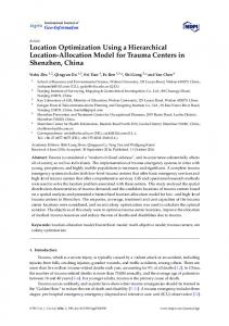
which is tractable. Note: though the emphasis has been on airframe design, a propulsion surrogate is also necessary for mission analysis. O BJECTIVE . Even with this improvement, there are many additional challenges that must be overcome. A computational framework is needed for integrating the aerostructural surrogate, propulsion surrogate, aerostructural analysis tool, mission analysis tool, and allocation models, which are all shown in Fig. 1. Many of these components have multiple instances—e.g., due to multiple missions—and some should be run in parallel, so the resulting complexity must be managed by automating parallel data passing between components. Another critical requirement is that gradients must be efficiently computed using the adjoint method to enable gradient-based optimization. All of these are requirements are addressed by using a recently-developed computational framework for large-scale optimization [8]. The objective of this paper is to perform simultaneous allocation-mission optimization with aerodynamic and propulsion surrogates. This problem represents a necessary intermediate step before solving the full design-missionallocation problem, and one that requires solutions to many of the key challenges for the full problem. 2 of 17 American Institute of Aeronautics and Astronautics
routes
trajectories
profit
Airline allocation
missions
mission constraints
fuel burn
Mission analysis
flight conditions
aerodynamic coefficients
Airframe surrogate
training points
training data
Airframe analysis
design constraints
propulsion variables
shape/sizing variables
Optimizer
throttle
engine output propulsion constraints
Propulsion surrogate
training points
training data
Propulsion analysis
Figure 1: Extended design structure matrix of the components necessary for simultaneous design-mission-allocation optimization.
The paper is organized as follows. First, we survey the aircraft allocation and mission optimization literatures in Sec. II. Next, we describe the methodology for the framework, the mission analysis, the allocation problem, and the combined problem in Sec. III. In Sec. IV, we describe the results for a suite of allocation-mission optimization problems.
II.
Literature survey
In this section, we survey the literatures in the aircraft allocation and mission optimization fields. In both areas, there are unique requirements introduced by our objective of combining allocation and mission optimization into one problem. On the allocation side, the key difference is that the problem is necessarily nonlinear and each evaluation of the objective and constraints is significantly more expensive. On the mission side, the main requirement is modularity because multiple mission instances are combined within a single allocation problem. A. Aircraft allocation One of the first applications of linear programming was the airline allocation problem, first published in 1956 [9], less than 10 years after the development of the simplex method in 1947 [10]. The original problem aimed to find the optimal allocation of aircraft to routes given uncertain demand [9], assuming a fixed cost incurred by flying a given route with a given type of aircraft. Beginning in 1966 [11], researchers began applying optimization to schedule design for flights, and later, the fleet assignment problem (FAP)—assigning aircraft to scheduled flights. In 1989, Abara showed that it is possible to use linear programming to solve FAPs of representative sizes [12]. Recent research has focused on improvements upon these formulations with for instance improved revenue models [13, 14], homogeneity of aircraft types at airports [15] or on legs [16], and simultaneous optimization of scheduling and fleet assignment [17]. More information can be found in survey articles by Clarke and Smith [18] and Barnhart et al. [19]. The fruits of research in this field have been used by airlines to improvement their operations and increase profit. For instance, algorithms for solving fleet assignment problems have been used by American Airlines [12], Delta Airlines [20], and US Airways [21]. For the current problem, the motivation for considering the allocation problem differs from that of the airlines. The objective is to solve the allocation problem as a tool to evaluate potential new aircraft designs by quantifying their airline-level benefits. It must be possible to simultaneously optimize the variables parametrizing the mission profile and aircraft design, so simplifying assumptions are used. Specifically, we use a variant of the original allocation
3 of 17 American Institute of Aeronautics and Astronautics
problem proposed in 1956 [9], and the considerations for scheduling are ignored. The current allocation formulation maximizes the profit across the entire network of the representative airline subject to the operational and demand constraints following the approach of [22, 23, 24, 25]. B. Mission optimization The prior art in mission profile optimization divides broadly into two categories, direct and indirect [26]. The direct approach first discretizes the equilibrium equations and applies the optimality conditions on the discretized equations. The indirect approach takes the reverse order—it first differentiates the equilibrium equations to derive continuous optimality conditions and then discretizes as the second step. Only the direct approach is reviewed as it is the one used in this chapter. Betts and Huffman performed trajectory optimization for a hypersonic re-entry vehicle using the direct approach [27]. They used a custom active-set gradient-based optimization algorithm with a sparse finite differencing method. Betts and Cramer applied a similar methodology to the trajectory optimization of commercial aircraft using sparse finite differencing and gradient-based optimization, and B-splines interpolants were used as the aerodynamic model [28]. Park and Clarke solved the trajectory optimization problem using the pseudospectral method, which discretizes state and control variables at points determined by a Gaussian quadrature [29]. An application of mission profile optimization is continuous descent approach (CDA), also known as optimized descent profile (ODP). ODP is one component of the next generation air transportation system (NextGen) currently being developed and implemented by the federal aviation administration (FAA). In addition to noise reductions, continuous descents yield fuel burn improvements compared to step descents. In the past decade, continuous and idle descent tests have been designed or implemented at Louisville [30], Denver [31], Los Angles [32], and Malta [33] international airports. Based on the current interest in ODP, the approach taken in this paper is to simultaneously optimize the mission profiles for each route while solving the allocation problem. The expected result is a rapid and smooth climb to a cruise-climb stage and then a continuous descent near idle, with the cruise altitudes determined by the optimizer. The numerical approach is similar to that of Betts and Cramer [28], with 2 key improvements. First, the derivatives needed for optimization are computed using the framework as opposed to finite differences for improved accuracy and efficiency. Second, the mission analysis is implemented in a modular way in the framework, facilitating integration with the allocation components, and in the future, with the aircraft design components.
III.
Methodology
A. Computational Modeling Framework T HEORY. The theoretical foundation for the computational framework is the representation of the multidisciplinary analysis (MDA) problem as a nonlinear system of equations [8]. A vector that solves this nonlinear system corresponds to the solution of the MDA problem and the process by which the MDA problem is solved can be interpreted as one of the known methods for solving a nonlinear system. The starting point for the theory is the concatenation of all design, state, intermediate, input, and output variables into a single vector of variables which is the vector of unknowns in the nonlinear system. This includes parameters and variables that are the outputs of the objective function and constraint functions. Each variable must have a residual function of the same size because for every scalar variable, there must be a corresponding equation that constrains its value. To achieve this, each variable is classified as an explicit, implicit, or independent variable. Let us assume there are n variables in total when all the variables are concatenated into one list. We also assume that each variable is itself a vector. For an explicit variable vi the residual is Ri = vi − Vi (v1 , . . . , vi−1 , vi+1 , . . . , vn ) = 0 where Vi is the function that computes vi , for an implicit variable the residual is simply Ri = Ri (v1 , . . . , vn ) = 0 since vi already has an associated residual function, Ri , and for an independent variable the residual is Ri = vi − vi∗ where vi∗ is the value at which we evaluate the computational model, since this is an input variable. If we define R = (R1 , . . . , Rn ) and u = (v1 , . . . , vn ), we can construct a nonlinear system R(u) = 0 as the mathematical representation of the MDA problem. Since the Jacobian ∂R/∂u is invertible in all practical problems, the inverse function theorem gives the following relationship for the Jacobian at a converged point [34]: ∂R T du T ∂R du =I= . ∂u dr ∂u dr
4 of 17 American Institute of Aeronautics and Astronautics
(3)
Equation (3) unifies all known discrete methods for computing derivatives with the left and right hand sides corresponding to the direct and adjoint methods, respectively, and the forward and reverse modes of algorithmic differentiation. The significance of Eq. (3) is that it allows the framework to automatically compute total derivatives simply by solving this linear system. The user is required to specify partial derivatives of all outputs with respect to all inputs for each discipline or block of code, and from this information, the framework can compute the total derivatives simply by solving the linear system in Eq. (3). Depending on whether the disciplines are coupled and have internal state variables and residuals, the process of solving this linear reduces to the adjoint method, chain rule, or one of many other known methods. I MPLEMENTATION The framework implementation has several functions. At its core, it is a piece of software that allows the user to define the components or disciplines of the problem in a modular way. The framework automates transfer of data between components, including parallel data communication when the source and destination of the data are on different processors, and provides the infrastructure for solving the nonlinear system and Eq. (3). The framework uses object-oriented programming, with instances of a System class as the basic building blocks. In general, the nonlinear system R(u) = 0 is hierarchically decomposed, where the top-level system owns the full set of variables u and the set of variables is partitioned at each subsequent level. Figure 2 shows the hierarchy tree that results from this decomposition in which systems contain other systems and each system is uniquely defined by the set of variables it contains.
S00 S02 S04 S05
S06
S10 S03
S07
S11
S12 S13
S13
Figure 2: Hierarchy tree for a notional problem. The circles are variables and the rounded rectangles are systems with those in green considered the leaves of the tree (if the circle nodes are ignored). Each system is responsible for implementing methods that evaluate its owned entries of the R vector and the ∂R ∂u matrix. Each system can then solve its child systems using nonlinear or linear block Gauss-Seidel or Jacobi, and the child systems may contain their own child systems or solve their variables using a monolithic approach such as Newton’s method. Systems can also optionally implement an approximate inverse for its Jacobian if a preconditioner is available. Both the Jacobian and the preconditioner are implemented as linear operators so the framework does not make restrictions on whether they are sparse or dense or have some other special structure, or if only the matrixvector product operation is available. The framework uses the Portable, Extensible Toolkit for Scientific Computation (PETSc) [35] to handle parallel data communication among systems, and for PETSc’s built-in iterative solvers. For more details, we refer the reader to Hwang and Martins [8]. B. The mission problem The main components of the mission analysis are formed by the equilibrium equations for the aircraft and the ordinary differential equation (ODE) for fuel weight. For the former, the vertical equilibrium determines the required angle of attack to roughly match lift with weight, the horizontal equilibrium determines the engine throttle setting to roughly match thrust with drag, and the moment equilibrium determines the elevator deflection to trim the aircraft. The
5 of 17 American Institute of Aeronautics and Astronautics
equations are L + W cos γ − T sin α +
W 2 dγ v cos γ =0 g dx
W dv v cos γ =0 g dx � 2 � d γ dγ dv 2 2 (v cos γ) M −I + v(cos γ) = 0, dx2 dx dx T cos α + D + W sin γ +
(4) (5) (6)
where α is the angle of attack and γ is the climb or descent angle. Assuming quasi-steady flight conditions, the terms containing derivatives with respect to x can be ignored. Dropping these terms and expressing in terms of non-dimensional coefficients yields 1 1 2 ˜ ρv S CL + W cos γ − ρv 2 S C˜T sin α = 0 2 2 1 2 ˜ 1 ρv S CT cos α + ρv 2 SCD + W sin γ = 0 2 2 C˜M = 0.
(7) (8) (9)
The system of equations is completed by adding surrogate models for the aerodynamics and propulsion, which are of the form C˜L − CL (h, M, α, η) = 0 (10) C˜M − CM (h, M, α, η) = 0 C˜T − CT (h, M, t) = 0,
(11) (12)
where the variables with tildes indicate target variables while CL , CD , CM , and CT are functions representing the aerodynamic or propulsion surrogates. In this problem, the aerodynamic surrogates are tensor-product B-splines interpolants, and the propulsion surrogate is a simple linear function. The fuel weight is computed by solving the ODE, {SF C} 21 ρv 2 SCT , W˙ f = v cos γ
(13)
where SF C is the thrust-specific fuel consumption, and CT is the thrust coefficient. This problem involves multiple disciplines that are coupled. The rate of fuel burn at a given point during the flight depends on the engine output, which is determined by the amount of aerodynamic drag that the engines must overcome. However, the amount of drag depends on how much lift must be produced to counteract the weight of the aircraft, which in turn is affected by the total amount of fuel required, completing the feedback loop. Figure 3 shows a class diagram containing the components and solvers used in the computational model. The toplevel System object, Mission, contains five systems that have no feedback, so nonlinear and linear block Gauss–Seidel converge in one iteration. One of the five subsystems, Coupled analysis, contains the aforementioned feedback loop involving fuel burn, thrust, drag, lift, and weight. For this system, Newton’s method is used to solve the nonlinear system with a few iterations of nonlinear block Gauss–Seidel used as a start-up strategy, the linear systems that arise are solved using fGMRES, and the preconditioner is a few iterations of linear block Gauss–Seidel. Coupled analysis, in turn, contains a system that defines implicit state variables, so it also uses a Newton–Krylov solver. The mission-only optimization is a nonlinear programming (NLP) problem with the objective of minimizing fuel burn and is stated below (NLP-m). The design variables are the B-spline control points of the parametrized altitude profile with ncp B-spline control points and npt discretization points. In this paper, we use ncp = 50 and npt = 250. The initial and final altitudes are constrained to be zero, and slope constraints are imposed on the altitude profile with a value of 35◦ for both climbing and descending. The throttle setting is constrained to be between idle (10%) and full (100%). The slope constraints are linearly mapped from the design variables, but the throttle setting is a nonlinear function of the design variables and state variables, so its derivatives are computed using the adjoint method. Since it is costly to solve one adjoint for each of the npt points, the throttle constraints are aggregated using Kreisselmeier– Steinhauser functions [36] to reduce to a single idle-throttle constraint and a single full-throttle constraint.
6 of 17 American Institute of Aeronautics and Astronautics
Legend CompoundSystem IndependentSystem ImplicitSystem ExplicitSystem
Symbols W aircraft weight L lift D drag T thrust
Mission Nonlin: GS Linear: GS Precon: N/A
Inputs
Flight conditions
B-splines
Outputs
Coupled analysis Nonlin: Newton Linear: Krylov Precon: GS
Vert. equilibrium
Aerodynamics
Hor. equilibrium
Propulsion
Fuel weight
D→T
˙ T →W
˙ →W W
Nonlin: Newton Linear: Krylov Precon: None W →L
L→D
Figure 3: A class diagram showing the System instances in the aircraft mission problem.
minimize fuel burn with respect to altitudek ∈ [0, max altitude] , 1 ≤ k ≤ ncp subject to altitude1 = 0 altitudencp = 0 idle throttle ≤ throttle (KS) throttle ≤ max throttle (KS) min slope ≤ slopek ≤ max slope , 1 ≤ k ≤ npt
(NLP-m)
C. The allocation problem The allocation problem mimics the motivation of a profit-seeking airline. Given nrt routes and nac types of aircraft, the allocation problem we wish to solve in this paper seeks to maximize profit by optimally allocating the available aircraft to the routes with constraints on the number of each aircraft type available as well as the demand for each. There are 3 equations relevant to this problem. In this paper, i is used to index routes, and j is used to index types of aircraft. The design variables are pax flti,j , which is the number of passenger per flight, and flt dayi,j , which is the number of flights per day. Both design variables are arrays over routes and types of aircraft. The first is profit, which is given by profit =
nrt X nac X � i
−
j
nrt X nac X � i
j
price paxi,j · pax flti,j · flt dayi,j
�
(14)
� (cost flti,j + cost fuel · fuel flti,j ) · flt dayi,j ,
(15)
where price paxi,j is the ticket price per flight, cost flti,j is the total cost of operating a flight minus fuel, cost fuel is the cost per unit fuel, and fuel flt is the total fuel burn on a flight. In some cases, fuel flti,j is assumed to be a constant during an allocation optimization, and in others, it is the output of the mission analysis. The second equation is an inequality that enforces that the total number of passengers flown on a route is less than the demand on that route, and it is given by total paxi =
nac X � � pax flti,j · flt dati,j ≤ demandi , j
1 ≤ i ≤ nrt ,
(16)
where demandi is the total number of passengers who are looking to fly on a given route. This inequality is enforced for each route i.
7 of 17 American Institute of Aeronautics and Astronautics
The final equation is another inequality that constrains aircraft operation time based on the total number of available aircraft for a given type, and it is given by total usagej =
nrt X � i
� flt dayi,j · (time flti,j (1 + maintj ) + turn flt) ≤ 12hr · num acj ,
1 ≤ j ≤ nac ,
(17)
where time flti,j is the block time for a flight, maintj is the maintenance time required as a multiple of block time, turn flt is the turnaround time between flights, and num acj is the number of aircraft available for a given type. As with block fuel, block time is either a constant during optimization, or it is computed by the mission analysis. This inequality is enforced for each aircraft type j. The allocation-only optimization problem is a mixed-integer linear programming (MILP) problem and is stated below (MILP-a). In this case, block fuel and block time are constants, and they are not dynamically re-computed during optimization by running mission analysis. The objective function is profit, and the two integer design variables are passengers per flight and flights per day for each route and type of aircraft. Demand constraints are enforced for each route, and aircraft availability constraints are enforced for each type of aircraft. Here, the demand is assumed symmetric and the model assumes that each aircraft type makes a round trip on each route. This partially addresses the scheduling-related constraints. maximize profit with respect to pax flti,j ∈ [0, ac capacityj ] ∩ N , 1 ≤ i ≤ nrt , 1 ≤ j ≤ nac 1 ≤ i ≤ nrt , 1 ≤ j ≤ nac flt dayi,j ∈ [0, ∞) ∩ N , subject to total paxi ≤ demandi , 1 ≤ i ≤ nrt total usagej ≤ num acj , 1 ≤ j ≤ nac
(MILP-a)
D. The allocation-mission problem The main optimization problem we wish to solve in this paper is the simultaneous allocation-mission optimization with profit as the objective function. This top-level problem includes the allocation problem as well as the mission problems for each route and each type of aircraft. However, for this paper, mission analyses are only run for only the new types of aircraft. The rationale is that in future work with the simultaneous design-mission-allocation optimization, the existing types of aircraft have fixed designs so the block fuel and block time only depend on the routes, which are fixed, and the weight of the passengers, which does not have a large influence. In contrast, the new types of aircraft would be simultaneously designed during the design-mission-allocation optimization, so it is necessary to re-compute the mission analyses dynamically during optimization. In light of this, let us call the number of new types of aircraft nnac . The simultaneous allocation-mission optimization is a mixed-integer nonlinear programming (MINLP) problem and is stated below (MINLP-a-m). To lower the difficulty of the problem, the number of passengers per flight can be relaxed as a continuous variable; however, the same assumption cannot be made for the number of flights per day because the small values signify that relaxing the integer constraints would significantly change the optimization problem.
maximize profit with respect to pax flti,j ∈ [0, ac capacityj ] , flt dayi,j ∈ [0, ∞) ∩ N , altitudei,j,k ∈ [0, max altitude] ,
1 ≤ i ≤ nrt , 1 ≤ j ≤ nac 1 ≤ i ≤ nrt , 1 ≤ j ≤ nac 1 ≤ i ≤ nrt , 1 ≤ j ≤ nnac 1 ≤ k ≤ ncp subject to total paxi ≤ demandi , 1 ≤ i ≤ nrt total usagej ≤ num acj , 1 ≤ j ≤ nac altitudei,j,1 = 0 , 1 ≤ i ≤ nrt , 1 ≤ j ≤ nnac altitudei,j,ncp = 0 , 1 ≤ i ≤ nrt , 1 ≤ j ≤ nnac idle throttle ≤ throttlei,j (KS) , 1 ≤ i ≤ nrt , 1 ≤ j ≤ nnac throttlei,j ≤ max throttle (KS) , 1 ≤ i ≤ nrt , 1 ≤ j ≤ nnac min slope ≤ slopei,j,k ≤ max slope , 1 ≤ i ≤ nrt , 1 ≤ j ≤ nnac 1 ≤ k ≤ npt
8 of 17 American Institute of Aeronautics and Astronautics
(MINLP-a-m)
The MINLP problem is solved using the branch-and-bound method [37] to formulate a series of continuous NLP problems that eventually generate an integer solution, and the continuous problem is shown below (NLP-a-m). The continuous NLP problems are solved using SNOPT [38], using a modified version of the pyOpt interface [39]. SNOPT is a gradient-based optimizer that implements the sequential quadratic programming (SQP) method, and it is specifically designed for nonlinear constrained optimization problems that are large-scale and sparse.
maximize profit with respect to pax flti,j ∈ [0, ac capacityj ] , flt dayi,j ∈ [0, ∞) , altitudei,j,k ∈ [0, max altitude] ,
1 ≤ i ≤ nrt , 1 ≤ j ≤ nac 1 ≤ i ≤ nrt , 1 ≤ j ≤ nac 1 ≤ i ≤ nrt , 1 ≤ j ≤ nnac 1 ≤ k ≤ ncp subject to total paxi ≤ demandi , 1 ≤ i ≤ nrt 1 ≤ j ≤ nac total usagej ≤ num acj , altitudei,j,1 = 0 , 1 ≤ i ≤ nrt , 1 ≤ j ≤ nnac altitudei,j,ncp = 0 , 1 ≤ i ≤ nrt , 1 ≤ j ≤ nnac 1 ≤ i ≤ nrt , 1 ≤ j ≤ nnac idle throttle ≤ throttlei,j (KS) , throttlei,j ≤ max throttle (KS) , 1 ≤ i ≤ nrt , 1 ≤ j ≤ nnac min slope ≤ slopei,j,k ≤ max slope , 1 ≤ i ≤ nrt , 1 ≤ j ≤ nnac 1 ≤ k ≤ npt
(NLP-a-m)
The overall algorithm that solves (MINLP-a-m) is described in Algorithm 1. The first step is to solve (NLP-m) for each route and each aircraft type using SNOPT in order to determine the block times and block fuels to be used in the next step. We use the linprog function in SciPy’s optimize package via NASA’s OpenMDAO framework [40] to solve (MILP-a) to generate a good initial solution for the branch-and-bound algorithm. Next, we begin the branchand-bound phase by initializing the tree and adding the first node, which is (NLP-a-m) that uses the initial values for the allocation design variables from the solution to (MILP-a) and the initial values for the mission design variables from the solution to (NLP-m) for each mission. The remainder of the algorithm implements the depth-first branchand-bound algorithm. An important characteristic of this algorithm is that when branching for a variable xk , all of the initial values from the parent node are used, except for xk itself, which is taken to be the same as the upper or lower bound. This allows (NLP-a-m) to be solved in one or a very small number of NLP iterations in many cases, yielding improved efficiency. Algorithm 1 Solution of the allocation-mission optimization problem, (MINLP-a-m) 1: 2: 3: 4: 5: 6: 7: 8: 9: 10: 11: 12: 13: 14: 15: 16: 17: 18: 19: 20: 21:
for i ← 1, nrt do for j ← 1, nac do Solve (NLP-m) to determine block fuel and time for the (i, j)th mission end for end for Solve (MILP-a) Create the branch and bound tree Add the first node for an (NLP-a-m) starting from (MILP-a) and (NLP-m) solutions while Nodes exist do Solve (NLP-a-m) in the deepest node (depth-first strategy) if Solution is better than the best integer solution then if Solution is integer then Store solution—this is the new solution else k ← index of integer variable furthest from an integer Add a node for an (NLP-a-m) with upper bound and initial value of xk changed to f loor(xk ) Add a node for an (NLP-a-m) with lower bound and initial value of xk changed to ceiling(xk ) end if end if Delete current node end while
9 of 17 American Institute of Aeronautics and Astronautics
IV.
Results
This section presents a suite of allocation-mission optimization results obtained using Algorithm 1. We start by describing the routes and the types of aircraft in the problem we solved, and present 4 results. First, we show the predicted increase in profit for an airline if it purchases new aircraft instead of existing aircraft. Second, we show that there is a difference between the results of allocation-only optimization (MILP-a) and allocation-mission optimization (MINLP-a-m). Next, we explore the presence of local optima in (NLP-a-m) and show that (MINLP-a-m) is highly sensitive to the starting point. Finally, we discuss the numerical performance of the allocation-mission analysis and optimization algorithm. A. The problem The results in this paper solve a 3-route problem with ranges of roughly 7000 nmi, 5500 nmi, and 2500 nmi. The routes have been chosen to represent a network with a hub in Newark, New Jersey and the following destinations: Hong Kong; Kuwait City, Kuwait; and Quito, Ecuador. The routes are summarized in Tab. 1 and shown graphically in Fig. 4. Route Range [nmi] Demand
Newark, New Jersey (EWR) Hong Kong (HKG) 6998 1200
Newark, New Jersey (EWR) Kuwait City, Kuwait (KWI) 5546 550
Newark, New Jersey (EWR) Quito, Ecuador (IQT) 2509 700
Table 1: The 3 routes considered in the allocation-mission optimization .
Figure 4: Map of the cities and the routes (generated using the Great Circle Mapper: www.gcmap.com). Newark, New Jersey is chosen as the hub. We consider 6 aircraft types, 4 existing ones and 2 hypothetical next-generation aircraft. The Boeing 737-800 (B737), Boeing 777-200ER (B777), Boeing 747 (B747), and Boeing 787 (B787) have been chosen as the existing aircraft to cover a variety of design ranges and seating capacities. The two new aircraft are a notional advanced conventional design based on the Common Research Model [41] and a blended wing body concept based on Liebeck [42] with a reduced seating capacity. The aircraft types are summarized in Tab. 2 with seating capacities shown after applying an 80 % load factor. Table 2 also shows the 4 allocation-mission optimization problems we solved, representing
10 of 17 American Institute of Aeronautics and Astronautics
Aircraft Category Capacity Scenario S-base S-CRM S-BWB S-both
Boeing 737-800 Existing 122
Boeing 777-200ER Existing 207
Boeing 747-400 Existing 294
Boeing 787-8 Existing 200
20 20 20 20
24 24 24 20
24 24 24 20
8
CRM: advanced conventional New 300
BWB: blended wing body New 400
8 8
8 8
Table 2: The types of aircraft considered in the allocation-mission optimization. The bottom four lines show the number of each aircraft type available in each of the four scenarios.
different scenarios in which the hypothetical airline chooses to buy different aircraft. The cost, ticket price and the performance data of the existing aircraft for the different routes in the network are obtained using the simulation tool FLEET [24, 25]. For the new aircraft, the ticket price, no-fuel direct operating cost and the indirect operating cost are also obtained from an equivalent aircraft modeled in FLEET. The current model do not account for airline competition and assumes the ticket prices are fixed across types of aircraft on a given route. B. Profit increase with new aircraft Figure 5 shows the profit after optimization for each of the 4 scenarios. The results agree with intuition because the CRM and BWB both represent an improvement over the existing aircraft. The CRM design is based on the B777, but it is assumed to have a larger seating capacity and higher aerodynamic efficiency since it is a next generation aircraft. The B787 has the range of the CRM but a lower seating capacity, while the B747 has the seating capacity but a lower range and lower efficiency as it is a much older design. Thus, the S-CRM scenario provides a 192 % improvement in profit over the baseline S-base, the S-BWB scenario provides a 323 % due to its larger seating capacity, and the S-both scenario provides a further improvement with 414 % compared to the baseline.
+414% +323%
Profit [$ × 106 ]
3
2
+192%
1
0 S-base
S-CRM S-BWB
S-both
Figure 5: Comparison of profit for the four scenarios at the solution to (MINLP-a-m). The results show an increase in profit when the hypothetic airline purchases the next-generation aircraft.
C. Allocation versus allocation-mission optimization Figure 6 compares the optimized profit among 4 cases: (MINLP-a-m) without the (MILP-a) initialization, (MILP-a), (MINLP-a-m), and (NLP-a-m). This subsection focuses on (MILP-a) versus (MINLP-a-m)—i.e. allocation-only 11 of 17 American Institute of Aeronautics and Astronautics
optimization versus allocation-mission optimization. We see a small increase in profit in all three scenarios with the allocation-mission optimization because it more accurately computes the block fuel and block time for the new aircraft. In particular, the block fuel values used in (MILP-a) assume the aircraft always fly at full capacity—thus, (MILP-a) likely underpredicts profit because the actual fuel burn is lower when the aircraft flies with fewer passengers than its seating capacity. However, this is a minor difference, and we remind the reader that the true motivation for incorporating mission analysis in the allocation problem is to enable design-mission-allocation optimization, and this paper develops many of the methods needed for optimization with all three simultaneously considered.
+0.1% +14.5%
Profit [$ × 106 ]
3
2
+12.8%
1
0 S-CRM
S-BWB
MINLP-a-m (local opt.) MINLP-a-m (solution)
S-both MILP-a (alloc. only) NLP-a-m (relaxed)
Figure 6: Comparison of optimized profits. The colors represent, in order: (MINLP-a-m) not initialized to the solution to (MILP-a) (orange), (MILP-a) (red), (MINLP-a-m) initialized to the solution to (MILP-a) (blue), and (NLP-a-m) solved in the first node of the branch-and-bound algorithm. The results show clear local minima and an increase in profit in the allocation-mission optimization compared to the allocation-only optimization.
D. Local optima One significant concern when incorporating mission analysis into the allocation problem is that the problem becomes nonlinear, so there is potential for local optima that represent significantly worse profit than the global optimum. Figure 6 shows that there is indeed a large difference between two solutions to (MINLP-a-m): one in which Algorithm 1 is run as is and one in which Algorithm 1 is run without the (MILP-a) initialization (line 6). In Fig. 6, the orange bars are several times smaller than the blue bars for each scenario. Figure 7 confirms that the integer design variables—flights per day—consistently show large changes between the two optima. These results highlight two aspects to the importance of the (MILP-a) initialization step (line 6) in Algorithm 1. First, it is not possible to guarantee convergence to a global minimum in nonlinear optimization problems that do not satisfy any convexity conditions, but Algorithm 1 provides a reasonably good local optimum by starting from the global optimum of the linear problem, (MILP-a). The initial (NLP-a-m) and the branch-and-bound method then guarantee that the solution to which it converges is no worse than the initial point provided by the linear optimization. The second benefit is the tremendous efficiency afforded by this two-step approach. The linear optimization (MILP-a) is inexpensive, so it quickly gets close to the solution of the nonlinear optimization (MINLP-a-m), after which branch-and-bound begins from a good starting point. Fig. 8 shows that the continuous solution of the initial (NLP-a-m) solved in the first node of the branch-and-bound is not significantly different from the solution of (MILP-a), and the solution of (MINLP-a-m) is in turn very similar as well. In fact, the branch-and-bound only forces the integer variables to one of the nearest integers, suggesting that the (NLP-a-m) problem is locally convex in a large enough area containing the nearby integers, but multimodal over a larger region since at least one other local optimum was
12 of 17 American Institute of Aeronautics and Astronautics
5
Flights per day
S-CRM S-BWB S-both
S-CRM (local) S-BWB (local) S-both (local)
4 3 2 1 0 B737 7.0
5.5
B777 2.5
7.0
5.5
B747 2.5
7.0 5.5 2.5 Range[nm ×103 ]
CRM 7.0
5.5
BWB 2.5
7.0
5.5
2.5
Figure 7: Optimal values of the (round trip) flights per day design variable comparing (MINLP-a-m) with and without (local) initialization to the solution to (MILP-a). The results show two distinct local minima in (MINLP-a-m).
found. S-CRM (MILP-a) S-BWB (MILP-a) S-Both (MILP-a)
5
Flights per day
4
S-CRM (NLP-a-m) S-BWB (NLP-a-m) S-Both (NLP-a-m)
S-CRM (MINLP-a-m) S-BWB (MINLP-a-m) S-Both (MINLP-a-m)
3 2 1 0 B737 7.0
5.5
B777 2.5
7.0
5.5
B747 2.5
7.0 5.5 2.5 Range[nm ×103 ]
CRM 7.0
5.5
BWB 2.5
7.0
5.5
2.5
Figure 8: Optimal values of the (round trip) flights per day design variable comparing the allocation-only solution (MILP-a), the relaxed allocation-mission solution (NLP-a-m), and the integer allocation-mission solution (MINLP-a-m). The results show that the relaxed simultaneous solution is close to the allocation-only solution and the integer simultaneous solution is close to the relaxed simultaneous solution. This observation is significant from a computational standpoint because the branch-and-bound method converges in a small number of iterations. For this 3-route problem, all cases converged in 5-20 node evaluations, and initial studies of 5-route problems show the same results. Furthermore, many of the (NLP-a-m) problems solved during branch-and-bound converge in one iteration or a small number of iterations because the initial point is often the solution. E. Numerical performance Figure 9 shows the scaling of an analysis for the (NLP-a-m) formulation and an adjoint solution. It shows the execution time for problems with between 1 and 16 routes. The scaling is between linear and quadratic, but in future studies, the mission analyses can be easily parallelized since there is no coupling between mission analyses for different routes and aircraft. Figure 10 shows the convergence history for the solution of (NLP-a-m) with 3 routes and 2 new aircraft, resulting in 330 design variables in total. The fact that we can achieve such a high level of convergence provides confidence that the derivatives are computed accurately and the design variables and constraints are properly scaled. Table 3 shows
13 of 17 American Institute of Aeronautics and Astronautics
Execution time (s)
Evaluation
101
100 Derivatives 10−1 103.8
104 104.2 104.4 104.6 Number of unknowns
104.8
Figure 9: Execution time versus number of total unknowns in the simulation for an analysis and an adjoint solution with problems ranging from 1 route to 16 routes. The scaling is between linear and quadratic.
the times for solving (MINLP-a-m) for the various cases.
V.
Conclusion
Merit function
10
200
2 Feasibility
−3
10−5
Merit function
Convergence metric
10−1
Optimality 0
150 1
100
# superbasic vars.
50 0
20 Function evaluations
40
# superbasic variables
In this paper, we developed an algorithm for performing simultaneous allocation-mission optimization. This required four components: the use of a computational framework for automatically solving the coupled simulation and computing derivatives using the adjoint method, an efficient mission analysis algorithm that uses surrogates for aerodynamics and propulsion, implementation of the allocation problem within the framework that couples an arbitrary number of mission analyses together, and a method for solving the mixed-integer allocation-mission optimization problem. The key step in this method is the initialization of the branch-and-bound allocation-mission optimization using the solution of the allocation-only optimization. We applied this algorithm to the allocation of 4 existing aircraft and 2 next-generation aircraft to a 3-route network and presented three conclusions. First, the algorithm found significant profit increases if the airline chooses to purchase the next-generation aircraft. Compared to a baseline, purchasing 8 advanced conventional aircraft yielded a 192 % increase in profit, purchasing 8
0 0
25 Function evaluations
50
Figure 10: Optimization convergence history for a 3-route, 2-new aircraft problem with 330 design variables. The tight convergence of optimality and feasibility helps verify the accuracy of the derivative computation.
14 of 17 American Institute of Aeronautics and Astronautics
Case S-CRM (local) S-CRM S-BWB (local) S-BWB S-both (local) S-both
Time [min.] 7.7 20.4 9.0 20.5 33.3 40.6
Table 3: The execution times for the solution of (MINLP-a-m).
blended wing body aircraft yielded a 323 % increase in profit, and purchasing 8 of each yielded a 414 % increase in profit with the optimal allocation. Second, the allocation-mission optimization produced a higher profit than allocation-only optimization. Part of the difference is attributed to the fact that block fuel is computed dynamically during optimization using the allocated number of passengers, rather than pre-computing block fuel assuming full capacity. However, this error is minor, and the true benefit of simultaneously considering mission during the allocation problem is that this enables also incorporating design in the simultaneous optimization in future work. Third, we found multiple local optima in the mixed-integer allocation-mission problem, and they yielded profit numbers that are 2-3 times apart. However, we showed that our algorithm efficiently finds a good local optimum by using an allocation-only optimization to find a good starting point. This is advantageous because linear programming has a low computational cost and it finds the global optimum. In practice, the solution to the first relaxed allocationmission optimization during branch-and-bound deviates a small amount from the linear solution and the branch-andbound method, in turn, finds one of the neighboring integer points as the solution. The significance of this is that many nodes in the branch-and-bound algorithm converge very quickly during the continuous optimization. The significance of this work is the demonstration of an efficient algorithm for solving simultaneous allocationmission optimization problems that uses an approach that naturally extends to design-mission-allocation optimization. Therefore, the next step in this research effort is adding design to the simultaneous optimization problem. As part of this step, an important avenue for future work is testing the current algorithm with the mission analyses parallelized for improved scalability.
VI.
Acknowledgments
This work was supported by NASA through grant number NNX14AC73A. The authors would like to thank Justin S. Gray from the NASA Glenn Research Center for his help implementing the linear allocation problem in OpenMDAO and Rhea P. Liem from the University of Toronto for providing the aerodynamic surrogate models for the CRM and BWB.
15 of 17 American Institute of Aeronautics and Astronautics
References [1] Rutherford, D. and Zeinali, M., “Efficiency Trends for New Commercial Jet Aircraft 1960 to 2008,” The International Council on Clean Transportation, 2009. [2] ICAO Secretariat, “Aircraft technology improvements,” ICAO Environmental Report 2010, International Civil Aviation Organization, 2010. [3] Kennedy, G. J. and Martins, J. R. R. A., “A Comparison of Metallic and Composite Aircraft Wings Using Aerostructural Design Optimization,” 14th AIAA/ISSMO Multidisciplinary Analysis and Optimization Conference, Indianapolis, IN, Sep. 2012, AIAA-2012-5475. [4] Kennedy, G. J., Kenway, G. K., and Martins, J. R. R. A., “A Comparison of Metallic, Composite and Nanocomposite Optimal Transonic Transport Wings,” Tech. rep., NASA, March 2014, CR-2014-218185. [5] Lyu, Z. and Martins, J. R. R. A., “Aerodynamic Design Optimization Studies of a Blended-Wing-Body Aircraft,” Journal of Aircraft, Vol. 51, No. 5, September 2014, pp. 1604–1617. doi:10.2514/1.C032491. [6] Kenway, G. K. W. and Martins, J. R. R. A., “Multipoint High-Fidelity Aerostructural Optimization of a Transport Aircraft Configuration,” Journal of Aircraft, Vol. 51, No. 1, January 2014, pp. 144–160. doi:10.2514/1.C032150. [7] Liem, R. P., Kenway, G. K., and Martins, J. R. R. A., “Multi-point, multi-mission, high-fidelity aerostructural optimization of a long-range aircraft configuration,” Proceedings of the 14th AIAA/ISSMO Multidisciplinary Analysis and Optimization Conference, Indianapolis, IN, Sept. 2012. doi:10.2514/6.2012-5706, (Best Paper Award). [8] Hwang, J. T. and Martins, J. R. R. A., “A parallel hierarchical algorithmic framework for large-scale simulation and optimization,” University of Michigan, 2015. [9] Ferguson, A. R. and Dantzig, G. B., “The allocation of aircraft to routes-an example of linear programming under uncertain demand,” Management science, Vol. 3, No. 1, 1956, pp. 45–73. [10] Gass, S., “George B. Dantzig,” Profiles in Operations Research, edited by A. A. Assad and S. I. Gass, Vol. 147 of International Series in Operations Research & Management Science, Springer US, 2011, pp. 217–240. doi:10.1007/978-1-4419-6281-2 13. [11] Simpson, R. W., “Computerized schedule construction for an airline transportation system,” Department of Aeronautics and Astronautics, Massachusetts Institute of Technology, Vol. 232, 1966. [12] Abara, J., “Applying integer linear programming to the fleet assignment problem,” Interfaces, Vol. 19, No. 4, 1989, pp. 20–28. [13] Barnhart, C., Farahat, A., and Lohatepanont, M., “Airline fleet assignment with enhanced revenue modeling,” Operations research, Vol. 57, No. 1, 2009, pp. 231–244. [14] Dumas, J., Aithnard, F., and Soumis, F., “Improving the objective function of the fleet assignment problem,” Transportation Research Part B: Methodological, Vol. 43, No. 4, 2009, pp. 466–475. [15] Johnson, E. L., “Robust airline fleet assignment: imposing station purity using station decomposition,” Algorithmic Applications in Management, Springer, 2005, pp. 1–2. [16] B´elanger, N., Desaulniers, G., Soumis, F., Desrosiers, J., and Lavigne, J., “Weekly airline fleet assignment with homogeneity,” Transportation Research Part B: Methodological, Vol. 40, No. 4, 2006, pp. 306–318. [17] Lohatepanont, M. and Barnhart, C., “Airline schedule planning: Integrated models and algorithms for schedule design and fleet assignment,” Transportation Science, Vol. 38, No. 1, 2004, pp. 19–32. [18] Clarke, M. and Smith, B., “Impact of operations research on the evolution of the airline industry,” Journal of Aircraft, Vol. 41, No. 1, 2004, pp. 62–72. [19] Barnhart, C., Belobaba, P., and Odoni, A. R., “Applications of operations research in the air transport industry,” Transportation science, Vol. 37, No. 4, 2003, pp. 368–391. [20] Subramanian, R., Scheff, R. P., Quillinan, J. D., Wiper, D. S., and Marsten, R. E., “Coldstart: fleet assignment at delta air lines,” Interfaces, Vol. 24, No. 1, 1994, pp. 104–120. [21] Kontogiorgis, S. and Acharya, S., “US Airways automates its weekend fleet assignment,” Interfaces, Vol. 29, No. 3, 1999, pp. 52–62. [22] Zhao, J., Tetzloff, I. J., Tyagi, A., Dikshit, P., Mane, M., Agusdinata, D., Crossley, W. A., and DeLaurentis, D., “Assessing New Aircraft and Technology Impacts on Fleet-Wide Environmental Metrics including Future Scenarios,” 48th AIAA Aerospace Sciences Meeting Including the New Horizons Forum and Aerospace Exposition, Orlando, Florida, 2010. [23] Mane, M., Tetzloff, I., Zhao, J., Noth, K., Agusdinata, D., DeLaurentis, D., and Crossley, W., “Fleet-wide environmental impact of future aircraft technologies,” 10th AIAA Aviation Technology, Integration, and Operations Conference (ATIO), 2010. [24] Crossley, W. and DeLaurentis, D., “System-of-systems approach for assessing new technologies in NGATS,” Purdue University, 2007.
16 of 17 American Institute of Aeronautics and Astronautics
[25] Govindaraju, P. and Crossley, W. A., “Profit Motivated Airline Fleet Allocation and Concurrent Aircraft Design for Multiple Airlines,” Aviation Technology, Integration, and Operations Conference, Aug 2013, AIAA 2013-4391. [26] Betts, J. T., “Survey of numerical methods for trajectory optimization,” Journal of guidance, control, and dynamics, Vol. 21, No. 2, 1998, pp. 193–207. [27] Betts, J. T. and Huffman, W. P., “Application of sparse nonlinear programming to trajectory optimization,” Journal of Guidance, Control, and Dynamics, Vol. 15, No. 1, 1992, pp. 198–206. [28] Betts, J. T. and Cramer, E. J., “Application of direct transcription to commercial aircraft trajectory optimization,” Journal of Guidance, Control, and Dynamics, Vol. 18, No. 1, 1995, pp. 151–159. [29] Park, S. G. and Clarke, J.-P., “Vertical Trajectory Optimization for Continuous Descent Arrival Procedure,” AIAA Guidance, Navigation, and Control Conference, Minneapolis (Minnesota-USA), Paper, Vol. 4757, 2012, p. 2012. [30] Clarke, J.-P. B., Ho, N. T., Ren, L., Brown, J. A., Elmer, K. R., Zou, K., Hunting, C., McGregor, D. L., Shivashankara, B. N., Tong, K.-O., et al., “Continuous descent approach: Design and flight test for Louisville International Airport,” Journal of Aircraft, Vol. 41, No. 5, 2004, pp. 1054–1066. [31] Shresta, S., Neskovic, D., and Williams, S., “Analysis of continuous descent benefits and impacts during daytime operations,” 8th USA/Europe Air Traffic Management Research and Development Seminar (ATM2009), Napa, CA, 2009. [32] Clarke, J.-P., Brooks, J., Nagle, G., Scacchioli, A., White, W., and Liu, S., “Optimized Profile Descent Arrivals at Los Angeles International Airport,” Journal of Aircraft, Vol. 50, No. 2, 2013, pp. 360–369. [33] Micallef, M., Chircop, K., Zammit-Mangion, D., and Sammut, A., “Revised approach procedures to support optimal descents into Malta International Airport,” CEAS Aeronautical Journal, 2014, pp. 1–15. [34] Martins, J. R. R. A. and Hwang, J. T., “Review and Unification of Methods for Computing Derivatives of Multidisciplinary Computational Models,” AIAA Journal, Vol. 51, No. 11, November 2013, pp. 2582–2599. doi:10.2514/1.J052184. [35] Balay, S., Gropp, W. D., McInnes, L. C., and Smith, B. F., “Efficient Management of Parallelism in Object Oriented Numerical Software Libraries,” Modern Software Tools in Scientific Computing, edited by E. Arge, A. M. Bruaset, and H. P. Langtangen, Birkh¨auser Press, 1997, pp. 163–202. [36] Kreisselmeier, G. and Steinhauser, R., “Systematic Control Design by Optimizing a Vector Performance Index,” International Federation of Active Controls Syposium on Computer-Aided Design of Control Systems, Zurich, Switzerland, 1979. [37] Bertsimas, D. and Tsitsiklis, J. N., “Introduction to linear optimization,” 1997. [38] Gill, P. E., Murray, W., and Saunders, M. A., “SNOPT: An SQP algorithm for large-scale constrained optimization,” SIAM Journal of Optimization, Vol. 12, No. 4, 2002, pp. 979–1006. doi:10.1137/S1052623499350013. [39] Perez, R. E., Jansen, P. W., and Martins, J. R. R. A., “pyOpt: a Python-Based Object-Oriented Framework for Nonlinear Constrained Optimization,” Structural and Multidisciplinary Optimization, Vol. 45, No. 1, January 2012, pp. 101–118. doi:10.1007/s00158-011-0666-3. [40] Gray, J., Moore, K. T., Hearn, T. A., and Naylor, B. A., “Standard Platform for Benchmarking Multidisciplinary Design Analysis and Optimization Architectures,” AIAA Journal, Vol. 51, No. 10, 2013, pp. 2380–2394. doi:10.2514/1.J052160. [41] Vassberg, J. C., DeHaan, M. A., Rivers, S. M., and Wahls, R. A., “Development of a Common Research Model for Applied CFD Validation Studies,” 2008, AIAA 2008-6919. [42] Liebeck, R. H., “Design of the Blended Wing Body Subsonic Transport,” Journal of Aircraft, Vol. 41, No. 1, 2004.
17 of 17 American Institute of Aeronautics and Astronautics