Simultaneous Determination of NAIRU, Output Gaps, and Structural Budget Balances: Swedish Evidence Göran Hjelm
Working Paper No. 81, April 2003 Published by The National Institute of Economic Research Stockholm 2003
NIER prepares analyses and forecasts of the Swedish and international economy and conducts related research. NIER is a government agency accountable to the Ministry of Finance and is financed largely by Swedish government funds. Like other government agencies, NIER has an independent status and is responsible for the assessments that it publishes. The Working Paper series consists of publications of research reports and other detailed analyses. The reports may concern macroeconomic issues related to the forecasts of the Institute, research in environmental economics in connection with the work on environmental accounting, or problems of economic and statistical methods. Some of these reports are published in final form in this series, whereas others are previous versions of articles that are subsequently published in international scholarly journals under the heading of Reprints. Reports in both of these series can be ordered free of charge. Most publications can also be downloaded directly from the NIER home page.
NIER Kungsgatan 12-14 Box 3116 SE-103 62 Stockholm Sweden Phone: 46-8-453 59 00, Fax: 46-8-453 59 80 E-mail:
[email protected], Home page: www.konj.se ISSN 1100-7818
Simultaneous Determination of NAIRU, Output Gaps, and Structural Budget Balances: Swedish Evidence Göran Hjelm∗ March 18, 2003
Abstract Economists are often concerned with estimates of three unobservable variables: the NAIRU, the output gap, and the structural budget balance. Although the main purpose of many existing methods is to remove effects stemming from the same business cycle, the three variables are estimated in different models. In this paper, we propose a new unifying approach to estimate NAIRU, output gaps, and structural budget balances in the same model. A structural VAR model, designed to take the non-stationarity of European unemployment into account, is applied and we provide Swedish evidence using yearly data for the period 1950-2004.
1
Introduction
Policy makers and economists of national governments and at the OECD, the IMF, and the EU, for example, often focus on three unobservable variables: the NAIRU, the output gap, and the structural budget balance. If correctly estimated, all three provide crucial information to both politicians and central bankers. Numerous ways have been proposed to estimate these important variables, but the profession seems to be far from a consensus.1 ∗
National Institute of Economic Research (NIER). P.O. Box 3116, SE-103 62 Stockholm, Sweden. Tel:+46 (0)8 4535926, fax: +46 (0)8 4535980, Email:
[email protected]. Comments from Mikael Apel, Henrik Braconier, Martin W Johansson, Tomas Lindström, and seminar participants at the NIER are gratefully acknowledged. I also thank Klas Fregert for historical data on unemployment, Lennart Berg for historical data on the consolidated budget balance and Richard Wathen for correcting my English. The usual disclaimer applies. 1
See, among others, Boone (2000), Mc Morrow and Roeger (2000), and Richardson et al (2000) for alternative methods of estimating the NAIRU; Cerra and Saxena (2000), Mc Morrow and Roeger (2001),
1
Although the approaches differ, they share the common aim to remove business-cycle effects from the observed time-series for unemployment, output, and the budget balance. Even though the effects of the same business cycle are to be removed, the three unobserved variables have, to the author’s knowledge, only been estimated in the same model once before; see Chapter 4 in Hokkanen’s (1998) thesis for an unobservable-components approach. For example, the so-called production-function approach (see, e.g., Mc Morrow and Roeger, 2001) uses the NAIRU (estimated elsewhere or just assumed) to estimate the output gap. Another example is Giorno et al (1995), who estimate the structural budget balance from information on the output gap (which, in turn, depends on a separate NAWRU2 estimate) and on spending/tax elasticities estimated in different models. As we are dealing with the same business cycle, we believe that, if possible, the variables in question should be estimated in a single model. One step in this direction is taken in the papers by Apel and Jansson (1999a, 1999b), who estimate the NAIRU and the output gap in the same model using an unobservable-components approach. In this paper, we go a step further and estimate structural budget balances in the same model as well. We make use of a structural VAR (SVAR) approach and the Blanchard and Quah (1989) identification method to extract labor market, productivity, and business-cycle shocks. The identification is supported by the impulse-response functions and, as will be discussed in Section 2, the model is designed to take the non-stationarity of European unemployment into account. The method is exemplified in Section 3 on Swedish yearly data covering the period 1950-2004.3 In Section 4, the results of the proposed method are compared with estimates published by the OECD and the NIER and with those obtained by using a Hodrick-Prescott filter (the latter only for output gap comparison). We present our conclusions in Section 5.
2
The Model
SVAR modelling in the spirit of Blanchard and Quah (1989) makes use of long run restrictions based on economic theory in order to identify structural shocks. Originally, Blanchard and Quah estimated a VAR system consisting of two variables: output and unemployment. Accordingly, the shocks were labelled supply and demand shocks, respectively, and the restriction was imposed that only one of the two shocks — the supply shock — has long-run effects on output. SVAR models have previously been used to estimate output gaps (see Cerra and Saxena, 2000, Funke, 1997, Scott, 2000, and St. Amant and van Norden, 1997). The and Scott (2000) for alternative methods of estimating output gaps; European commission (1995), Giorno et al (1995), and IMF (1993) for alternative methods of estimating structural budget balances. 2
Non Accelerating Wage Rate of Unemployment.
3
We include the forecasts made by the National Institute of Economic Research (NIER, December, 2002) for the period 2002-2004.
2
variables included in the different applications differ but in every case the main objective is to remove fluctuations due to demand conditions from the output series in order to determine potential output (and thereby the output gap). For example, Funke (1997) includes manufacturing output and inflation for Germany in his model. The system is hence driven by two shocks and, with the restriction that one shock has no long-run effects on output (like Blanchard and Quah, 1989), he identifies the shocks as supply and demand shocks. Potential output is then calculated by historical decomposition addressing the question: what would the output series look like in the absence of demand shocks? In this paper we will make use of historical decomposition to calculate NAIRU, output gaps, and structural budget balances simultaneously.
2.1
Identification
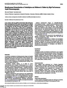
Our model consists of three variables: unemployment (u), GDP (y), and the budget balance (bb). Figure 1 describes the data.4 Traditional unit root tests suggest that u 5 The stationary vector of the variables and y are non-stationary hwhile bb is stationary. i 0 at hand is hence: ∆x = ∆u ∆y bb and the moving-average representation of the system is given by: ∆xt = µ + C(L)εt (1)
= µ + C0 εt + C1 εt−1 + C2 εt−2 + ... h
i
where µ = ∆x is a 3×1 vector of constants, L is a lag operator, and ε0t = εLM εPt εBC t t is a vector of (by assumption) orthogonal, unobserved structural shocks. The system is thus driven by three shocks. For many European countries (including Sweden), we believe that the following identification scheme (including the necessary three assumptions) is a fair description of reality: ): Owing to factors like changes in social security systems, 1. Labor Market Shock (εLM t the structure of the economies, demography, and hysteresis, we believe that the vertical long-run Phillips curve (and thereby the long-run aggregate supply curve) 4
The official unemployment rate is used. Hence, unemployed people participating in labor-market programs are not included. The series is taken from publications by Statistics Sweden. The GDP series is taken from the NIER. The budget balance, which concerns the consolidated government sector, is the measure to which the Stability and Growth Pact applies. This series is taken from the Statistical Yearbook (various issues) and the NIER. 5
The ADF statistics for unemployment and GDP are −3.2 and −3.1, respectively. Since the critical value when including a linear trend is −3.5, we could not reject the null of non-stationarity for these two series. (We also estimated the unemployment series without a trend but could not reject the null of non-stationarity: test value −2.6, critical value −2.9). The ADF statistic for the budget balance is −3.8; we could therefore reject the null of non-stationarity as the critical value when including a constant is −2.9. The most parsimoneous model with no autocorrelation (using Lagrange multiplier tests) is applied.
3
has shifted in many European countries since the 1950s. This shock corresponds to such shifts and, as the level of GDP is closely related to the labor market, we impose no restrictions on this shock. It is thus allowed to affect both unemployment and GDP in the long run.6 2. Productivity Shock (εPt ): This shock concerns shifts in the aggregate supply curve due to productivity shocks. While allowing such shocks to have long-run effects on GDP, we assume that there are no long-run effects on unemployment (1st assumption). Hence, our model suggests that, over the long run, the level of unemployment is determined only by the structure of the labor market, not by the development of productivity. 3. Business-cycle Shock (εBC t ): This shock is a traditional business-cycle shock (or, equally, a ’demand shock’), and we assume that it has no long-run effects on neither unemployment nor GDP (2nd and 3rd assumptions). As the structural shocks are not observed, an unrestricted VAR (UVAR) model must be estimated in order to recover the reduced-form shocks. The associated moving average representation equals: ∆xt = µ + R(L)υ t (2)
= µ + υ t + R1 υ t−1 + R2 υ t−2 + ...
where υ t is a 3 × 1 vector of reduced-form shocks. Equations (1) and (2) imply a linear relationship between the structural and reduced-form residuals: εt = C(L)−1 R(L)υ t .
(3)
By imposing the three mentioned long run restrictions above, we have the following long run representation of equation (1):
∆ut ∆yt = µ + C(1)εt bbt
P
∞ µu 0 0 εLM k=0 c11 (k) t P∞ P∞ P = µy + k=0 c21 (k) 0 εt , k=0 c22 (k) P∞ P∞ P∞ µbb εBC t k=0 c31 (k) k=0 c32 (k) k=0 c33 (k)
(4)
P
LM where C(1) is the long-run impact matrix and ∞ k=0 c11 (k)εt−k is the long-run effects of 7 labor-market shocks on ∆ut etc. Hence, the business cycle shock (εBC t ) is restricted by 6
As the budget balance is stationary, there are, by definition, no long run effects on this variable for any of the shocks. 7
As R(0) = I in (2), we note that C(0)εt = R(0) and R(j)C(0) = C(j). Our aim is to find C(0) so that C(L), and thereby the structural shocks, can be recovered through equation (3) in the main text.
4
having no long-run effects on unemployment and GDP, and the productivity shock (εPt ) is restricted by having no long-run effects on unemployment. It is well known that these three restrictions/assumptions cannot be tested statistically. We can, however, examine how the variables respond to the shocks. If they respond as we would expect from the labelling of the shocks, support (but no proof) is provided for the identification (and interpretation) of the system. As can be seen in Figure 2, u responds positively, while y and bb respond negatively, to an adverse labor-market shock; u responds negatively, while y and bb respond positively, to a favorable productivity shock; u responds negatively, while y and bb respond positively, to a favorable business-cycle shock. Hence, all responses are consistent on the identification (and thereby interpretation) of the model. Based on the identification described above, we obtain our three unobservable variables by calculating the historical decomposition in the following way: • NAIRU : what would the unemployment series look like in absence of productivity and business-cycle shocks? • Potential GDP ( y ∗ ): what would the GDP series look like in absence ³ of business ´ cycle shocks? The output gap is then calculated using the formula: yy∗ − 1 ∗ 100.
• Structural budget balance ( sbb): what would the budget balance series look like in absence of business-cycle shocks? The structural budget balance shown in the figures is calculated as a percentage of potential GDP. We can also note that: R(1)C(0) = C(1),
(5)
where C(1) = C0 + C1 + C2 + ... (same analogy for R(1)) represents the long-run effects from the shocks on the variables in the model. Estimation of the UVAR model generates Σ = υ t υ0t . Assuming that the structural shocks are orthogonal and normalizing their variance to one, we find that their variancecovariance matrix is equal to the identity matrix (ε0 ε = I). Using this fact and that υ t = C0 εt , we have: (6) C0 C00 = Σ. If we combine (5) and (6) we obtain: C(1)C(1)0 = R(1)ΣR(1)0 .
(7)
Letting H be the lower triangular Choleski decomposition of the right hand side of (7), we can recover C(0) through: C(0) = R(1)−1 H. The implication of C(1) = H is shown in equation (4) in the main text.
5
3
Swedish Evidence
Yearly data for the period 1950-2004 are available if the forecasts of the NIER are included.8 It is clear that the unemployment series contain a number of extreme data points for the years 1993-99 when unemployment is above 5% (see Figure 1). We believe it is unlikely that the data-generating process for this period is the same as for the rest of the sample. Probably no available model, including the present one, can fully account for this period in a satisfactory manner. Two models are therefore specified and estimated: one including a dummy that (to at least some extent) accounts for the ’extreme’ changes in unemployment during the 1990s, and another not including this dummy.9 Results obtained from both models will be presented below. While it is largely a matter of judgment which model is best, we believe that the model including the dummy presents the most realistic overall picture.10
3.1
Results
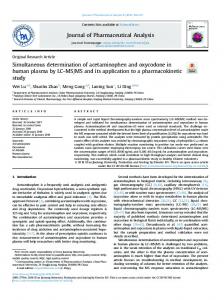
The results are displayed in Figure 3 and Table 1. In the right column of Figure 3, the two specifications (with and without the dummy) are compared for the period 1980-2004. Although the general picture is the same, there are some important differences. The average NAIRU estimate is about 4.8% for the period 1993-1997 in the model including the dummy and 6.3% in the model without the dummy. Hence, the dummy captures about 1.5 percentage points of the unemployment rate for this period. The differences between the models decrease considerably after this extreme period; the estimates imply a NAIRU of 3.7% and 4.3%, respectively, for the period 2002-2004 (see Table 1). The output gap was naturally greater during the crises in the 1990s, according to the model including the dummy, as NAIRU is lower in this model. At the end of the period 8
We use four lags which implies that the null of no (multivariate) autocorrelation and (multivariate) normality, respectively, could not be rejected using standard significance levels (see Lütkepohl, 1993, for details concerning these tests). DeSerres and Guay (1995) show that when some shocks only have temporary effects on one of the variables (as is true in our application), the VAR representation will in general contain an MA term. They also show that by implication the number of lags required to generate a fair decomposition of the structural shocks and the dynamics increases. 9
The unemployment variable is in first differences, and the size of the following dummy is determined by the size of the change in the variable in the respective years: D = 1 in 1993 when unemployment rose by 3 percentage points to 8.2%; D = −0.5 in 1998 when unemployment fell by 1.5 percentage points to 6.5%; D = −0.25 in 1999 when unemployment fell back by 0.9 percentage points to 5.6% - i.e. approximately the level before the big hump. As the dummies sum to 0.25 (1 − 0.5 − 0.25), the model allows for a level shift overall, which appears to be consistent with the data. As all three variables in the system are endogenous, the dummy will affect the other two variables as well. This is not a drawback as the dummy influence the NAIRU, which in turn is a central ingredient when calculating potential GDP and the structural budget balance. 10
The dummy is significant at the 1% and 10% levels, respectively, in the ∆u and ∆y equations (tvalues: 4.0 and −1.8, respectively) but insignificant in the bb equation (t-value: −1.4).
6
in the sample, the estimates are generally rather similar; thus, the average output gap is estimated at −0.7% and −0.5%, respectively, for the period 2002-2004. The estimates of the structural budget balance are rather similar in the two models. The greatest differences occur during 1998-2001, when the model including the dummy predicts a lower structural balance (0.8% on average compared to 1.8%). For the period 2002-2004, the average estimates are the same; see Table 1.
3.2
Interpretation
As mentioned above, the historical decomposition used to calculate the three variables above depends on the structural shocks. One benefit of using a SVAR approach is that one can analyze these time series of structural shocks (i.e., labor-market, productivity, and business-cycle shocks) and get information about their timing and relative magnitude. For example, by analyzing the shocks in the beginning of the 1990s we get some information of the causes of the deep recession during this period. It is important to remember, however, that the relationship between the variables and the shocks are not that straightforward because some shocks are allowed to have an long run impact on some of the variables. For example, all labor-market shocks except those after year t (see Figure 411 ), influence the NAIRU in year t. Their relative importance are determined by (a) the magnitude of the relevant impulse-response function (see Figure 2) and (b) the size of the shock (see Figure 4). In the calculation of the NAIRU, the labor-market shocks are the only ones having an effect, as neither productivity nor business-cycle shocks are assumed to have any impact on unemployment in the long run. Acknowledging that positive shocks correspond to unfavorable changes in behavior on the labor market, we see in Figure 4 that the periods 1990-1992 and 1995-96 were characterized by relatively large unfavorable labor-market shocks. We can also note the series of favorable (i.e. negative) labor-market shocks during the end of the sample period; these partly explain the rather low NAIRU estimates for the period 2002-2004. Productivity shocks are allowed to have long-run effects on GDP. It is interesting to note that productivity shocks do not appear to have played a significant role in the crises in the early 1990s. It is noteworthy, on the other hand, that several negative productivity shocks occurred in the mid-1970s, a fact consistent with common belief concerning a productivity slowdown during that period. Most importantly, however, several favorable productivity shocks occurred in the end of the sample. This is promising for the future as the effects of these shocks (most notably, the increase of potential GDP) will carry on for several years after 2004. One has to remember, however, that for the period 2002-2004, the estimated shocks as well as the three estimated unobservable variables rely on NIER’s 11
These shocks are taken from the model including the dummy. The shocks from the alternative model show a similar pattern.
7
forecasts of unemployment, GDP, and budget balance. Finally, the business-cycle shocks are relatively large and negative in the beginning of the 1990s. By comparing the business-cycle shocks for the 1960s and 1990s, one can easily understand the different macroeconomic outcomes. In the 1960s, the vast majority of the business-cycle shocks were favorable, whereas the opposite was true in the 1990s. One could also note that the upturn at the end of the 1990s cannot be explained by positive business cycle shocks at that time (as they are mainly negative) but rather by the favorable labor-market and productivity shocks discussed above.
4
Comparison with the OECD, the NIER, and the HP Filter
In this section we compare the results of our preferred model (i.e., including the dummy) with those of the OECD and the NIER.12 As the Hodrick-Prescott (HP) filter is commonly used to calculate output gaps, we will also include the HP gap in the comparison with SVAR. Unlike the present study, the OECD and the NIER estimate the variables in different models. In short, the approaches are the following: • NAIRU : The OECD uses a Kalman-filter approach on reduced-form Phillips curve equations (see Richardson et al, 2000). The NIER publishes a somewhat related measure, the so-called ’labor-market gap’ based on a production function approach in which only labor-market variables (unemployment, average working hours, and labor supply) are allowed to deviate from long run values (see Börjesson et al, 1999). • Output gap: The OECD and the NIER use a (Cobb-Douglas) production function approach where the actual capital stock, HP-filtered total factor productivity, and potential employment (including NAIRU, or NAWRU, estimates) are included in order to calculate the output gap (see Giorno et al, 1995, for the OECD measure, and Börjesson et al (1999) for the NIER measure). The HP filter (see Hodrick and Prescott, 1997) is basically a smoothing procedure and is obtained by minimizing the gap between output and potential output and the rate of change in potential output. • Structural budget balance: Here the OECD makes use of the estimated output gap referred to above and, together with estimated tax and spending elasticities, calculates the structural budget balance (see Giorno et al, 1995, and van den Noord, 2000). 12
The NIER does not publish any measure of NAIRU or structural budget balance. It does, however, publish a ’labor market gap’ based on a production-function approach which will be compared with our ’labor market gap’: u∗ − u.
8
4.1
Output gap
Beginning with the output-gap estimates, we have four measures: SVAR, NIER, OECD, and HP. Broadly, the four output gaps move together over the sample, but there are some important differences. As it can be difficult to trace the four output-gap measures in the same graph, we compare the SVAR estimates with the three others in separate graphs, see the right column in Figure 5. In the upper-right and mid-right graphs in Figure 5, SVAR is compared with NIER and OECD13 , respectively. The SVAR gap is less positive during the 1980s while the three gaps are rather similar from 1992 and onwards. One may note that the NIER gap is slightly more positive around the year 2000. The HP gap is different at the end of the sample period as it predicts a positive gap from 1999 and onwards. Hence, the interpretation of the present situation of the economy would be rather different if based on the HP filter. The average gap for the period 2002-2004 is −0.7, −0.6, −0.4, and 0.2 percent for the SVAR, OECD, NIER, and HP gaps, respectively.
4.2
NAIRU
For the OECD, we only have NAIRU estimates up to 1999; see the upper-left graph in Figure 5. For the whole period (1980-1999), the OECD estimates are one to two percentage points higher. If the dummy in the SVAR model is excluded, we find approximately the same pattern as with the OECD during the 1990s; see the upper-right graph of Figure 3. As mentioned, the ’labor-market gap’ published by the NIER does not imply an estimate of NAIRU but rather an output gap when just labor-market variables are allowed to differ from their potential level; see Börjesson et al (1999). We believe, however, that it is of some interest to compare this gap to the labor-market gap generated from the SVAR model (i.e., u∗ − u). As can be seen in the mid-left graph in Figure 5, the two labor-market gaps follow each other closely. The only exception is some larger differences at the end of the 1980s. The labor-market gap is on average −0.5% in the SVAR model and −0.4% in the NIER approach for the period 2002-2004.
4.3
Structural Budget Balance
For the estimates of structural budget balances, the important differences between SVAR and OECD begin in the period 1993-1995 when the structural deficit was −4.4, −3.7, and −2.0, respectively, according to the SVAR model whereas the counterparts for the OECD were −7.1, −7.9, and −6.0. Hence, a larger share of the total deficit is explained by the business cycle in the SVAR model. One important reason for this result is that the SVAR model, by comparison to the OECD, implied a smaller increase in the NAIRU. This in 13
Note that the OECD gap ends in 2003.
9
turn implies a more limited impact on the budget balance from the NAIRU, a structural factor that partly determines the structural deficit. A general result is that the structural budget balance of the OECD follows the actual budget balance much more closely than the SVAR model. This implies that cyclical factors explain more of the variation in the budget balance in the SVAR model than in the OECD approach.
4.4
The Sensitivity of Inflation to Output Gaps
One important reason for estimating output gaps is their assumed relationship to inflation. More specifically, it is often believed that, for yearly data, a positive gap in t implies higher level of inflation in t + 1. A simple Phillips curve, augmented for expected inflation, could be expressed as (see Coe and McDermott, 1997): π t = α0 + π et +
k X
β i gapt−i + εt ,
i=0
where π, π e , and gap is inflation, inflation expectations in t, and output gap, respectively. We allow for a flexible degree of adaptive expectations (πe = α1 π t−1 ) and, based on pretesting of lag length, the gap is measured in t − 1. Finally, we present results both excluding and including a dummy (D) that equals one from 1992 and onwards. The reason for this dummy (which always is significant in the regressions; see Table 2) is the sharp and persistent level shift of the inflation rate in 1992. Hence, the following equation is estimated for the four output gaps: π t = α0 + α1 π t−1 + α2 gapt−1 + α3 Dt + εt . The sensitivity of inflation to the four different output gaps is very similar; see Table 2. When the dummy is excluded, α2 lies between 0.30 (HP) and 0.39 (SVAR). Hence, an output gap of 1% in year t implies an increase in the inflation rate by 0.30 − 0.39 percentage points in t + 1, according to the four models. When we include the dummy, which is always significant and raises R2 considerably, α2 then lies between 0.09 (SVAR and NIER) and 0.11 (OECD), and the significance disappears. It is not strange that the dummy plays an important role in view of the persistent decline in the inflation rate in the early 1990s. Finally, we may note that the NIER estimates imply a higher R2 compared to the other models.
5
Conclusions
In this paper we suggest a new method that estimates NAIRU, output gaps, and structural budget balances in the same model using a structural VAR (SVAR) approach. We consider this feature important as it is principally the effects of the same business cycle that are to be removed from the three series. The method is designed to take the non-stationarity of 10
(primarily) European unemployment into account by allowing for labor market shocks to have long run effects on the unemployment rate and hence the NAIRU. Another strength of the suggested SVAR approach is that it makes it possible to evaluate the estimates based on the time series of structural shocks. For example, our application shows that the sharp downturn in Sweden in the beginning of the 1990s was primarily due to adverse labor market and business cycle shocks rather than adverse productivity shocks. In conclusion, two SVAR models are estimated and the results concerning NAIRU, potential growth, output gap, and structural budget balance are summarized in Table 1. We can note that for the projection period 2002-2004, the average NAIRU, potential growth rate, output gap, and structural budget balance for the preferred model are estimated at 3.7%, 2.1%, −0.7%, and 1.7%, respectively. There are also a number of weaknesses to the present SVAR approach. First, owing to the lag structure, this approach is rather data-intensive and requires long data series. As quarterly data on the consolidated budget balance (i.e. the variable concerned by the Stability and Growth Pact) for reasonably long periods is not available in most countries, one has to rely on yearly data. As a result, the series must start around the 1950s. Since the budget balance of the consolidated government sector is not published in any official source for such a long period, one has to search for series in printed material and combine different sources at national statistical offices, a cumbersome procedure if the study is to cover many countries. By comparison, the OECD approach to calculate the structural budget balance in recent years calls only for data on the budget balance for the years in question, whereas data for GDP are required (and are available) for a longer period in order to calculate potential GDP. A second problem with the SVAR approach is that there are more ’humps’ to pass in order to carry out the analysis than is the case, for example, in calculating an output gap with a production function approach. The series must also meet the integration tests if the shocks and the model are to be given the same interpretation as we use in this paper. Moreover, applying the present interpretation of the model requires that the signs of the impulse-response functions be the same as the ones presented in this paper. Despite these weaknesses, the suggested unifying method could be useful as a complement to the existing methods applied by the OECD and other research institutes. As the three series are unobservable, their believed sizes are to an important extent a matter of judgement. In this process of judgement, we believe it would be wise to use and weigh information arising from several models.
11
References Apel, M., Jansson, P., 1999a. System Estimates of Potential Output and the NAIRU. Empirical Economics 24:373-388. Apel, M., Jansson, P., 1999b. A Theory Consistent Approach for Estimating Potential Output and the NAIRU. Economics Letters 64:271-275. Blanchard, O.J., Quah, D., 1989. The Dynamic Effects of Aggregate Demand and Supply Disturbances. American Economic Review 79:655-73. Boone, L., 2000. Comparing Semi Structural Methods to Estimate Unobserved Variables: the HPMV and Kalman Filters Approaches. OECD ECO/WKP 13. Börjesson, P-L., Hofvander, N., Lindén, J., 1999. Potentiell produktion och produktionsgap (in Swedish). Konjunkturläget, November 1999. (In Swedish). Cerra, V., Saxena, S.C., 2000. Alternative Methods of Estimating Potential Output and the Output Gap: an Application to Sweden. IMF Working Paper 59. Coe, D.T., McDermott, C.J., 1997. Does the Gap Model Work in Asia? IMF Staff Papers, vol.44, no. 1 (March). DeSerres, A., Guay, A., 1995. Selection of the Truncation Lag in Structural VARs (or VECMs) with Long Run Restrictions. Bank of Canada Working Paper 95-9. European commission, 1995. Technical Note: the Commissions Services’ Method for the Cyclical Adjustment of Government Budget Balances. European Economy. No 60. Giorno, C., Richardson, P., Roseveare, D., van den Noord, P., 1995. Estimating Potential Output, Output Gaps and Structural Budget Balances. OECD ECO/WKP 152. Hodrick, R., Prescott, E.C., 1997. Post War U.S. Business Cycles: an Empirical Investigation. Journal of Money, Credit and Banking 29:1-16. Hokkanen, J., 1998. Estimating Structural Budget Balances with Unobservable Components. Chapter 4 in the PhD thesis: Interpreting Budget Deficits and Productivity Fluctuations. Economic Studies 42, Uppsala University. IMF, 1993. Structural Budget Indicators for the Major Industrial Countries. World Economic Outlook, October. Lütkepohl, H., 1993. emph{Introduction to Multiple Time Series Analysis. SpringerVerlag. Germany. 12
Mc Morrow, K., Roeger, W., 2000. Potential Output: Measurement Methods, ”New Economy” Influences and Scenarios for 2001-2010 - A Comparison of the EU15 and US. European Commission. Economic Papers No. 150. Mc Morrow, K., Roeger, W., 2000. Time Varying NAIRU/NAWRU Estimates for the EU’s Member States. European Commission. Economic Papers No. 145. Richardson, P., Boone, L., Giorno, C., Meacci, M., Rae, D., Turner, D., 2000. The Concept, Policy Use and Measurement of Structural Unemployment: Estimating a Time Varying NAIRU Across 21 OECD Countries. OECD ECO/WKP 23. Scott, A., 2000. Stylized Facts from Output Gap Measures. Reserve Bank of New Zealand. Discussion Paper Series No. 7. St-Amant, P., van Norden, S., 1997. Measurement of the Output Gap: A Discussion of Recent Research at the Bank of Canada. Working Paper No. 79, Bank of Canada. van den Noord, P., 2000. The Size and Role of Automatic Fiscal Stabilizers in the 1990s and Beyond. OECD ECO/WKP 3.
13
Table 1: Summary of Results Using the SVAR Model
1955-59 1960-64 1965-69 1970-74 1975-79 1980-84 1985-89 1990-94 1995-99 2000-04
NAIRU (D) (no D) 2.7 2.8 1.6 1,7 2.4 2.8 3.1 3.7 1.5 1.6 2.2 1.5 2.1 2.0 3.9 4.8 4.9 6.0 4.0 4.6
5-YEAR AVERAGE Pot.Growth Output gap (D) (no D) (D) (no D) 3.3 3,2 0.7 0,9 4.5 4,4 1.0 1,4 3.6 3.6 2.9 3.8 3.8 3.8 2.8 3.3 2.2 2.4 -0.6 -0.8 2.2 2.2 -1.9 -2.6 2.1 1.8 -0.2 0.1 1.5 1.3 -2.0 -1.2 2.0 2.5 -1.9 -1.4 2.4 2.3 -0.3 -0.1
Str.Balance (D) (no D) -0.6 -0,7 1.9 1,4 -1.3 -1.9 -0.4 -0.1 3.1 3.5 -1.4 -0.9 0.9 0.1 -2.3 -2.8 -0.1 -0.0 1.5 1.9
2002 2003 2004 2002-04
3.6 3.7 3.8 3.7
PREDICTION YEARS 2.3 2.2 -0.8 -0.4 2.0 2.2 -1.0 -0.9 2.0 2.0 -0.3 -0.2 2.1 2.1 -0.7 -0.5
1.8 2.0 1.4 1.7
Years
4.3 4.2 4.3 4.3
1.9 1.9 1.3 1.7
Note: ’(D)’: model including a dummy. ’(no D)’: model without a dummy. ’Pot.Growth’: potential growth. A positive output gap implies that current output is above potential output. ’Str.Balance’: structural budget balance as a percentage of potential GDP.
14
Table 2: Inflation and Output Gaps: SVAR, OECD, NIER, and HP Variables Constant
Coeff. α0
π t−1
α1
gapt−1
α2
D
α3
R2
SVAR 1.52* 5.01* (0.72) (1.13) 0.77* 0.42* (0.10) (0.13) 0.39* 0.09 (0.17) (0.17) -4.01* (1.11) 0.69
0.78
OECD 1.43** 4.87* (0.79) (1.29) 0.79* 0.43* (0.10) (0.14) 0.35* 0.11 (0.17) (0.16) -3.92* (1.25) 0.70
0.78
HP 1.23** 5.03* (0.72) (1.11) 0.78* 0.41* (0.10) (0.13) 0.30** 0.10 (0.18) (0.16) -4.14* (1.02) 0.67
0.79
NIER 1.34** 4.33* (0.71) (1.16) 0.68* 0.41* (0.11) (0.13) 0.37** 0.09 (0.21) (0.20) -3.39* (1.13) 0.74
0.82
Note: Dependent variable: inflation (based on Consumer Price Index). Effective time period: 1971-2004 (1971-2003 is used for the OECD and 1980-2004 for the NIER because of data availability). ’HP’ use the output gap based on the HP filter, lambda=100. ’D’ is a dummy that equals one for the period 1992-2004, zero otherwise. Standard errors in parentheses. ’*’, ’**’ denote significance at the 5- and 10-percent level, respectively.
15
Figure 1: The Data: Official Unemployment Rate, GDP and Consolidated Budget Balance (base year: 2001). Period 1950-2004. Official Unemployment Rate 9 8 7
Percent
6 5 4 3 2 1 1950 1954 1958 1962 1966 1970 1974 1978 1982 1986 1990 1994 1998 2002
GDP 2500000 2250000 2000000
Millions SEK
1750000 1500000 1250000 1000000 750000 500000 1950 1954 1958 1962 1966 1970 1974 1978 1982 1986 1990 1994 1998 2002
Budget Balance 100000 50000
Millions SEK
0 -50000 -100000 -150000 -200000 -250000 1950 1954 1958 1962 1966 1970 1974 1978 1982 1986 1990 1994 1998 2002
16
Figure 2: Impulse Responses of Unemployment (u), GDP and the Budget Balance (bb) to Three Structural Shocks. (years after the shock on the horizontal axis). u Response to a Labor Market Shock
u Response to a Productivity Shock
0.575
u Response to a Business Cycle Shock
0.025
0.10
0.05
-0.000
0.550
-0.00 -0.025 0.525 -0.05 -0.050 0.500
-0.10 -0.075 -0.15
0.475 -0.100 -0.20 0.450
-0.125
0.425
-0.25
-0.150 0
3
6
9
12
15
18
21
24
-0.30 0
GDP Response to a Labor Market Shock
3
6
9
12
15
18
21
24
GDP Response to a Productivity Shock
-3200
6
9
12
15
18
21
24
15000
23000
12500
22000
-6400
3
GDP Response to a Business Cycle Shock
24000
-4800
0
10000
21000 -8000
7500 20000
-9600
5000 19000
-11200
2500 18000
-12800
0
17000
-14400
16000 0
3
6
9
12
15
18
21
24
-2500 0
bb Response to a Labor Market Shock
3
6
9
12
15
18
21
24
bb Response to a Productivity Shock
0
2700
30000
2500
1800
25000
900
20000
-2500
0
15000
-5000
-900
10000
5000
-7500
-1800
-10000
-2700
-12500
-3600
-5000
-15000
-4500
-10000
0
3
6
9
12
15
18
21
24
6
9
12
15
18
21
24
21
24
bb Response to a Business Cycle Shock
5000
0
3
0
0
3
6
9
12
17
15
18
21
24
0
3
6
9
12
15
18
Figure 3: Left column: Results from the Model Including the Dummy Variable (’_D_’). Right column: Comparison with Results Without the Dummy. Unemployment and NAIRU
NAIRU: With and Without Dummy (D)
9
8.4
U
U
SVAR_D_NAIRU
SVAR_D_NAIRU
8
SVAR_NAIRU
7.2
7
6.0
6
Percent
Percent
4.8 5 4
3.6
2.4
3
1.2
2 1
0.0 1955
1960
1965
1970
1975
1980
1985
1990
1995
2000
1980
Output Gap
1983
1986
1989
1992
1995
1998
2001
2004
Output Gap: With and Without Dummy (D)
3.6
2.7
2.4
1.8
SVAR_D_GAP SVAR_GAP
0.9
1.2
-0.0
0.0
Percent
Percent
-0.9 -1.2 -2.4 -3.6
-1.8 -2.7 -3.6
-4.8
-4.5
-6.0
-5.4 1955
1960
1965
1970
1975
1980
1985
1990
1995
2000
1980
Structural (SBB) and Actual (BB) Budget Balance
1983
1986
1989
1992
1995
1998
2001
2004
Structural Budget Balance: With and Without Dummy (D)
6
5.0
4
2.5
2
Percentage of (for SBB potential) GDP
Percentage of (for SBB, potential) GDP
0.0 0 -2 -4 -6 -8 -10
BB SVAR_D_SBB
-12 1955
1960
1965
1970
1975
1980
1985
1990
1995
2000
18
-2.5
-5.0
-7.5
-10.0
BB SVAR_D_SBB SVAR_SBB
-12.5 1980
1983
1986
1989
1992
1995
1998
2001
2004
Figure 4: The Time Series of Structural Shocks in the Model Including the Dummy. Labor Market Shocks (+ for unfavorable shock) 3 2 1 0 -1 -2 1955
1959
1963
1967
1971
1975
1979
1983
1987
1991
1995
1999
2003
1995
1999
2003
1995
1999
2003
Productivity Shocks (+ for favorable shock) 2.4 1.6 0.8 -0.0 -0.8 -1.6 -2.4 1955
1959
1963
1967
1971
1975
1979
1983
1987
1991
Business Cycle Shocks (+ for favorable shock) 2.4 1.6 0.8 -0.0 -0.8 -1.6 -2.4 1955
1959
1963
1967
1971
1975
1979
19
1983
1987
1991
Figure 5: Comparison of Results: SVAR, OECD, NIER, and HP. NAIRU: SVAR and OECD
Output Gap: SVAR and NIER
9
2.7 U SVAR_D_NAIRU
8
1.8
OECD_NAIRU
0.9
7
-0.0
6
Percent
Percent
-0.9 5 4 3
-1.8 -2.7 -3.6
2
-4.5
NIER_GAP SVAR_D_GAP
1
-5.4 1980
1983
1986
1989
1992
1995
1998
2001
2004
1980
Labor Market Gap: SVAR and NIER
1983
1986
1989
1992
1995
1998
2001
2004
Output Gap: SVAR and OECD
3
4 NIER_U_GAP SVAR_U_GAP
2 2 1 0
Percent
Percent
0
-1
-2
-2 -4 -3 OECD_GAP
-4
SVAR_D_GAP
-6 1980
1983
1986
1989
1992
1995
1998
2001
2004
1980
Structural Budget Balance: SVAR and OECD
1983
1986
1989
1992
1995
1998
2001
2004
Output Gap: SVAR and HP
6
4.2
4
2.8
2
0.0
-2
Percent
Percentage of (for SBB potential) GDP
1.4 0
-4 -6
-1.4
-2.8 -8 -4.2
BB
-10
SVAR_D_SBB
HP_GAP
OECD_SBB
-12 1980
1983
1986
1989
1992
1995
1998
2001
SVAR_D_GAP
-5.6 2004
1980
20
1983
1986
1989
1992
1995
1998
2001
2004
Titles in the Working Paper Series No
Author
Title
Year
1
Warne, Anders and Anders Vredin
Current Account and Business Cycles: Stylized Facts for Sweden
1989
2
Östblom, Göran
Change in Technical Structure of the Swedish Economy
1989
3
Söderling, Paul
Mamtax. A Dynamic CGE Model for Tax Reform Simulations
1989
4
Kanis, Alfred and Aleksander Markowski
The Supply Side of the Econometric Model of the NIER
1990
5
Berg, Lennart
The Financial Sector in the SNEPQ Model
1991
6
Ågren, Anders and Bo Jonsson
Consumer Attitudes, Buying Intentions and Consumption Expenditures. An Analysis of the Swedish Household Survey Data
1991
7
Berg, Lennart and Reinhold Bergström
A Quarterly Consumption Function for Sweden 1979- 1991 1989
8
Öller, Lars-Erik
Good Business Cycle Forecasts- A Must for Stabilization Policies
1992
9
Jonsson, Bo and Anders Ågren
Forecasting Car Expenditures Using Household Survey Data
1992
10
Löfgren, Karl -Gustaf, Bo Ranneby and Sara Sjöstedt
Forecasting the Business Cycle Not Using Minimum Autocorrelation Factors
1992
11
Gerlach, Stefan
Current Quarter Forecasts of Swedish GNP Using Monthly Variables
1992
12
Bergström, Reinhold
The Relationship Between Manufacturing Production and Different Business Survey Series in Sweden
1992
13
Edlund, Per-Olov and Sune Karlsson
Forecasting the Swedish Unemployment Rate: VAR vs. Transfer Function Modelling
1992
14
Rahiala, Markku and Timo Teräsvirta
Business Survey Data in Forecasting the Output of Swedish and Finnish Metal and Engineering Industries: A Kalman Filter Approach
1992
15
Christofferson, Anders, Roland Roberts and Ulla Eriksson
The Relationship Between Manufacturing and Various BTS Series in Sweden Illuminated by Frequency and Complex Demodulate Methods
1992
16
Jonsson, Bo
Sample Based Proportio ns as Values on an Independent Variable in a Regression Model
1992
17
Öller, Lars-Erik
Eliciting Turning Point Warnings from Business Surveys
1992
18
Forster, Margaret M
Volatility, Trading Mechanisms and International Cross-Listing
1992
19
Jonsson, Bo
Prediction with a Linear Regression Model and Errors in a Regressor
1992
20
Gorton, Gary and Richard Rosen
Corporate Control, Portfolio Choice, and the Decline of Banking
1993
21
Gustafsson, ClaesHåkan and Åke Holmén
The Index of Industrial Production – A Formal Description of the Process Behind it
1993
22
Karlsson, Tohmas
A General Equilibrium Analysis of the Swedish Tax Reforms 1989-1991
1993
23
Jonsson, Bo
Forecasting Car Expenditures Using Household Survey Data- A Comparison of Different Predictors
1993
21
24
Gennotte, Gerard and Hayne Leland
Low Margins, Derivative Securitites and Volatility
1993
25
Boot, Arnoud W.A. and Stuart I. Greenbaum
Discretion in the Regulation of U.S. Banking
1993
26
Spiegel, Matthew and Deane J. Seppi
Does Round-the-Clock Trading Result in Pareto Improvements?
1993
27
Seppi, Deane J.
How Important are Block Trades in the Price Discovery Process?
1993
28
Glosten, Lawrence R.
Equilibrium in an Electronic Open Limit Order Book
1993
29
Boot, Arnoud W.A., Stuart I Greenbaum and Anjan V. Thakor
Reputation and Discretion in Financial Contracting
1993
30a
Bergström, Reinhold
The Full Tricotomous Scale Compared with Net Balances in Qualitative Business Survey Data – Experiences from the Swedish Business Tendency Surveys
1993
30b
Bergström, Reinhold
Quantitative Production Series Compared with Qualiative Business Survey Series for Five Sectors of the Swedish Manufacturing Industry
1993
31
Lin, Chien-Fu Jeff and Timo Teräsvirta
Testing the Constancy of Regression Parameters Against Continous Change
1993
32
Markowski, Aleksander and Parameswar Nandakumar
A Long-Run Equilibrium Model for Sweden. The Theory Behind the Long-Run Solution to the Econometric Model KOSMOS
1993
33
Markowski, Aleksander and Tony Persson
Capital Rental Co st and the Adjustment for the Effects of the Investment Fund System in the Econometric Model Kosmos
1993
34
Kanis, Alfred and Bharat Barot
On Determinants of Private Consumption in Sweden
1993
35
Kääntä, Pekka and Christer Tallbom
Using Business Survey Data for Forecasting Swedish Quantitative Business Cycle Varable. A Kalman Filter Approach
1993
36
Ohlsson, Henry and Anders Vredin
Political Cycles and Cyclical Policies. A New Test Approach Using Fiscal Forecasts
1993
37
Markowski, Aleksander and Lars Ernsäter
The Supply Side in the Econometric Model KOSMOS 1994
38
Gustafsson, ClaesHåkan
On the Consistency of Data on Production, Deliveries, and Inventories in the Swedish Manufacturing Industry
1994
39
Rahiala, Markku and Tapani Kovalainen
Modelling Wages Subject to Both Contracted Increments and Drift by Means of a SimultaneousEquations Model with Non-Standard Error Structure
1994
40
Öller, Lars-Erik and Christer Tallbom
Hybrid Indicators for the Swedish Economy Based on 1994 Noisy Statistical Data and the Business Tendency Survey
41
Östblom, Göran
A Converging Triangularization Algorithm and the Intertemporal Similarity of Production Structures
1994
42a
Markowski, Aleksander
Labour Supply, Hours Worked and Unemployment in the Econometric Model KOS MOS
1994
42b
Markowski, Aleksander
Wage Rate Determination in the Econometric Model KOSMOS
1994
43
Ahlroth, Sofia, Anders Björklund and Anders Forslund
The Output of the Swedish Education Sector
1994
44a
Markowski, Aleksander
Private Consumption Expendi ture in the Econometric Model KOSMOS
1994
22
44b
Markowski, Aleksander
The Input-Output Core: Determination of Inventory Investment and Other Business Output in the Econometric Model KOSMOS
1994
45
Bergström, Reinhold
The Accuracy of the Swedish National Budget Forecasts 1955-92
1995
46
Sjöö, Boo
Dynamic Adjustment and Long -Run Economic Stability
1995
47a
Markowski, Aleksander
Determination of the Effective Exchange Rate in the Econometric Model KOSMOS
1995
47b
Markowski, Aleksander
Interest Rate Determination in the Econometric Model KOSMOS
1995
48
Barot, Bharat
Estimating the Effects of Wealth, Interest Rates and Unemployment on Private Consumption in Sweden
1995
49
Lundvik, Petter
Generational Accounting in a Small Open Economy
1996
50
Eriksson, Kimmo, Johan Karlander and Lars-Erik Öller
Hierarchical Assignments: Stability and Fairness
1996
51
Url, Thomas
Internationalists, Regionalists, or Eurocentrists
1996
52
Ruist, Erik
Temporal Aggregation of an Econometric Equation
1996
53
Markowski, Aleksander
The Financial Block in the Econometric Model KOSMOS
1996
54
Östblom, Göran
Emissions to the Air and the Allocation of GDP: Medium Term Projections for Sweden. In Conflict with the Goals of SO2, SO 2 and NOX Emissions for Year 2000
1996
55
Koskinen, Lasse, Aleksander Markowski, Parameswar Nandakumar and LarsErik Öller
Three Seminar Papers on Output Gap
1997
56
Oke, Timothy and Lars-Erik Öller
Testing for Short Memory in a VARMA Process
1997
57
Johansson, Anders and Karl -Markus Modén
Investment Plan Revisions and Share Price Volatility
1997
58
Lyhagen, Johan
The Effect of Precautionary Saving on Consumption in Sweden
1998
59
Koskinen, Lasse and Lars-Erik Öller
A Hidden Markov Model as a Dynamic Bayesian Classifier, with an Application to Forecasting Business-Cycle Turning Points
1998
60
Kragh, Börje and Aleksander Markowski
Kofi – a Macromodel of the Swedish Financial Markets
1998
61
Gajda, Jan B. and Aleksander Markowski
Model Evaluation Using Stochastic Simulations: The Case of the Econometric Model KOSMOS
1998
62
Johansson, Kerstin
Exports in the Econometric Model KOSMOS
1998
63
Johansson, Kerstin
Permanent Shocks and Spillovers: A Sectoral Approach Using a Structural VAR
1998
64
Öller, Lars-Erik and Bharat Barot
Comparing the Accuracy of European GDP Forecasts
1999
65
Huhtala , Anni and Eva Samakovlis
Does International Harmonization of Environmental Policy Instruments Make Economic Sense? The Case of Paper Recycling in Europe
1999
66
Nilsson, Charlotte
A Unilateral Versus a Multilateral Carbon Dioxide Tax 1999 - A Numerical Analysis With The European Model GEM-E3
23
67
Braconier, Henrik and Steinar Holden
The Public Budget Balance – Fiscal Indicators and Cyclical Sensitivity in the Nordic Countries
1999
68
Nilsson, Kristian
Alternative Measures of the Swedish Real Exchange Rate
1999
69
Östblom, Göran
An Environmental Medium Term Economic Model – EMEC
1999
70
Johnsson, Helena and Peter Kaplan
An Econometric Study of Private Consumption Expenditure in Sweden
1999
71
Arai, Mahmood and Fredrik Heyman
Permanent and Temporary Labour: Job and Worker Flows in Sweden 1989-1998
2000
72
Öller, Lars-Erik and Bharat Barot
The Accuracy of European Growth and Inflation Forecasts
2000
73
Ahlroth, Sofia
Correcting Net Domestic Product for Sulphur Dioxi de and Nitrogen Oxide Emissions: Implementation of a Theoretical Model in Practice
2000
74
Andersson, Michael K. And Mikael P. Gredenhoff
Improving Fractional Integration Tests with Bootstrap Distribution
2000
75
Nilsson, Charlotte and Anni Huhtala
Is CO2 Trading Always Beneficial? A CGE-Model Analysis on Secondary Environmental Benefits
2000
76
Skånberg, Kristian
Constructing a Partially Environmentally Adjusted Net Domestic Product for Sweden 1993 and 1997
2001
77
Huhtala, Anni, Annie Toppinen and Mattias Boman,
An Environmental Accountant's Dilemma: Are Stumpage Prices Reliable Indicators of Resource Scarcity?
2001
78
Nilsson, Kristian
Do Fundamentals Explain the Behavior of the Real Effective Exchange Rate?
2002
79
Bharat, Barot
Growth and Business Cycles for the Swedish Economy
2002
80
Bharat, Barot
House Prices and Housing Investment in Sweden and the United Kingdom. Econometric Analysis for the Period 1970-1998
2002
81
Hjelm, Göran
Simultaneous Determination of NAIRU, Output Gaps and Structural Budget Balances: Swedish Evidence
2003
24