Networks for Target Monitoring. Ying Guo, Zhongwen Guo, Feng Hong, Lu Hong. Department of Computer Science and Engineering. Ocean University of China.
2009 Sixth IFIP International Conference on Network and Parallel Computing
Sleep Scheduling and Gradient Query in Sensor Networks for Target Monitoring Ying Guo, Zhongwen Guo, Feng Hong, Lu Hong Department of Computer Science and Engineering Ocean University of China QingDao, China Email: {guoying, guozhw, hongfeng, honglu}@ouc.edu.cn
new challenges to the design of duty cycling mechanisms to prolong the lifetime as far as possible, which include: • As the targets are moving in the deployment area, it should be carefully designed for the duty cycling algorithm to keep the targets being sensed while most of the nodes are in sleep. The key to this problem contains two questions, which can be divided as what kinds of sensor nodes can go to sleep and how long they can be in the sleep mode. • Another important operation is to answer the information of the targets in the sensor networks of target monitoring. So it is another nontrivial problem how to transfer the target information to answer user queries when most of nodes are sleeping. In this paper, we present the novel duty cycling design for the sensor networks of target monitoring. Our design includes two algorithms, which are Sleep Scheduling Algorithm (SSA) and Gradient Query Algorithm based on sleep period (GQA). SSA is exploited to find out the optimal sleep periods for every node to save energy and to ensure that the targets always be monitored when the target is moving, and most of the nodes are in sleep mode. GQA is to guarantee that all the nodes have to be waken up when the user queries are answered through the gradient query route. The gradient of GQA is based on the sleep periods of the sensor nodes, while the target information are always stored in the active nodes. Meanwhile, the route of GQA is the shortest path from the user to the information source through sleep periods decreased path. Major contributions of this paper can be summarized as follows: • We propose the novel duty cycle design for the sensor networks of target monitoring, which can prolong the lifetime of the network as far as possible, and can answer the target information queries through gradient query routing. • The performance of the proposed design has been evaluated through theoretical analysis and simulations, which prove the functionality of the proposed design on the reduction of energy consumption. The rest of this paper is organized as follows. Section II
Abstract—Duty cycling is an important method for energy constrained sensor networks to prolong its lifetime. Current researches on duty cycling are often based on such assumption that all the sensory coverage should be maintained while some nodes are sleeping. For the applications of target monitoring, however, it is not necessary anymore to keep the whole sensory coverage of the sensor networks. It only needs to make sure that such kinds of nodes are active which can perceive the activities of the monitored targets. This observation brings new challenges to the design of duty cycling for the sensor networks. This paper proposes the novel duty cycling design for the sensor networks of target monitoring, which includes two algorithms of the sleep scheduling algorithm and the gradient query algorithm based on sleep periods. Under the proposed design, most of the sensor nodes can be in sleep, while still keep the functions of target monitoring and target query in the sensor networks. The performance of our design has been evaluated through both theoretical analysis and simulations, which prove the functionality of the proposed design on the reduction of energy consumption. Index Terms—sleep scheduling; gradient query; target monitoring; energy saving; wireless sensor networks;
I. I NTRODUCTION Wireless sensor networks are deployed in the physical environments to monitor or detect targets, for which the constrained energy supply of the batteries of the sensor nodes is one fundamental bottleneck. Prolonging the lifetime of the sensor networks is a prime consideration in network design [1]. Current approaches of duty cycling allow some nodes to go to sleep without destroying sensory coverage. In order to satisfy the right degree of coverage, certain number of nodes must keep awake [2], [3], [4], [5]. Both random and synchronized sleep scheduling algorithms have been studied in depth [6], [7]. However, one important factor has been left out of consideration in the approaches mentioned above, that it does not always need to keep the sensory coverage for some certain kinds of applications. For example, the applications of target monitoring do not need all the deployment area be covered by the sensor nodes. It only needs to make sure that such kinds of nodes are active which can perceive the activities of the monitored targets, while a large number of the sensor nodes can go to sleep. This kind of sensor networks brings 978-0-7695-3837-2/09 $26.00 $25.00 © 2009 IEEE DOI 10.1109/NPC.2009.33
101
summarizes the related works on sleeping schedule and gradient query. Section III and IV present the design of SSA and GQA in details and analyze their performance theoretically. Section V discusses the case of multi-targets monitoring of the proposed design. Section VI presents the simulations and demonstrates the performance of SSA and GQA. Section VII concludes this paper.
to rendezvous with data in the network. Geographical hash tables (GHTs) [16] maps the target type to a geographical location by a content based hash function. However, the data retrieval scheme in [16] is not distance-sensitive. Improvement of the flat hashing by hierarchical hashing has been investigated with hash locations aware of data correlation in [17], [18], [19]. Similar data is stored closely, then nearby users can discover souse nodes more quickly. Double rulings [20] proposed a new scheme, which stores data replica at a curve instead of one or multiple isolated sensors and the user travels along another curve which guarantees to intersect with the source curve. Most gradient based routing [21], [22] use the natural gradients of physical phenomena, which are based on the spatial distribution of many physical quantities, such as temperature, illumination and so on. Gradients imposed by natural laws [23], [24], [25] can be far from perfect guides, as witnessed by the existence of local extreme or large plateau regions. Because forcing information-guided routing to deteriorate to a random walk [26]. Information gradients in [26], diffuse information away from source nodes holding desired data to establish information potentials. Network queries can navigate along these information potentials and reach the sources. [27] developed a gradient based routing scheme such that from any query node, the query message follows the signal field gradient or derived quantities and successfully discovers all iso-contours of interest. The novelty of GQA is that it dose not use natural gradient or processed information gradient, but makes use of sleep scheduling. GQA uses different sleep periods of nodes to make up sleep periods decrease gradient routes. Queries from users walk along these routes to get the data they interested. No redundancy transmission in the query process, because the route is the shortest path from the user to the source node.
II. R ELATED W ORK Lots of methods about sleeping schedule and gradient query have been proposed in wireless sensor networks. A. Sleeping Schedule As we know the energy consumption in sleep state is much smaller than in active and listen state, so taking nodes to sleep is an efficient method to save energy. Most of researches focus on taking nodes to sleep while maintaining full coverage, such as [2], [3], [4], [5]. Some of them focus on solving the problem of set k-coverage [8], [9], [10], which divide the network area into several subsets, each of the subsets can cover the whole monitoring area. So these approaches only keep one of the subsets in active state to satisfy full coverage. [11], [12] make use of the positional relationship of neighbor nodes and let redundant nodes to sleep. These methods need more than enough nodes to be deployed to guarantee sensing coverage, they are based on a specified degree of redundancy. Some researches focus on partial coverage based protocols [6], [7], [1]. These schemes are investigated to improve energy-efficiency. In [6] each node independently chooses random sleep and wake up times. In [7] all nodes go to sleep and wake up in a synchronized fashion. Both of them force on the problem of tracking moving targets, while [1] focus on stationary target detection and find a localized algorithm that approaches the minimum average delay bound. SSA is different from previous works, which makes use of the characteristic of target monitoring. All of the approaches mentioned above ignore the actual situation of target monitoring. They all focus on the coverage of the deployment area when some nodes are asleep. But in applications of target monitoring, it dose not need all the deployment area to be monitored, only the nodes which perceiving the target keep alive and others can go to sleep. As most of the nodes are in sleep state and no redundancy nodes to be deployed, SSA will save a lot of energy.
III. D ESIGN OF SSA We present the design of SSA in detail in this section. SSA is designed for sensor networks of target monitoring, and all the sensor nodes do not need to know their positions. There are two steps to implement SSA, one is initialization phase and another is state transformation phase. We will introduce these two steps in the following subsections separately. A. Initialization When nodes are deployed in the monitoring area, initialize time Ti and time slot Tu should be determined in advance. There are three states for nodes: active state, listen state and sleep state. Every node should decide its state inside Ti . If it will turn to sleep state, it also has to compute out the length of sleep period. Nodes decide their states and sleep periods as follows. After deployment, all the nodes begin to detect the target. If one node finds the target, it turns into active state and broadcasts the target (T) to others. The node which received (T) and doesn’t detect the target, turns to listen state and broadcasts the target and the number of hops from it to the target (T,n) to others, where n=0 for listen state node.
B. Gradient Query Many approaches about information storage and query have been proposed in sensor networks [13]. In directed diffusion [14] information discovery through a reactive approach, which allows the query node to flood its interests in the network to search the relevant data. As in TinyDB [15], the discovery of the desired information relies on flooding the network while little collaborative preprocessing is performed. Flooding is wasteful as we know, to avoid flooding, a logical brokerage structure has been imposed, which enabling queries
102
Fig. 2.
State transformation phase.
The large sleep period can reduce energy consumption. So time slot Tu should take the largest value. Tu = Fig. 1.
Initialization phase.
B. State Transformation State transforms among active state, listen state and sleep state with the target’s moving. The node at active state and sleep state can only transform to listen state, the node at listen state can transform to both active state and sleep state, as in Fig 2.
Theorem 1: If the farthest two nodes of the deployment area has the largest number of hops Hmax and the distance between them is Dmax . The maximum moving speed of the max . target is Vmax . The optimal time slot Tu is VmaxD 2(Hmax −1)
Theorem 2: The number of hops between a node and the target is n. The sleep period Tn of the node is 2n Tu − Tc in state transformation phase. Proof: In order to update the node state in time, the sleep period must ensure that, when one node wake up, all nodes nearer the target are waken. In the initialization phase, sleep period equal to 2n Tu could meet requirements. But in the transformation phase, the node need some time to calculate its state, so the sleep period should reduce Tc , which is Tn = 2n Tu − Tc . The details of state transformation phase are as follows. The node at active state monitors the target, if it can not detect the target, it broadcasts the target has gone and turns to listen state. If the active state node receives other nodes’ broadcast of the target has gone but it still can detect the target, it keeps in active state and broadcasts the packet it received to others, this information will be propagated until it meets the listen state nodes.
Proof: The optimal time slot must match two important conditions, first is guaranteing the monitor of the moving target, second is the sleep slot should as long as possible in order to save energy. In order to guarantee the monitor of the moving target, the node can not wake up after the target past it. Assume the two nodes farthest to each other has the largest number of hops Hmax and the distance between them is Dmax . Because these two nodes have the largest hops, if the target is detect by one of them, the other one will get the longest sleep period. In order to monitor the target, the sleep node must wake up before the target moving to it with maximum speed Vmax . Dmax . Vmax
(1)
Hmax decreases 1 is because there is a hop from active state to listen state node, which dose not include sleep state. We can get Tu from Tu sleep}.
105
Fig. 5. Node states of multi-targets. Red nodes are in active state, green nodes are in listen state and blue nodes are in sleep state with different sleep periods.
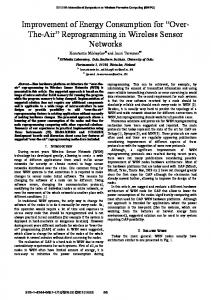
Fig. 6. Deployment of simulation. Blue rings are sensor nodes, the node in the green ring is the user that wants to know the target information. The red ring and line are the starting point and trajectory of the target separately.
the state information, sleep periods from the node who wants to know the target information to the active state nodes are decreasing. So the node sends the query packet along the sleep periods decreasing route to find active state nodes, at the same time it will find the information it needs. Theorem 4: The sleep periods decreasing route has the shortest number of hops from the node who wants to get the information to the target. Proof: When one node wakes up, it updates its state first. If the node is in sleep state, it gets its new number of hops to the target. The node chooses the shortest value from the hops is has received to compute out its sleep period. So the query goes to the target directly. The hops between them is the shortest number of hops. The query walks alone the sleep periods decreasing route, which means it walks alone the hops decreasing route without detour. We can also say the sleep periods decreasing route is the shortest path from the node who wants to get the information to the target. Then we analyze the latency of GQA for the nodes to get the target information theoretical.
Fig. 7.
Sleep periods of every node at initialization phase.
routes are labeled in pink lines. Figure 4(a) is the time slot of initialization, Node 1 can get the target information at every time slot 2nTu (n = 1, 2, 3...), while Node 2 can get the data at every time slot 16nTu (n = 1, 2, 3...). In Fig 4(b) Node 1 and Node 2 can get the information of the target at every time slot 4nTu and 8nTu (n = 1, 2, 3...) separably.
Theorem 5: If the hop between the farthest two nodes has the largest value Hmax . The longest latency for the node to get the target information is 2(Hmax −1) Tu .
V. M ULTI - TARGETS Usually there are more than one target to be monitored in the network, in this situation, our method still works well. In the initialization phase, every node only markets the first received notification and ignores others. In the transformation phase, if one node gets more than one state form different targets, the priority of these three states is {active>listen>sleep}, it chooses the highest priority state it has received. If the node is in sleep state, and receives more than one hop information from different targets, it chooses the smallest one. For example, there are two targets in Fig 5, node 1 (labeled as Node1) gets the listen state from target 1 (labeled as Target1) and hop=2 from target 2 (labeled as Target2), it chooses listen state of target 1, because listen state’s priority is higher than sleep state. Node 2 (labeled as Node2) receives hop=4 from target 1 and hop=2 from target 2, for 2 < 4, then it computes out its sleep period with hop=2 of target 2.
Proof: The node can only get information when it wakes up, so the latency is equal to its sleep period. The longest sleep period is the longest latency. From Theorem 3 we know the longest sleep period is 2(Hmax −1) Tu , which means the longest latency is also 2(Hmax −1) Tu in GQA. The latency of GQA is equal to the sleep period. The maximum latency is 2(Hmax −1) Tu . In the applications of target monitoring, the target information is not necessarily all the time. So this latency could be accepted in these applications. As we can see in Fig 4, nodes in pink rings want to know the target information. The target information always stored in active state nodes, which are labeled as red nodes. Query packets walk along the sleep periods decreasing routes, and reach active state nodes to get the target information, these 106
3.5
100
3
60 40
SSA Synchronous sleep Without sleep
2 1.5 1
20 0 0
x 10
2.5
80
Energy cost
Number of wake up nodes
4
120
0.5 50
100
150 200 Time (s)
250
300
0 0
350
50
100
(a) Fig. 8.
150 200 Time (s)
250
300
350
(b)
Simulation results. (a) number of nodes wake up when the target stationary (b)energy cost when the target stationary.
7
100
6
80
5
Energy cost
Number of wake up nodes
4
x 10
120
60 40
SSA Synchronous sleep Without sleep
4 3 2
20 0 0
1 200
400 Time (s)
0 0
600
(a) Fig. 9.
200
400 Time (s)
600
(b)
Simulation results. (a)number of nodes wake up when the target moving (b)energy cost when the target moving.
The target information is still stored in active state nodes of the target it belongs to. And the query walks along the sleep periods decreasing route to find the target. But it may find the target it does not interested, in this case, it has to find out another route to get the information it needs, the method of [27] could be used here. The sleep periods of nodes could make up ISO-counts, the query packet may find the junction of the two targets, and reach the target it interested through the junction of them.
stay at this position for 350s, the numbers of wake up nodes at every second are in Fig 8(a). We compare the energy cost of SSA to without sleep and synchronous sleep with sleep period equal to Tu in Fig 8(b). To simplify computation we assume the node in sleep state does not cost energy while in all other states costs one slot energy per second. When the target moving, the network turned in to state transformation phase. The numbers of wake up nodes at every second are in Fig 9(a), and the compare results of energy cost of SSA to the schemes of without sleep and synchronous sleep with sleep period equal to Tu are in Fig 9(b). As in Fig 8(b) and Fig 9(b), the energy cost of SSA is much smaller than the schemes of without nodes sleep and all the nodes synchronous sleep with sleep period equal to Tu .
VI. S IMULATION We deployed 100 sensor nodes in a 90*90m2 area, every node can communicate with its one hop neighbors, as shown in Fig 6. The target stayed at position (450,450) which labeled in red ring for 350s, then it moved along the red line with the max , speed of 1m/s for 720s. Use T heorem1 Tu = VmaxD 2(Hmax −1) we can compute out Tu = 5s in this simulation, and we set Tc = 1s. The node at (90,90) labeled in green ring is the user who wants to know the target information. In initialization phase, the target is at (450,450), and every node computes out its sleep period as in Fig 7. When the target
The node at (90,90) labeled in green ring is the user wants to get the target information. It can get information in the initialization phase and state transformation phase when it wakes up. In the state transformation phase, it wakes up at 20s, 40s, 60s, 80s, 100s, 120s, 140s, 160s, 180s, 220s, 260s, 300s, 380s, and 540s. So it can query information at 0s and time slots above. We compare the route length of GQA to Double
107
Number of hops
20
[6] S. Ren, Q. Li, H.N.Wang, X. Chen, and X. Zhang, Probabilistic coverage for object tracking in sensor networks, Mobicom 2004 Poster Session, 2004. [7] C. Gui and P. Mohapatra, Power conservation and quality of surveillance in target tracking sensor networks, ACM Mobicom, 2004. [8] S. Slijepcevic, M. Potkonjak, Power efficient organization ofwireless sensor networks, Preceedings of IEEE International Conference on Communications (ICC01), 2001. [9] Z. Abram, GoelA, S. Plotkin, Set K-cover algorithms for energy efficient monitoring in wireless sensor networks, Proceedings of the 3rd International Conference on Information Processing in SensorNetworks (IPSN04), 2004. [10] C. Liu,K. Wu, V. King, Randomized coverage-preserving schedacling schemes forwireless sensor networks, Preceedings of IFIP Networkong, 2005. [11] F. Ye, G. Zhong, S.Lu, et al, A robust energye on serving protocol for long-lived sensor networks, IEEE Computer Society Press, pages 28-37, 2003. [12] T. Di, G. NicolasD, A coverage-preserving node scheduling scheme for large wireless sensor networks, The 1st ACM international workshop on wireless sensor network and application, 2002. [13] S. Shenker, S. Ratnasamy, B. Karp, R. Govindan, and D. Estrin, Datacentric storage in sensornets, ACM SIGCOMM HotNets, 2002. [14] C. Intanagonwiwat, R. Govindan, and D. Estrin, Directed diffusion: a scalable and robust communication paradigm for sensor networks, MobiCom 2000: Proceedings of the 6th annual international conference on Mobile computing and networking, pages 56-67, 2000. [15] S. Madden, M. J. Franklin, J. M. Hellerstein, and W. Hong, Tag: a tiny aggregation service for ad-hoc sensor networks, Proceedings of the 5th symposium on Operating systems design and implementation, pages 131-146, 2002. [16] S. Ratnasamy, L. Yin, F. Yu, D. Estrin, R. Govindan, B. Karp, and S. Shenker, GHT: A geographic hash table for datacentric storage in sensornets, Proc. of the 1st ACM International Workshop on Wireless Sensor Networks and Applications (WSNA), pages 78-87, September 2002. [17] S. Funke, L. Guibas, A. Nguyen, and Y. Wang, Distance-sensitive routing and information brokerage in sensor networks, DCOSS 2006, pp. 234-251, 2006. [18] J. Li, J. Jannotti, D. Decouto, D. Karger, and R. Morris, A scalable location service for geographic ad-hoc routing, Proceedings of 6th ACM/IEEE International Conference on Mobile Computing and Networking, pages 120-130, 2000. [19] X. Li, Y. J. Kim, R. Govindan, and W. Hong, Multi-dimensional range queries in sensor networks, Proceedings of the first international conference on Embedded networked sensor systems, pages 63-75, 2003. [20] R. Sarkar, X. Zhu, J. Gao, Double Rulings for Information Brokerage in Sensor Networks, MobiCom06, 2006. [21] M. Chu, H. Haussecker, and F. Zhao, Scalable informationdriven sensor querying and routing for ad hoc heterogeneous sensor networks, Int’l High Performance Computing Applications, 16(3):90-110, 2002. [22] J. Faruque and A. Helmy, UGGED: Routing on fingerprint gradients in sensor networks, IEEE Int’l Conf. on Pervasive Services (ICPS), pages 179-188, July 2004. [23] J. Faruque, K. Psounis, and A. Helmy, Analysis of gradientbased routing protocols in sensor networks, IEEE/ACM Int’l Conference on Distributed Computing in Sensor Systems (DCOSS), pages 258-275, June 2005. [24] J. Liu, F. Zhao, and D. Petrovic, Information-directed routing in ad hoc sensor networks, IEEE Journal on Selected Areas in Communications, 23(4):851-861, April 2005. [25] F. Ye, G. Zhong, S. Lu, and L. Zhang, GRAdient broadcast:A robust data delivery protocol for large scale sensor networks, ACM Wireless Networks (WINET), 11(3):285-298, 2005. [26] H. Lin, M. Lu, N. Milosavljevic, J. Gao, L. J. Guibas, Composable Information Gradients in Wireless Sensor Networks, International Conference on Information Processing in Sensor Networks (IPSN 2008), pages 121132, 2008. [27] R. Sarkar, X. Zhu, J. Gao, L. J. Guibas, J. S. B. Mitchell, Iso-Contour Queries and Gradient Descent with Guaranteed Delivery in Sensor Networks, Proc. of the 27th Annual IEEE Conference on Computer Communications (INFOCOM’08), May, 2008.
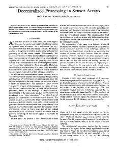
GQA Double rulings
15
10
5
0
0 2 4 6 8 10 12 14 16 18 22 26 30 38 54
Time (10s) Fig. 10.
Number of hops needed for the query reaches the target.
Rulings [20] in Fig 10. The hops of GQA shorter than Double Rulings, which means it costs less energy in query phase. But GQA brings larger latency than Double Rulings, as GQA focuses on the applications of target monitoring, which the target information is not necessarily all the time. The latency of GQA is no longer than 2(Hmax −1) Tu , and this latency could be accepted in these applications. VII. C ONCLUSION For energy constrained wireless sensor networks, duty cycling is an effective technique to prolong the lifetime of the network. Previous duty cycling mechanisms keep the assumptions of fully covering the deployment area, which is not necessary for certain applications like target monitoring. In this paper, we propose the novel duty cycle design for the sensor networks of target monitoring, which can prolong the lifetime of the network as far as possible, and can answer the target information queries through gradient query routing. Both the analytical and experimental results prove the functionality of the proposed design on the reduction of energy consumption. ACKNOWLEDGMENT This work is supported in part by the National High Technology Research and Development Program of China (863 Program) under grant No.2006AA09Z113, the National Basic Research Program of China (973 Program) under grant No. 2006CB303000, NSF China grant No. 60703082. R EFERENCES [1] Q Cao, T Abdelzaher, T He, J Stankovic, Towards optimal sleep scheduling in sensor networks for rare-event detection, Proceedings of the 4th international symposium on Information processing in sensor networks, 2005. [2] X. Wang, et al., Integrated coverage and connectivity configuration in wireless sensor networks, ACM SenSys, 2003. [3] T. Yan, T. He, and J. A. Stankovic, Differentiated surveillance for sensor networks, ACM SenSys, 2003. [4] D. Tian and N.D.Georganas, A node scheduling scheme for energy conservation in large wireless sensor networks, Wireless Communications and Mobile Computing Journal, 2003. [5] T. He, S.Krishnamurthy, J. A. Stankovic, T. Abdelzaher, L. Luo, R. Stoleru, T. Yan, L. Gu, G. Zhou, J. Hui, and B. Krogh, Vigilnet:an integrated sensor network system for energy-efficient surveillance, ACM Transaction on Sensor Networks, 2006.
108