Smooth Invariant Interpolation of Rotations F. C. PARK Seoul National University and BAHRAM RAVANI University of California, Davis
We present an algorithm for generating a twice-differentiable curve on the rotation group SO(3) that interpolates a given ordered set of rotation matrices at their specified knot times. In our approach we regard SO(3) as a Lie group with a bi-invariant Riemannian metric, and apply the coordinate-invariant methods of Riemannian geometry. The resulting rotation curve is easy to compute, invariant with respect to fixed and moving reference frames, and also approximately minimizes angular acceleration. Categories and Subject Descriptors: I.3.7 [Computer Graphics]: Three-Dimensional Graphics and Realism—animation, geometric algorithms General Terms: Algorithms, Theory Additional Key Words and Phrases: Cubic spline, interpolation, Lie algebra, Lie group, mathematics, rotation
1. INTRODUCTION A common problem that arises not only in computer graphics and animation, but also in applications ranging from robot motion planning to machine vision, is the interpolation of smooth curves on the rotation group, also known as the Special Orthogonal Group SO(3). In this article we address the following problem: given an ordered set of n 1 1 rotation matrices {R0, R1, . . . , Rn }, and a set of n 1 1 scalars t 0 , t 1 , . . . , t n , This work was supported in part by US Army Research Office grant number DAAL03-90-G0005 and in part by the California Department of Transportation through the AHMCT program. F. C. Park was also supported in part by the Engineering Research Center for Advanced Control and Instrumentation at Seoul National University. Authors’ addresses: F. C. Park, Department of Mechanical Design and Production Engineering, Seoul National University, Seoul, Korea; B. Ravani, Department of Mechanical and Aeronautical Engineering, University of California, Davis, Davis, CA 95616; email: ^
[email protected]&. Permission to make digital / hard copy of part or all of this work for personal or classroom use is granted without fee provided that the copies are not made or distributed for profit or commercial advantage, the copyright notice, the title of the publication, and its date appear, and notice is given that copying is by permission of the ACM, Inc. To copy otherwise, to republish, to post on servers, or to redistribute to lists, requires prior specific permission and / or a fee. © 1997 ACM 0730-0301/97/0700 –0277 $03.50 ACM Transactions on Graphics, Vol. 16, No. 3, July 1997, Pages 277–295.
278
•
F. C. Park and B. Ravani
find a twice-differentiable curve R(t) on the rotation group such that R(t i ) 5 Ri , i 5 0, 1, . . . , n. Our goal is to find a fast, reference frame-invariant method of interpolating smooth curves on the rotation group. Although well-established methods exist for interpolation in finite-dimensional vector spaces, the majority of these techniques do not easily generalize in a uniform and coordinate-invariant way to curved spaces such as the rotation group. Some recent work toward this end includes that of Brunnett and Crouch [1994], Noakes et al. [1989], and Zefran et al. [1995]. In Brunnett and Crouch [1994], a detailed variational analysis of minimum acceleration curves on the sphere is given, whereas in Noakes et al. [1989] and Zefran et al. [1995] the variational equations are derived for minimum acceleration curves on Riemannian manifolds and the Lie group of rigid body motions, respectively. The focus of these variational analyses is on obtaining qualitative results rather than computational algorithms; in general their solutions require the integration of nonlinear differential equations with split boundary conditions, which severely limits their practicality for CAD applications. Because of its practical importance the problem of interpolation on the rotation group has received much attention in the literature. Most of the existing work involves choosing some local coordinate parametrization for rotations (e.g., Euler angles or unit quaternions) and applying existing vector space spline algorithms to these local coordinates. Although computationally efficient, one obvious drawback to such approaches is that, unlike the variational methods previously mentioned, the resulting curve typically will depend on the choice of local coordinates. When the underlying space is curved, often the price for coordinate-invariance is a substantial increase in the amount of computation. Interactive curve design, on the other hand, demands speed as well as accuracy, and in such situations the practical solution is usually a compromise between the efficiency offered by coordinate-based approaches, and the physical and mathematical consistency offered by purely intrinsic approaches. It is therefore important to understand how the choice of coordinates affects the behavior of the curve vis-a´-vis the intrinsic solution. In the case of rotations, another equally important issue is the question of bi-invariance. Given two ordered sets of rotation matrices {R0, . . . , Rn } # 0, . . . , R # n }, related by R # i 5 PRi Q, i 5 0, 1, . . . , n for a pair of and {R constant rotation matrices P and Q, it is reasonable to demand that the # (t), respecinterpolating curves through these two sets, denoted R(t) and R # tively, be related by R(t) 5 PR(t)Q. Physically this relation reflects the fact that the orientation component of the interpolated motion for a rigid body moving in space should not be influenced by the choice of fixed (i.e., global) or moving (i.e., attached to the moving body) reference frames. In this article we present an algorithm for interpolating twice-differentiable bi-invariant trajectories on the rotation group. The resulting trajectory approximately minimizes angular acceleration in the same sense that cubic splines can be viewed as approximations to minimum curvature ACM Transactions on Graphics, Vol. 16, No. 3, July 1997.
Interpolation of Rotations
•
279
curves. The key ingredients of the algorithm are obtained by specializing standard concepts from the theory of Lie groups to SO(3), which can also be regarded as a Lie group with a bi-invariant Riemannian metric. In particular, the canonical coordinates of the first kind act as a natural set of local coordinates on SO(3), and the exponential map leads to a simple geometric visualization of the rotation group. The article is organized as follows. In Section 2 we present in the context of SO(3) the basic concepts of matrix Lie groups. We also discuss the Lie group structure of the Special Unitary Group SU(2), which can in turn be identified with the unit quaternions. In Section 3 we review the variational equations for a minimum angular acceleration curve that interpolates two given rotations, and show that if the rotations are “sufficiently close,” then the solution is given by the exponential of a certain cubic matrix polynomial. This curve moreover is shown to be bi-invariant, independent of the closeness assumption, and in several special but important cases coincides with the minimum angular acceleration curve. In Section 4 the two-point interpolation results of the previous section are extended to a multiplepoint interpolation algorithm. We conclude in Section 5 with some remarks on the interpolation of general rigid body motions. Before proceeding we mention some of the relevant previous work in SO(3) interpolation. One of the more widely cited approaches is the work of Shoemake [1985], who presents a class of interpolation schemes based on the unit quaternion representation for rotations. Part of the appeal behind the unit quaternions is that they provide a globally nonsingular fourparameter representation for rotations. As we explain later in more detail, it is important to keep in mind that the unit quaternions, or equivalently SU(2), are not the same as SO(3), but rather a double covering. This latter fact is often overlooked in many quaternion-based approaches, which sometimes leads to wildly spinning trajectories. Even with a proper accounting of this fact the resulting algorithms can often become cumbersome. Shoemake’s algorithm can essentially be viewed as a generalization of De Casteljau’s construction for Be´zier curves to SU(2), in which straight lines are now replaced by minimal geodesics. This algorithm, although producing intrinsic curves, has the expected disadvantage of high computational cost, as well as the additional bookkeeping required because of the doublecovering property. Also, some of the standard properties possessed by Be´zier curves in Euclidean space are not preserved in Shoemake’s formulation. In Park and Ravani [1995] we argue that the present circle of geometric ideas can be used to formulate a more elegant and compact construction of Be´zier curves in SO(3) (and other Lie groups) much more succinctly. A more careful geometric analysis of unit quaternion-based methods is given by Ge and Ravani [1994a,b], in which the underlying curved geometry is considered in performing the interpolation, and a proper analysis and evaluation of the characteristics of the resulting Be´zier representations are given. Kim and Nam [1996] also propose a unit quaternion-based method of ACM Transactions on Graphics, Vol. 16, No. 3, July 1997.
280
•
F. C. Park and B. Ravani
generating Hermite interpolants on SO(3) that uses circular blending arcs. Juttler and Wagner [1994; 1996] consider the generation of rigid-body motions using dual quaternion curves, and discuss the issues associated with the dependence of the existing methods on the coordinate system used. Hart et al. [1994] have presented an interesting method for visualization of quaternion curves that represent three-dimensional rotations, and Barr et al. [1992] also present an interpolation algorithm based on quaternions that handles angular velocity constraints.
2. THE GEOMETRY OF SO(3) We begin with a review of the necessary background on SO(3) as a matrix Lie group; the development closely parallels that of Park and Ravani [1995], and additional background can be found, for example, in Belinfante and Kolman [1972]. We close this section with a brief discussion of the Lie group structure of the Special Unitary Group SU(2), which can be identified with the unit quaternions. 2.1 SO(3) as a Lie Group Before reviewing the Lie group structure of SO(3), it is instructive to consider the simplest nontrivial Lie group, the unit circle S1, as a motivating example. Clearly S1 forms a smooth one-dimensional space, or a manifold of dimension one. Points in S1 can be parametrized in the complex plane as z 5 cos u 1 i sin u for 0 # u # 2p. Multiplying two points in S1 results in another point in S1; in fact, it is not difficult to see that S1 forms an algebraic group under complex multiplication. Another way to display this group structure is to arrange an element of S1 as the 2 3 2 rotation matrix
F
cos u 2sin u sin u cos u
G
.
(1)
The set of such matrices forms the algebraic group SO(2) under matrix multiplication. The final observation is that an element of S1 can be written as the exponential e i u 5 cos u 1 i sin u 5 z, or in matrix form as
F
cos u 2sin u sin u cos u
G
5 exp
F
0 2u u 0
G
.
(2)
where exp( z ) here denotes the matrix exponential (defined in the following). In both the scalar and matrix representations the exponential map provides a natural means of parametrizing the circle S1 by a single coordinate u. As previously shown, the circle S1 is equivalent to the 2 3 2 rotation matrices SO(2). This set has the structure of both an algebraic group and differentiable manifold, and is an example of a Lie group. The rotation ACM Transactions on Graphics, Vol. 16, No. 3, July 1997.
Interpolation of Rotations
•
281
group SO(3) is the set of all 3 3 3 real orthogonal matrices with unit determinant. It is not difficult to see that SO(3) will also have the structure of a group (under matrix multiplication) and a differentiable manifold, or a Lie group. Some other well-known examples of Lie groups include the rigid-body motions SE(3), whose elements admit the 4 3 4 matrix representation
F
R b 0 1
G
,
(3)
where R [ SO(3) and b [ R3; Gl(n), the general linear group of n 3 n real nonsingular matrices, and the special linear group Sl(n), which is a subgroup of Gl(n) whose elements have unit determinant. Let A be a point on a matrix Lie group &, and X(t) be any differentiable curve on & that passes through A at t 5 0; that is, X(0) 5 A. The derivative ˙ (0) is said to be a tangent vector to & at A; the set of all tangent vectors at X A, denoted TA&, forms a vector space, called the tangent space to & at A. The tangent space at the identity A 5 I is given a special name, the Lie algebra of &, and is denoted by the lowercase g. On SO(3) it is easily shown that the Lie algebra so(3) consists of the 3 3 3 skew-symmetric matrices: if R(t) is a curve in SO(3) such that R(0) 5 I, then differentiating both sides ˙ T(0) 1 R ˙ (0) 5 0, so that elements of so(3) of RT(t)R(t) 5 I, it follows that R are matrices of the form
@r#–
3
0 2r 3 r 2 r3 0 2r 1 2r 2 r 1 0
4
,
(4)
where r [ R3. Note that an element [r] [ so(3) can also be represented as a vector r [ R3. More generally a Lie algebra is a vector space 9, together with a bilinear map [ z , z ]: 9 3 9 3 9 (called the Lie bracket) that satisfies, for every h, m, j [ 9, (i) [h, h] 5 0, and (ii) [h, [m, j]] 1 [j, [h, m]] 1 [m, [j, h]] 5 0. From (i) and the bilinearity property it follows that [h, m] 5 2[m, h]. For matrix Lie groups and Lie algebras the corresponding Lie bracket reduces to the standard matrix commutator: if h and m are square matrices, then [h, m] 5 hm 2 mh. In particular, on so(3) it is easily verified that the Lie bracket of two elements corresponds to their vector product: [r1, r2] 5 [r1][r2] 2 [r2][r1] 5 [r1 3 r2]. One final notion that combines elements of both a Lie group and its Lie algebra is the adjoint map. If X and x are, respectively, arbitrary elements of a matrix Lie group and its Lie algebra, then XxX21 is another element of the Lie algebra. On SO(3) the following identity can be established: if R [ SO(3) and r [ so(3), then R[r]RT 5 [Rr]. We make frequent use of this identity later. ACM Transactions on Graphics, Vol. 16, No. 3, July 1997.
282
•
F. C. Park and B. Ravani
2.2 The Exponential Map One of the main connections between a Lie group and its Lie algebra is the exponential mapping; defined on each Lie algebra is the exponential mapping into the corresponding Lie group. On matrix groups the exponential mapping is given by the usual matrix exponential, that is, if A is an element of the Lie algebra, then eA 5 I 1 A 1 (A2/2!) 1 . . . is an element of the Lie group. On so(3) the exponential mapping is onto; that is, for every R [ SO(3) there exists at least one [r] [ so(3) such that e[r] 5 R. On SO(3) and its Lie algebra well-known closed-form formulas exist for the exponential and its inverse. If [r] [ so(3), then
e @r # 5 I 1
sin iri iri
z @r# 1
1 2 cos iri iri 2
z @ r # 2,
(5)
where iri is the standard Euclidean norm. Conversely, if R [ SO(3) such that Tr(R) Þ 21, then
log R 5
f 2 sin f
~ R 2 R T! ,
(6)
where f satisfies 1 1 2 cos f 5 Tr(R) and ilog Ri2 5 f2. If we restrict f to be between 0 and p, then in the case when Tr(R) 5 21, two solutions for log R exist: if vˆ is a unit length eigenvector of R associated with the eigenvalue 1, then log R 5 6p[vˆ]. The coordinates r can in fact be identified with the canonical coordinates of the first kind for the Lie group SO(3) [Chevalley (1946)]. On general Lie groups these canonical coordinates provide a natural local parametrization about a neighborhood of the identity. In the case of SO(3) this neighborhood covers all of SO(3) except for a “thin” set. To visualize this parametrization, first recall that every arbitrary rotation can be represented by a rotation about some fixed axis in space passing through the origin. SO(3) can therefore be geometrically pictured as a three-dimensional solid ball of radius p, centered at the origin, with the antipodal points identified: a point r in the ball represents a rotation by iri radians (in the right-hand sense) about the line directed from the origin through r. The exponential and logarithm give explicit formulas for this solid ball representation of SO(3). Some remarks are in order. First, this representation is unique only when restricted to the interior of the solid ball, as antipodal points on the boundary of the solid ball clearly correspond to the same physical rotation. Second, because of the 2p periodicity of rotations, it follows that if [r] is one solution to log R, then so is [r](1 1 (2 p k/iri) for any integer k. 2.3 Angular Velocities and so(3) The Lie algebra so(3) provides a set of local coordinates for SO(3) via the exponential map. Another important connection between so(3) and SO(3) ACM Transactions on Graphics, Vol. 16, No. 3, July 1997.
Interpolation of Rotations
•
283
involves angular velocities. If R(t) is a curve in SO(3) describing the orientation of a rigid body relative to a fixed reference frame, then a simple ˙ RT and RTR ˙ are skew-symmetric, and hence calculation reveals that both R T˙ elements of so(3). R R is in fact the angular velocity of the rigid body ˙ RT is the angular velocexpressed in moving-frame coordinates, whereas R ity expressed in fixed-frame coordinates. The angular acceleration vector with respect to either the fixed or moving frame is then obtained by differentiating the appropriate angular velocity representation. The application to SO(3) of the following formula, which is valid for general matrix Lie groups, is one of the key steps in the derivation of our interpolation algorithm. Let x(t) be a curve on a matrix Lie algebra, and X(t) 5 ex(t) be a curve on the corresponding matrix Lie group. Then it can be shown that
˙ 5 X 21X
E
1
e 2x~t!sx˙ ~ t ! e x~t!sds
(7)
e x~t!sx˙ ~ t ! e 2x~t!sds.
(8)
0
and
˙ X 21 5 X
E
1
0
If [r(t)] 5 x(t) is a curve on so(3) and R(t) 5 e[r(t)] is the corresponding curve on SO(3), then by explicitly evaluating the integral in the preceding formula a closed-form expression for the angular velocity can be obtained in terms of the canonical coordinates x. First, denote by vb (t) the angular ˙. velocity with respect to the moving (body) frame; that is, [vb (t)] 5 RTR Then
v b~ t ! 5 A ~ r ! r˙ ,
(9)
where
A~r! 5 I 2
1 2 cosiri iri
2
@r# 1
iri 2 siniri iri 3
@ r # 2.
(10)
Similarly, the angular velocity with respect to the fixed frame, denoted vs (t), is given by vs (t) 5 B(r)r˙, with
B~r! 5 I 1
1 2 cosiri iri
2
@r# 1
iri 2 siniri iri 3
@ r # 2.
(11)
It can be verified that both A and B are nonsingular for all r. ACM Transactions on Graphics, Vol. 16, No. 3, July 1997.
284
•
F. C. Park and B. Ravani
2.4 Lie Group Structure of SU(2) In this section we discuss the Lie group structure of the Special Unitary Group SU(2), and demonstrate its equivalence with the unit quaternions. Although these results have been known in the mathematics and physics community, the formulas we establish here are either scattered throughout the literature or appear not to have been explicitly derived. SU(2) is defined to be the set of 2 3 2 complex unitary matrices with unit determinant: any M [ SU(2) satisfies M*M 5 MM* 5 I and detM 5 1, where M* denotes the complex conjugate transpose of M. From the definition it follows that M is of the form
M5
F
a b 2 b# a#
G
,
(12)
where . denotes complex conjugation. If a 5 q 0 1 iq 1 and b 5 q 2 1 iq 3 , then from the definition we must have q 20 1 q 21 1 q 22 1 q 23 5 1. Hence SU(2) can be identified with the unit 3-sphere in R4, which is clearly a differentiable manifold. That SU(2) forms an algebraic group (under matrix multiplication), and hence a Lie group, can also be easily verified. The identification with the unit quaternions can be made by writing M [ SU(2) as q 0 1 q 1 i 1 q 2 j 1 q 3 k. As seen from the foregoing, the rather unintuitive rule for quaternion multiplication turns out to be simply group multiplication in SU(2). Following our derivation of the Lie algebra so(3), the Lie algebra of SU(2), denoted by the lower-case su(2), can be shown to consist of all complex 2 3 2 skew-Hermitian matrices with trace zero. More specifically, an element of su(2) has the form iA, where
A5
F
x1 x 2 1 ix 3 x 2 2 ix 3 2x 1
G
.
(13)
The Lie bracket on su(2) is also given by the matrix commutator: [iA, iB] 5 BA 2 AB. A simple calculation shows that the Lie bracket on su(2) can also be interpreted as the cross-product in R3. The corresponding exponential and logarithm maps for SU(2) are given by the following formulas:
exp ~ iA ! 5 I cosiAi 1 i
log ~ M ! 5
f/ 2 2 sin f / 2
A iAi
siniAi
~ M 2 M* ! ,
(14)
(15)
where iAi 5 ( x 21 1 x 22 1 x 23 ) 1/ 2 . These two formulas define the canonical coordinates for SU(2). As alluded to earlier, there exists a 2–1 group homomorphism (i.e., a mapping which preserves group operations) between SU(2) and SO(3), so ACM Transactions on Graphics, Vol. 16, No. 3, July 1997.
Interpolation of Rotations
•
285
that SU(2) can be regarded as a double covering of SO(3). This mapping can be obtained as follows. Given R [ SO(3), suppose log R 5 [v ˆ ]f, where v ˆ [ R3 is of unit length and 0 # f # p; R is thus a rotation about the axis v ˆ by an angle of f radians. The two elements in SU(2) corresponding to R are then (q 0 , q 1 , q 2 , q 3 ) 5 (cos (f/2), v1 sin (f/2), v2 sin (f/2), v3 sin (f/2)) and (q 0 , q 1 , q 2 , q 3 ) 5 (2cos (f/2), 2v1 sin (f/2), 2v2 sin (f/2), 2v3 sin (f/2)). Thus antipodal points in SU(2) correspond to the same rotation in SO(3).
3. TWO-POINT INTERPOLATION 3.1 Minimum Angular Acceleration Curves In this section we formulate, in a purely matrix setting, the variational problem of determining minimum angular acceleration curves in SO(3). From physical reasons it should be apparent that the solution must be coordinate-invariant. It turns out that in a few limited but interesting cases an analytic solution to this variational problem can be found; we review both these solutions as well as the precise form of the general Euler-Lagrange equations. In what follows we choose to represent the angular acceleration in terms of the moving frame coordinates, although this choice is completely arbitrary. The angular velocity in moving frame coordinates is given by [v] 5 ˙ . Rewriting this equation as R ˙ 5 R[v], the variational formulation of R TR the minimum angular acceleration problem is as follows: find a curve R(t) in SO(3) that minimizes
E
1
v ˙ Tv ˙ dt
(16)
0
˙ 5 R[v], with R(0) 5 R0, R(1) 5 R1, v(0) 5 v0, and v(1) 5 v1 subject to R given as boundary conditions. The corresponding Euler-Lagrange equations are
d 3v dt 3
1v3v ¨ 5 0.
(17)
This equation, although deceptively simple in appearance, does not admit a general closed-form solution. However, in the following three special cases a closed-form solution can be found. First, if v(0) 5 v(1) Þ 0, then the solution is given by
R ~ t ! 5 R 0e @r #t,
(18)
where r 5 log(RT 0 R1). In this case R(t) is the minimum energy solution; that is, it minimizes *10 vTvdt. The second special case is when v(0) 5 v(1) ACM Transactions on Graphics, Vol. 16, No. 3, July 1997.
286
F. C. Park and B. Ravani
•
5 0; in this case the solution is given by 2
3
R ~ t ! 5 R 0e @r#~3t 22t !.
(19)
See Zefran et al. [1995] for a proof of the preceding two cases. The final special case is when v(0) 5 v ˙ (0) 5 0, in which case the solution to the Euler-Lagrange equations is
R ~ t ! 5 e @r #t
3
(20)
as can be easily verified by using Equation (7). This is a particularly important case, as it corresponds to the popular natural spline in curve design (see the following). In all these cases the solution is a rotation about the axis fixed in the direction of r. One can verify that these expressions for R(t) are indeed solutions by substituting them into the Euler-Lagrange equations. In general, however, closed-form expressions for minimum angular acceleration curves are extremely difficult to find, so that one must resort to time-consuming and computationally expensive numerical methods to determine the solution. 3.2 Cubic Interpolation Solving the preceding two-point boundary value problem numerically clearly is not a practical option for interactive CAD applications. However, if the two rotations are assumed “close” to one another (in a sense to be made precise in the following section), then by employing the canonical coordinates one can obtain a suboptimal “cubic” solution. The argument employed here is quite similar in spirit to the standard one given for approximating minimum energy splines, or elastica, by cubic polynomials: if the second derivative of the curve is not too large, then the squared norm of the second derivative provides a reasonable approximation to the elastic energy, and the corresponding solution will be a cubic polynomial. The solution on SO(3) that we obtain has the further desirable property of being bi-invariant. In this section we derive this particular cubic interpolant on SO(3). By differentiating the angular velocity vector vb (t) of Equations (9) and (10), one obtains the angular acceleration vector a(t) relative to the moving frame, expressed in terms of the canonical coordinates. Following a somewhat lengthy calculation, the angular acceleration vector is given as follows:
a ~ t ! 5 r¨ 2 1 1
r Tr˙ iri
r Tr˙ iri 5
4
~ 2 cos i r i 1 i r i sin i r i 2 2 !~ r 3 r˙ ! 2
1 2 cosiri iri 2
~ r 3 r¨ !
~ 3 sin i r i 2 i r i cos i r i 2 2 i r i!~ r 3 ~ r 3 r˙ !!
iri 2 siniri iri 3
~ r˙ 3 ~ r 3 r˙ ! 1 r 3 ~ r 3 r¨ !! .
ACM Transactions on Graphics, Vol. 16, No. 3, July 1997.
(21)
Interpolation of Rotations
•
287
Here i z i denotes the Euclidean norm in R3. Having expressed everything in terms of canonical coordinates, the variational problem now reduces to finding the curve r(t) [ R3 that minimizes *10 ia(t)i 2 dt subject to r(0) 5 0, r˙(0) 5 A21(r0)v0, r(1) 5 r1 with [r1] 5 log(RT ˙ (1) 5 A21(r1)v1, 0 R1), and r with A given by Equation (10). The solution R(t) is then given by
R ~ t ! 5 R 0e @r~t!#.
(22)
If R0 is close to R1 in the sense that RT 0 R1 is close to I, then the boundary condition on r(1) is approximately r(1) 5 0. If in addition the initial and final angular velocities are not too large, then the solution r(t) can also be expected to remain small. Under this assumption the angular acceleration vector a(t) is approximately r¨(t); the solution curve in this case is given by the cubic polynomial
r ~ t ! 5 at 3 1 bt 2 1 ct,
(23)
where a, b, c [ R3 are constant vectors satisfying (i) a 1 b 1 c 5 r1; (ii) c 5 v0; (iii) 3a 1 2b 1 c 5 A21 (r1)v1. The resulting solution curve in SO(3) is then given by 3
2
R ~ t ! 5 R 0e @at 1bt 1ct#.
(24)
In the Appendix we show that the cubic solution (24) is bi-invariant. It should be apparent from physical considerations alone that the minimum angular acceleration curve—that is, the solution to the original variational problem—must necessarily be bi-invariant. 3.3 Accuracy of the Cubic Approximation Because SO(3) is a curved space, establishing sharp bounds on the accuracy of the cubic approximation to the minimum angular acceleration curve turns out to be a difficult problem. Standard results from function approximation theory, which are usually formulated in a Hilbert space setting, cannot be directly applied to this situation. In fact, even the basic question of how to measure the distance between two elements of SO(3), which is fundamental to formulating any notion of error, needs to be addressed. In this section we try to gain some insight into how well-behaved the cubic approximation is as the endpoint rotations become more “distant” from each other. To begin, observe that for the three special cases in which a closed-form analytic solution can be found (i.e., when the initial and final angular velocities are both zero, when they are equal and nonzero, and when the initial angular velocity and acceleration are zero), the cubic interpolant is the exact solution to the variational problem. As mentioned earlier, the last case is also quite meaningful from a CAD perspective, as these particular ACM Transactions on Graphics, Vol. 16, No. 3, July 1997.
288
•
F. C. Park and B. Ravani
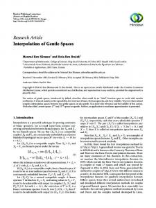
initial conditions correspond to the popular natural spline. Clearly the preceding is a necessary condition for any reasonable approximation scheme. To discuss the approximation accuracy for the remaining cases, a notion of how to measure distance between two rotations is required. Here we give a brief review of some of the results established in Park [1995], where a natural distance metric on SO(3) is derived using our earlier geometric framework. The natural way to define distance between two points on a surface is as the length of the shortest curve connecting them; the length of this minimal geodesic curve is computed by an integral involving the first fundamental form of the surface and a local coordinate parametrization of the curve. Generalizing these concepts to multidimensional surfaces, the surface now becomes a Riemannian manifold, and the first fundamental form the Riemannian metric. Usually one cannot hope to find a “natural” Riemannian metric for a given manifold, in the sense that the metric is determined by the geometry of the underlying space. However, on topologically compact Lie groups such as SO(3) there does exist a natural metric determined by the requirement of bi-invariance. We refer the reader to Park [1995] and any standard text on Riemannian geometry and Lie groups for the mathematical details. The key result for our purposes is that the minimal geodesic connecting two rotations R0 and R1, where length is measured relative to the bi-invariant Riemannian metric, is given by R(t) 5 R0e[r]t , where [r] 5 log(RT 0 R1). The length of the minimal geodesic is simply given by the Euclidean length iri or, equivalently, the amount of rotation (in radians) about r.1 Figure 1 shows the deviation over 0 # t # 1 of the cubic approximation from the optimal curve as a function of time. The optimal curve was determined numerically by the shooting method. Here the deviation is measured using the natural distance metric on SO(3), whose maximum value cannot exceed p. The boundary conditions used for this set of data are
log ~ R 0! 5 ~ 0.2
0.1
0.1 !
(25)
log ~ R 1! 5 ~ 0.6
0.4
0.4 ! .
(26)
The smaller of the two graphs depicts the error function for initial angular velocity v0 5 (0.5, 0.1, 0.1) and initial angular acceleration a0 5 (0.5, 0.1, 0.1). The larger graph corresponds to the initial values v0 5 (5, 1, 1) and a0 5 (0.5, 0.1, 0.1). Figure 2 shows how the interpolated trajectory deviates from the minimum angular acceleration trajectory as a function of the initial and final
1
It is now straightforward to formulate Be´zier curves in SO(3), by simply replacing the straight lines in De Casteljau’s algorithm with minimal geodesics; see Park and Ravani [1995] for details.
ACM Transactions on Graphics, Vol. 16, No. 3, July 1997.
Interpolation of Rotations
•
289
Fig. 1. A plot of deviation versus time for two interpolated trajectories. The smaller graph represents the natural distance between the cubic interpolant and the optimal (i.e., minimum angular acceleration) trajectory for small initial angular velocity and acceleration, and the larger graph depicts the deviation as the initial values are increased five-fold.
orientations. The initial conditions are
R0 5 I
v0 5 ~p
0
0!
a0 5 ~0
0
0!,
and the final orientation is expressed as a function of the parameter p, 0 # p # p:
R 1 5 exp
13
0 0 0 0 0 2p 0 p 0
42
p .
(27)
Note that when p 5 0, both the interpolated trajectory and the minimum angular acceleration curve reduce to the minimal geodesic. As p increases, both the interpolated and minimum acceleration trajectories are forced to deviate from the minimal geodesic. If we denote the minimum angular ˆ (t), then acceleration trajectory by R(t) and the interpolated trajectory by R for a given boundary value R1 the error is measured according to
Error 5
E
1
ˆ i 2dt. ilog ~ R TR
(28)
0
ACM Transactions on Graphics, Vol. 16, No. 3, July 1997.
290
•
F. C. Park and B. Ravani
Fig. 2. A plot of average error as a function of the final orientation R1, which is parametrized by a scalar parameter p.
The resulting graph is symmetric about p 5 p, and therefore we plot only the error values for the range p [ [0, p]. These empirical results give an indication of how the approximation degrades as a function of the boundary conditions. 4. INTERPOLATION OF MULTIPLE POINTS We now present a complete algorithm for interpolating through multiple points in SO(3) using cubic splines. Analogous to the Euclidean case, the interpolated curve in SO(3) maintains continuity of both angular velocities and accelerations at the knot points. The particular version of the algorithm that we present requires the following as inputs: an ordered set of n 1 1 rotation matrices {R0, R1, . . . , Rn} (the knot points), a set of n 1 1 scalars t0 , t1 , . . . , tn (the knot times), an initial angular velocity v0 [ R3, and an initial angular acceleration a0 [ R3. Both v0 and a0 are expressed in moving frame coordinates. i z i here refers to the Euclidean norm. Given:
$ R 0 , R 1 , . . . , R n% 5 knot points $ t 0 , t 1 , . . . , t n% 5 knot times
v 0 5 angular velocity at t 0 in moving frame coordinates a 0 5 angular acceleration at t 0 in moving frame coordinates T ~ Condition: Tr ~ R i21 R i! Þ 21 for i 5 1, 2, . . . , n. !
ACM Transactions on Graphics, Vol. 16, No. 3, July 1997.
Interpolation of Rotations
•
291
Preprocessing: for i 5 1 to n do T @ r i# 5 log ~ R i21 R i!
Ai 5 I 2
1 2 cosir ii ir ii
2
@ r i# 1
ir ii2sinir ii ir ii 3
@ r i# 2
Initialization:
c1 5 v0 b 1 5 a 0/ 2 a1 5 r1 2 b1 2 c1 Iteration: for i 5 2 to n do
s 5 r i ~ temporary variable ! . t 5 3a i21 1 2b i21 1 c i21 ~ temporary variable ! u 5 6a i21 1 2b i21 ~ temporary variable ! c i 5 Ai21ci21 . bi 5
1 2
S
1
1
u2
s Tt isi 5
sTt isi
4
~2 cosisi 1 isisinisi 2 2!~s 3 t! 2
1 2 cosisi isi2
~s 3 u!
~ 3 sin i s i 2 i s i cos i s i 22 i s i!~ s 3 ~ s 3 t !!
isi2sinisi isi 3
~ t 3 ~ s 3 t ! 1 s 3 ~ s 3 u !! ).
ai 5 s 2 bi 2 ci Result: for t i21 # t # t i ,
t5
t 2 t i21 t i 2 t i21 3
2
R ~ t ! 5 R i21e @ait 1bit 1cit#. Formulas for the matrix exponential and logarithm are given by Equations (5) and (6), respectively. ACM Transactions on Graphics, Vol. 16, No. 3, July 1997.
292
•
F. C. Park and B. Ravani
Fig. 3. Top row: 4 knot points; middle row: the cubic interpolant; bottom row: minimum angular acceleration interpolant.
Specifying the initial angular velocity and acceleration as inputs leads to the preceding version of the algorithm. In particular, specifying both these quantities to zero is a popular choice in many applications; in the spline literature such interpolating curves are called natural cubic splines. For other choices of input, for example, specifying the initial and final angular velocities (the so-called clamped spline), the formulas in the algorithm will in general become more complicated. To illustrate why, it is instructive to consider the case of clamped cubic splines in Euclidean space. Recall that determining the polynomial coefficients requires the solution of a tridiagonal linear system, which arises because the coefficients (ai , bi , ci ) are linear functions of (ai21 , bi21 , ci21 ). In the case of SO(3), however, observe that the formula for bi in the preceding algorithm is quadratic in bi21 . Although in principle a closed-form analytic solution for quadratics can be obtained, the resulting formulas are symbolically quite complex. For applications in which the final angular velocity is specified, we have found it practical to apply a numerical shooting type method to determine the corresponding initial angular acceleration. Example. We illustrate the features of the interpolation algorithm with a simple example involving four knot points. The top row of Figure 3 shows the four orientations corresponding to knot points, with the knot times uniformly spaced at t 5 0, 1, 2, 3. The initial angular velocity and acceleration are set to v0 5 (0.5, 0.1, 0.1) and a0 5 (0.5, 0.1, 0.1), respectively. The middle row of Figure 3 shows the resulting interpolated motion. For comparison we include the corresponding minimum angular acceleration trajectory in the bottom row, where the intermediate velocities are chosen to coincide with those for the cubic interpolant. Here again the optimal solution is determined numerically by a shooting algorithm. For ACM Transactions on Graphics, Vol. 16, No. 3, July 1997.
Interpolation of Rotations
•
293
this particular set of knot points and initial conditions the angular velocity and acceleration steadily increase with time. In general the size of the deviation will be proportional to the velocity and acceleration, and hence we observe the larger deviation occurring toward the tail end of the trajectory. As always, the best way to minimize deviations is to choose control points that are physically sensible and reasonably spaced.
5. CONCLUSIONS By regarding SO(3) as a Lie group equipped with a natural Riemannian metric, we have presented an algorithm for interpolating multiple points in SO(3) that can also be viewed as a generalization of Euclidean cubic splines to rotation space. The main advantage of this approach is that bi-invariant curves can be generated quickly and efficiently. In the context of moving rigid bodies, bi-invariance ensures that the orientation trajectories are independent of choice of fixed and moving reference frames. Rotational cubic splines are also an effective compromise among the computational speed requirements for interactive CAD versus greater curve smoothness and geometric consistency. Currently the most popular methods for designing rotation trajectories appear to be based on the unit quaternion representation. Although unit quaternions possess many attractive features, particularly their rational polynomial form, some of these advantages may disappear when one insists upon bi-invariance. Also, unit quaternions by definition must be of unit length, and the accumulation of errors due to finite precision may become significant in some cases. The need for renormalization procedures, combined with the additional bookkeeping incurred as a result of the 2–1 covering property, are two potential downsides of the unit quaternions that surprisingly are seldom mentioned in the literature. Among SO(3) curve design algorithms, a popular choice is the generalized de Casteljau algorithm, in which straight lines are now replaced by minimal geodesics (arcs of great circles in the case of unit quaternions) [Shoemake 1985; Park and Ravani 1995]. These algorithms have the advantage of generating curves using purely geometric constructions, so that they are truly coordinate-independent. Moreover, reversing the order of the control points also results in the same curve, which may be a desirable feature from an animation perspective. The price for complete coordinate-independence, of course, is that the amount of computation increases significantly. Moreover, these algorithms are intended for freeform curve design, and in order to perform interpolation they require the user to specify additional control points, for which an infinite number of possibilities exist. The resulting curve also lacks physical meaning (in the sense of, e.g., approximately minimizing angular accelerations), and this can be important if the goal is to generate physically realistic trajectories. In short, all these factors must be considered in selecting an algorithm for a particular application. ACM Transactions on Graphics, Vol. 16, No. 3, July 1997.
294
•
F. C. Park and B. Ravani
There are a number of possible approaches to interpolating motions for a rigid body moving in physical space. Recalling that the configuration space of a rigid body is the Lie group of rigid body motions SE(3), one can exploit its Lie group structure to develop an algorithm analogous to the preceding one: canonical coordinates can be defined on the Lie algebra se(3), and closed-form formulas can be derived for the exponential and logarithm (see, e.g., Park [1995]). However, the resulting motion for two-point interpolation will be a screw motion, which from a physical viewpoint is unnatural: physics stipulates that a rigid body should move in such a way that, in the absence of external forces, its center of mass will move linearly and its orientation change according to Euler’s equations. Hence the method of rigid-body motion generation that we advocate is to interpolate orientations and positions separately. The other point to be mentioned is that for rigid body motions biinvariance is impossible; this is strictly a consequence of the geometry of SE(3), and not of any features of a particular algorithm (see Park [1995]). From a graphics perspective the physical implications are that any interpolated motion for a rigid body will depend on where the moving frame is attached to the body (assuming a virtual body of infinite size). In most applications, however, there is a natural choice of location for this point. For example, if the objective is to generate physically realistic motions, then the center of mass is the obvious location for the moving frame. Because a preferred point can usually be determined from the application, the important requirement from the viewpoint of mechanics is that the motion be invariant with respect to the choice of fixed frame, or leftinvariant. Regardless of where the moving frame is attached, generating an orientation trajectory for the body that is independent of this location is clearly desirable from both physical and mathematical considerations. APPENDIX In this section we show that the cubic solution (24) is bi-invariant. We first consider the easier case of left-invariance. If the fixed frame is moved to another location, then the endpoint orientations R0 and R1 are left# 0 5 PR0 and R # 1 5 PR1, and the multiplied by some constant rotation P to R angular velocity vectors v0 and v1 remain the same. The boundary condi# (t) 5 R # 0e[a# t 3 1b# t 2 1c# t] are (i) a# 1 b# 1 c# 5 r1; (ii) tions on the new curve R c# 5 v0; (iii) 3a# 1 2b# 1 c# 5 A21 (r1)v1. These equations are identical to the # (t) 5 PR(t), and the new curve is just the original conditions. Therefore R original curve left-multiplied by P, proving left-invariance. To show right-invariance, suppose now that the moving frame is relocated to another point on the rigid body. The boundary conditions in this # 0 5 R0Q and R # 1 5 R1Q for some constant rotation Q, and the case become R angular velocity vectors are v # 0 5 QTv0 and v # 1 5 QTv1; here we make use T of the adjoint mapping identity Q [v]Q 5 [QTv] on SO(3). Denote QTr1 by [a # t3 # # r# 1. The boundary conditions on the new curve R(t) 5 R0e 1b# t 2 1c# t] then are (i) a# 1 b# 1 c# 5 QTr1; (ii) c# 5 QTv0; (iii) 3a# 1 2b# 1 c# 5 A21 ACM Transactions on Graphics, Vol. 16, No. 3, July 1997.
Interpolation of Rotations
•
295
(QTr1)QTv1. It can be shown that A(r# 1) 5 QTA(r1)Q, from which it follows that A21(r# 1) 5 QTA21(r1)Q. From the preceding boundary conditions we # (t) 5 R0Qe QT[at 3 1 bt 2 1 ct]Q 5 see that T[ a# b# c# ] 5 QT[a# b# c# ], and R R0QQ Te [at 3 1 bt 2 1 ct]Q 5 R(t)Q, establishing right-invariance. ACKNOWLEDGMENTS
We wish to acknowledge In-Gyu Kang for debugging the multiple point algorithm, and generating all the simulation results and figures. REFERENCES BARR, A. H., CURRIN, B., GABRIEL, S., AND HUGHES, J. F. 1992. Smooth interpolation of orientations with angular velocity constraints using quaternions. Comput. Graph. 25, 2, 313–320. BELINFANTE, J. G. AND KOLMAN, B. 1972. A Survey of Lie Groups and Lie Algebras with Applications and Computational Methods. SIAM, Philadelphia, PA. BRUNNETT, G. AND CROUCH, P. 1994. Elastic curves on the sphere. Advances in Computational Mathematics, vol. 2, Baltzer, Amsterdam, The Netherlands, 23– 40. CHEVALLEY, C. 1946. Theory of Lie Groups. Princeton University Press, Princeton, NJ. GE, Q. J. AND RAVANI, B. 1994a. Geometric construction of Be´zier motions. ASME J. Mech. Des. 116, 749 –755. GE, Q. J. AND RAVANI, B. 1994b. Computer-aided design of motion interpolants. ASME J. Mech. Des. 116, 756 –762. HART, J. C., FRANCIS, G. K., AND KAUFMAN, L. H. 1994. Visualizing quaternion rotation. ACM Trans. Graph. 13, 3, 256 –276. JUTTLER, B. 1994. Visualization of moving objects using dual quaternion curves. Comput. Graph. 18, 3, 315–326. JUTTLER, B. AND WAGNER, M. 1996. Computer-aided design with rational B-spline motions. ASME J. Mech. Des. 118, 2, 193–201. KIM, M. S. AND NAM, K. W. 1996. Hermite interpolation of solid orientations with circular blending quaternion curves. J. Visual. Comput. Anim. 7, 95–110. NOAKES, L., HEINZINGER, G., AND PADEN, B. 1989. Cubic splines on curved spaces. IMA J. Math. Control Appl. 6, 465– 473. PARK, F. C. 1995. Distance metrics on the rigid body motions with applications to mechanism design. ASME J. Mech. Des. 117, 1, 48 –54. PARK, F. C. AND RAVANI, B. 1995. Be´zier curves on Riemannian manifolds and Lie groups with kinematics applications. ASME J. Mech. Des. 117, 1, 36 – 40. SHOEMAKE, K. 1985. Animating rotation with quaternion curves. ACM SIGGRAPH 19, 3, 245–254. ZEFRAN, M., AND KUMAR, V. 1996. Planning smooth motions on SE (3). In Proceedings of the IEEE International Conference on Robotic Automation (Minneapolis, MN, April), 121–126. Received March 1995; revised May 1996; accepted November 1996
ACM Transactions on Graphics, Vol. 16, No. 3, July 1997.