where n is the predicate arity and Xj is a variable for every 1 ≤ j ≤ n. Goals will be ... define the following mapping: { true ↦→ 0, topicArea ↦→ 1, main ↦→ 2 }. 6 ... says that all the premises must be affected by the most general unifier of. (an) and (tn) ... inference rules of the calculus it is straightforward to check that either the.
SOCLP: A Set Oriented Calculus for Logic Programming Rafael Caballero Y. Garc´ıa-Ruiz F. S´aenz-P´erez
TECHNICAL REPORT SIP - 02/2006 Dep. Lenguajes, Sistemas Inform´aticos y Programaci´on Univ. Complutense de Madrid
June 2006
Abstract This paper presents SOCLP (Set Oriented Calculus for Logic Programming), a proof calculus for pure Prolog programs with negation. The main difference of this calculus w.r.t. other related approaches is that it deals with the answer set of a goal as a whole, instead of considering each single answer separately. We prove that SOCLP is well defined, in the sense that, at most, one answer set can be derived from a goal, and that the derived set is correct and complete w.r.t. the logical meaning of the program. However, not all the answer sets admit a proof in SOCLP. For this reason, the paper also introduces another calculus, SOCLP→ , which allows to prove finite approximations of (possibly infinite) answer sets. SOCLP→ is coupled, through the inference rule for dealing with negation, with a third calculus SOCLP← , which proves whether a set is a superset of the answer set of a given goal. The paper also shows how the three calculi are related and their main properties.
Chapter 1 Introduction The semantics of logic programs was firstly studied in the seminal paper [4], which introduced the ubiquitous immediate consequence operator TP . In [3], the negation as failure rule was introduced as an effective means of deducing negative information for logic programs, and proposed the completion of a program as a description of its meaning. These and further approaches are based on SLD resolution for logic programming, as proposed by [6], a particular refinement of the resolution principle [9]. The drawback of this point of view is that one cannot directly reason about the meaning of a program in terms of answer sets. In particular, this is an inconvenience when using algorithmic debugging [10] for detecting missing answers, where the complete set of answers for any subgoal of the subcomputation is needed. Also, deductive databases, for which semantics is usually defined in the same way as logic programming [13], may be better described with a set oriented calculus, since the natural answer in this context is a set of tuples, as in relational databases. This paper presents SOCLP (Set Oriented Calculus for Logic Programming), a proof calculus for pure Prolog programs with negation, which deals with the set of answers of a goal as a whole, instead of considering each single answer separately. However, we will see that the completeness of SOCLP can only be ensured for a restrictive class of logic programs, namely the hierarchical programs [7, 5] over finite Herbrand universes. For this reason, the paper also introduces another calculus, SOCLP→ , which establishes whether a given set is a subset of the (possibly infinite) answer set of a certain goal. Therefore, SOCLP→ allows to prove finite approximations of the answer set. SOCLP→ is coupled, through the inference rule for dealing with negation, with a third calculus SOCLP← , which proves whether a set is a superset of the answer set of a given goal. We also include theoretical results proving properties of the three calculi. 2
In particular, we prove that SOCLP is well defined, in the sense that only one set can be derived from a goal, and that such set represents faithfully the answer set of a goal. We also show how the three calculi are related by proving that a set of answers can be inferred from a given goal in SOCLP iff the set can be inferred from both SOCLP← and SOCLP→ . To the best of our knowledge, only few papers in the field of declarative debugging address calculi involving goal answer sets (e.g., [11]). However, these works do not consider programs with negation, and usually represent the sets as disjunctions of logic formulas with variables instead of dealing directly with set of ground terms. While their approach is more useful for representing the answers of Prolog systems, ours is more oriented to the case of deductive databases where the answers are assumed to be sets of ground terms. The limitation of our approach is that, in general, infinite proofs should be needed for recursive goals with function symbols, and hence it seems no adequate for describing logic programs. But if we consider deductive databases, termination is guaranteed provided some conditions. These conditions can avoid infinite proof trees and restrict both function symbols and negation. This is the case of safe Datalog programs with stratified negation [12], where finiteness and termination is ensured. Our paper will be organized as follows: First, a motivating section introduces our setting and highlights their advantages. Second, we pose some preliminaries about the logic language we adhere to. The third section presents the set oriented calculus SOCLP intended to represent goal meanings as tuple sets. Section four introduces the two calculi SOCLP← and SOCLP→ and their properties. Finally, some conclusions and future work are pointed out.
3
Chapter 2 Preliminaries In this section, we present the notation and definitions used throughout the paper which somehow differ from other approaches to logic programming. For other basic definitions about this paradigm, we refer the reader to [1]. We consider programs with the syntax of pure Prolog programs with negation but without ”impure” features. A program P is therefore a set of normal clauses [7]. In order to distinguish the different clauses defining the same predicate p, we use subindexes following any arbitrary criterium (such as the textual order in the program). Thus, if a predicate p is defined through m clauses we will denote them as p1 , . . . , pm . Each normal clause pi must have the form: p (t ) :− l1 (¯ a1k1 ), . . . , lm (¯ am km ). | i{zn} | {z } head body corresponding to the first order logic formula pi (tn ) ← l1 (¯ a1k1 )∧ . . .∧ lm (¯ am km ), where the variables whose first occurrence is on the head of the clause have implicit universal quantifiers and the variables whose first appearance is in the body of the clause have implicit existential quantifiers. The notation (t¯n ) denotes the n-ary tuple (t1 , . . . , tn ). In particular, we represent by () the 0ary tuple, commonly called the unit tuple. The symbols ti (with 1 ≤ i ≤ n) and auv with 1 ≤ u ≤ m, 1 ≤ v ≤ ku represent terms, defined as usual in logic programming: any variable and constant is a term, and any expression f (t¯n ) (with a function symbol f of arity n and terms ti (1 ≤ i ≤ n)) is a term as well. The set of all the tuples of n terms that can be built using the constants and functions of a program P is denoted in the rest of the paper as Un . Notice that Un is infinite if the set of terms (the Herbrand universe) is infinite. The symbols li (¯ aiki ) with 1 ≤ i ≤ m stand for literals which can be either positive atoms of the form p(¯ aiki ) or negated atoms ¬p(¯ aiki ). Sometimes, we will also be interested in extended literals which can be of the form p(¯ aiki ), pj (¯ aiki ) 4
topicArea1 (logic,maths) : − true. topicArea2 (topology,maths) : − true. topicArea3 (logic,computers) : − true. main1 (X) : − topicArea(X,maths), ¬ topicArea(X,computers)). Figure 2.1: Relating topics to areas of knowledge
and ¬p(¯ aiki ). Including names of clauses as possible (extended) literals is consistent with considering each clause pi as a predicate defined by just one clause, and any predicate p defined by the implicit formula: ¯ n ) ← p1 (X ¯ n ) ∨ . . . ∨ pm (X ¯ n )) ∀X1 , . . . , Xn (p(X where n is the predicate arity and Xj is a variable for every 1 ≤ j ≤ n. Goals will be literals l(tn ) with (tn ) ∈ Un and with all the variables in the goal assumed to be existentially quantified. Although the usual definition of goals in logic programming considers conjunctions of literals, ours has no lack of generality; whenever we need to use a conjunction of literals ¯ l1 (¯ a1k1 ), . . . , lm (¯ am km ) as a goal, we replace it by the goal main(Xn ), assuming the existence of a new predicate main defined by only one clause of the form: ¯ n ) :- l1 (¯ main1 (X a1k1 ), . . . , lm (¯ am km ) where {X1 , . . . , Xn } is the set of variables in l1 (¯ a1k1 ), . . . , lm (¯ am km ). Example 1 Figure 2.1 presents a small program written following the conventions described so far. The predicate topicArea relates topics to their area of knowledge. The three clauses of this predicate are facts, which are displayed in our setting by including the special propositional constant true as the body of each clause. The main predicate of the example holds for those values X such that are topics of the field of mathematics but not of the field of computers. An answer of a positive goal p(t¯n ) w.r.t. a program P is a tuple of terms (¯ an ) such that: i) (¯ an ) ∈ Un . ii) There exists a substitution θ verifying (t¯n )θ = a ¯n . iii) l(¯ an ) is a logical consequence of the set of logic formulas represented by the program. 5
We say that θ is the associated substitution to the answer (¯ an ). The first condition limits our possible answers to ground terms. For instance, the only answer of the goal main(Y) w.r.t. the program of Figure 2.1 is (topology). An answer for a negative goal ¬p(t¯n ) w.r.t. a program P is a tuple of terms (¯ an ) such that (¯ an ) is not an answer of p(t¯n ). We use the expression answer set to indicate the set containing all the answers of a given goal. For instance, the answer set of the goal ¬main(X) is the set {(logic), (maths), (computers)}, since these are the elements of U1 that are not answers of main(X). Finally, we define a special kind of programs: we say that a program is hierarchical [7, 5] if there exists some level mapping such that every clause pi (tn ) : −l1 (¯ a1k1 ), . . . , lm (¯ am km ) verifies that the level of every predicate occurring in the body is less than the level of p. A level mapping of a program is a mapping from its set of predicate symbols to the natural numbers. We call level of a predicate to the value of predicate under such mapping. For instance, the program in Figure 2.1 is a hierarchical program because we can define the following mapping: { true 7→ 0, topicArea 7→ 1, main 7→ 2 }.
6
Chapter 3 The SOCLP Calculus In this section, we present the proof calculus SOCLP, which allows to prove that a set S is the answer set of a goal G w.r.t. a program P. We will use the notation P `SOCLP G ↔ S, with G a goal and S a set of ground terms, to indicate that the statement G ↔ S can be deduced in SOCLP using a finite number of steps. In this case, we will say that G ↔ S has a proof in SOCLP, and that S is the SOCLP-set of G. The five rules of SOCLP can be seen in Figure 3.1. The first two inference rules correspond to the trivial cases of a goal being either true or pi (¯ an ) with (¯ an ) not unifiable with the head of any clause for pi . In the first case, the SOCLP-set only contains the unit tuple (), since we assume that this 0-ary predicate always holds. In the second case, if the most general unifier of (¯an ) and the tuple at the head of pi does not exist, it is easy to check that the goal has no answer. Thus, the SOCLP-set is ∅. The inference rule (NEG↔) says that the SOCLP-set of a negated atom ¬p(tn ) is the complementary of the SOCLP-set of the corresponding positive atom w.r.t. Un . That is, we use the closed world assumption [8], which assumes that all atoms not entailed by a program are false. This point of view is convenient for working with answer sets, which makes it widely used in database logic languages (see for instance [13], chapter 10). (PR↔ ) defines the SOCLP-set of a positive atom as the union of the SOCLP-sets obtained by using its defining clauses. Finally, (CL↔ ) explains how to obtain the SOCLP-set S of a clause pi (tn ) from the SOCLPsets of the literals of its body. The clause (pi (¯ an ) :− l1 (¯b1k1 ), . . . , lm (¯bm km )) ∈ P is assumed to have new variables, different from those in (tn ). This rule says that all the premises must be affected by the most general unifier of (an ) and (tn ). Then, each substitution θ0 that generalizes the associated substitutions of one element of the SOCLP-set of each body literal produces an element in S. Conversely, each substitution associated to an element of S must correspond to the restriction of a more general θ0 that generalizes 7
SOCLP (TR↔ ) (EMP↔ )
true ↔ {()} pi (tn ) ↔ ∅
if (pi (¯ an ) :− l1 (¯b1k1 ), . . . , lm (¯bm km )) ∈ P , and ¯ m.g.u.((¯ an ), (tn )) does not exist.
(NEG↔ )
p(t¯n ) ↔ S2 ¬p(tn ) ↔ S1
(PR↔ )
p1 (t¯n ) ↔ S1 . . . pk (t¯n ) ↔ Sk p(tn ) ↔ S
(CL↔ )
if S1 = Un \S2 S if S = ki=1 Si , and p1 , . . . , pk are all the clauses of p in P
l1 (¯b1k1 )θ ↔ S1 . . . lm (¯bm km )θ ↔ Sm if: pi (tn ) ↔ S - S ⊆ Un - (pi (¯ an ) :− l1 (¯b1k1 ), . . . , lm (¯bm km )) ∈ P - θ = m.g.u.((an ), (tn )) 0 - (t¯n )θθ0 ∈ S for all θ0 s.t. (¯biki )θθ ∈ Si with i = 1 . . . m 0 - for all (tn ) ∈ S exists θ0 s.t. (t0 n ) = (t¯n )θθ0 0 i and (¯bki )θθ ∈ Si for each i = 1 . . . m
Figure 3.1: The SOCLP calculus
8
the associated substitutions of one element of the SOCLP-set of each body literal. Example 2 As an example of inference using SOCLP, Figure 3.2 includes a SOCLP proof tree for P `SOCLP main(Y ) ↔ {(topology)}. The root contains the initial statement, and the children of any node correspond to the premises of the SOCLP inference rule applied at the node. Below the tree are listed the renaming of the clauses and the m.g.u. associated to each application of the (CL↔ ) inference rule. For instance, the first application of (CL↔ ) corresponds to the clause for main. The children correspond to the body of the clause after applying the m.g.u.: topicArea(Y,maths), ¬ topicArea(Y,computers)) The SOCLP-set for the first literal topicArea(Y,maths) is { logic, topology }, corresponding to the substitutions θ0 = {Y 7→ logic} and θ0 = {Y 7→ topology}, respectively. The SOCLP-set of the second literal is { maths, computers, topology }, with associated substitutions θ0 = {Y 7→ maths}, θ0 = {Y 7→ computers}, and θ0 = {Y 7→ topology}. Only the substitution θ0 = {Y 7→ topology} corresponds to the SOCLP-sets of both literals, and for that reason topology (underlined in the tree) is the only element in the SOCLPset for main1 , following the requirements of the fourth and fifth conditions of (CL↔ ). This example shows that in SOCLP neither the order of the literals in the body of a clause nor the textual order of the clauses of the same predicate is important. The following proposition ensures that the calculus defines at most one SOCLP-set for any given goal. Proposition 1 Let P be a program, l(t¯n ) and Sa , Sb two sets such that P `SOCLP l(t¯n ) ↔ Sa and P `SOCLP l(t¯n ) ↔ Sb . Then Sa = Sb . Proof. Let T be a proof tree for P `SOCLP l(t¯n ) ↔ Sa . The result can be proved using induction on the height of T . If height(T ) = 0 (basis), observing the inference rules of the calculus it is straightforward to check that either the inference (TR↔ ) or (EMP↔ ) has been applied at the tree root. In the first case, the only set S allowing a proof for the statement true ↔ S is {()} , and therefore Sa ≡ Sb ≡ {()}. In the second case (EMP↔ ) has been applied, and l(t¯n ) must be of the form pi (t¯n ) with pi a program clause of the form pi (¯ an ) : −l1 (¯b1k1 ), . . . , lm (¯bm km ) 9
main(Y) ↔ {(topology)} (PR↔ )
main1 (Y) ↔ {(topology)} »»XXXX » » XXX »»» (CL↔ )(1) XX X »»» topicArea(Y,maths) ↔ {(logic, topology)} ¬ topicArea(Y,computers) ↔ HH {(maths, computers, topology)} »»» (PR↔) » » » H topicArea3 (Y,maths) ↔ ∅ topicArea1 (Y,maths) ↔ (EMP↔) {(logic)} (NEG↔)
(CL↔ )(2)
topicArea2 (Y,maths) ↔ {(topology)} true ↔ {()} (TR)↔
(CL↔ )(3)
topicArea(Y,computers) ↔ {(logic)} ³ (PR↔ ) true ↔ {()} @ ³³ ¡ ³ ³ (TR)↔ @ ¡ ³ ³³ @ ¡ ³³ ¡ topicArea3 (Y,computers) ↔ topicArea1 (Y,computers) ↔ ∅ ¡ (EMP↔ ) {logic } ¡ topicArea2 (Y,computers) ↔ ∅ (CL↔ )(4) (EMP↔ )
true ↔ {()} (TR)↔
(1) (2) (3) (4)
Clause Clause Clause Clause
main1 (X) : − topicArea(X,maths), ¬ topicArea(X,computers)), θ = {X 7→ Y } topicArea1 (Y,maths)), θ = {Y 7→ logic} topicArea2 (Y,maths)), θ = {Y 7→ topology} topicArea3 (Y,computers)), θ = {Y 7→ logic}
Figure 3.2: Inference using the Calculus SOCLP↔
10
and the m.g.u((¯ an ), (t¯n )) does not exist. In this case only the (EMP↔ ) inference rule can be applied, at the root of P `SOCLP l(t¯n ) ↔ Sb , and hence Sa ≡ Sb ≡ ∅. If height(T ) > 0 (inductive step) the inference rule applied at the root of T can be either (NEG↔ ), (PR↔ ) or (CL↔ ). We next show the proof of the result in the first case. The proof is analogous for the other two rules. If the inference rule applied at the root of T is (NEG↔ ), then l(t¯n ) ≡ ¬p(t¯n ) for some predicate p, and the corresponding inference step must be of the form: p(t¯n ) ↔ S1 ¬p(t¯n ) ↔ Sa with Sa = Un \S1 . Any proof of P `SOCLP ¬p(t¯n ) ↔ Sb must also be of the form p(t¯n ) ↔ S2 ¬p(t¯n ) ↔ Sb with Sb = Un \S2 . The proof tree T 0 of P `SOCLP p(t¯n ) ↔ S1 is a children subtree of T , and therefore height(T 0 ) < height(T ). Applying the induction hypothesis it follows that S1 ≡ S2 , and hence Sa ≡ Sb . 2 The next theorem establishes the relationship between the SOCLP proofs and the logical meaning of the program, proving that the SOCLP-set of any goal is actually its answer set. Theorem 1 (Soundness and weak completeness of SOCLP) Let P be a program, l(t¯n ) a goal, and S a set such that P `SOCLP l(t¯n ) ↔ S. Then (¯ an ) ∈ S iff (¯ an ) is an answer of l(t¯n ). Proof. We use induction on the height of a proof tree T for P `SOCLP l(t¯n ) ↔ S, with l any extended literal (using extended literals instead of literals is more general and convenient in the proof). ⇒ We start considering the SOCLP inference used at the root of T : – (TR↔ ). In this case () is the only element in S, and it is straightforward to check that () is an answer for true w.r.t. any program P. – (EMP↔ ). The result holds trivially since there is no element in S. 11
– (NEG↔ ). The inference must be of the form: p(t¯n ) ↔ S 0 if S = Un \S 0 ¬p(tn ) ↔ S Applying the induction hypothesis to the premise, all the elements in S 0 are answers of p(t¯n ). But S = Un \S 0 which means that any element of S is not an answer of p(t¯n ) and therefore is an answer of ¬p(t¯n ) according to the definition of answer of a negative goal. – (PR↔ ). The induction hypothesis can be applied to the premises, showing that every element in Si is an answer for pi (t¯n ) for i = 1 . . . k. S is the union of the Si , and therefore every s ∈ S is an answer for some pi (t¯n ). It is straightforward to check that any answer for pi (t¯n ) is as well an answer of p(t¯n ) because p is defined as the disjunction of all its clauses pi . – (CL↔ ). Let (pi (¯ an ) :− l1 (¯b1k1 ), . . . , lm (¯bm km )) the renaming of the clause for pi used in the inference rule. Let s be an element of S. By the fifth condition of the inference rule conditions, s is of the form (t¯n )θθ0 , with θ the m.g.u. of (t¯n ) and (¯ an ), where pi (¯ an ) is the head of a renaming of the clause 0 0 for pi , and θ is such that (¯biki )θθ ∈ Si with i = 1 . . . m. By 0 the induction hypothesis the (¯biki )θθ are answers of l(¯biki )θ. This means that all the premises of the clause are satisfied by θθ0 , and hence that (t¯n )θθ0 , i.e. s, is an answer of pi (t¯n )θ. Finally, it easy to check that if (t¯n )θθ0 is an answer of pi (t¯n )θ, then (t¯n )(θθ0 ) in an answer of pi (t¯n ). ⇐
– (TR↔ ). Then l(t¯n ) is true(), or in short simply true. And the only possible answer for true is (), since this is the only element in U0 and true is a logical consequence of any program. And () is in S, as the theorem claims. – (EMP↔ ). In this case l(t¯n ) is pi (t¯n ). The non existence of the most general unifier implies that there is no θ such that pi (t¯n )θ is a logical consequence of the program, and therefore the answer set is ∅ and the result holds. – (NEG↔ ). The inference must be of the form: p(t¯n ) ↔ S 0 if S = Un \S 0 ¬p(tn ) ↔ S Applying induction to the premise, all the answers of p(t¯n ) are elements of S 0 . But S = Un \S 0 , and hence every answer of ¬p(t¯n ) is in S, due to the definition of answers for negative goals. 12
– (PR↔ ). The predicate p is defined as the disjunction of its clauses p1 , . . . , pk . Then any answer s of p(t¯n ) must be the answer of some pi (t¯n ), with 1 ≤ i ≤ k. Applying the induction hypothesis to the i-th premise of the inference rule, we have that s ∈ Si , and hence s ∈ S (S is the union of all the Si ). – (CL↔ ). Let (pi (¯ an ) :− l1 (¯b1k1 ), . . . , lm (¯bm km )) the renaming of the clause for pi used in the inference rule. Let s ≡ (t¯n )σ1 be an answer for pi (t¯n ). By the definition of answer, s is a logical consequence of the program. Since pi is defined by only one clause, this means that there must exists a substitution σ2 such that (pi (¯ an ) ← l1 (¯b1k1 ), . . . , lm (¯bm km ))σ2 can be deduced from the program, with s ≡ (¯ an )σ2 . Without loss of generality we can assume that dom(σ1 ) ∩ dom(σ2 ) = ∅ (the instance of clause is a renaming such that it has no common variable with (t¯n )). Then the substitution σ =def. σ1 ∪ σ2 verifies s = (t¯n )σ = (¯ an )σ, i.e. σ is an unifier of (t¯n ) and (¯ an ), and by the definition of most general unifier, σ = θθ0 with θ the m.g.u. of (t¯n ) and (¯ an ), and θ0 some substitution. Now, using the induction hypothesis in the premises of the inference rule we have that all the answers of l(¯biki )θ with i = 1 . . . k are in the corresponding set Si . Since σ is more particular than θ, al the answers of l(¯biki )σ will be also in Si (remember that the answers are ground terms), i.e. all the answers of l(¯biki )θθ0 will be in Si or, equivalently, θ0 is the associated substitution to an answer of l(¯biki )θ for each i = 1 . . . k. By the fourth condition of the inference rule (CL↔ ), (t¯n )θθ0 must be in S, which means that (t¯n )σ ∈ S, and since σ = σ1 ∪ σ2 and dom(σ2 ) ∩ var(t¯n ) = ∅, (t¯n )σ1 ∈ S, i.e. s ∈ S. 2 The theorem states that, whenever a SOCLP-proof for l(t¯n ) ↔ S exists, we can ensure that S is precisely the answer set of l(t¯n ). Hence, we can trust the SOCLP proofs as suitable descriptions of the answer set of a goal. However, not all the answer sets admit a SOCLP proof tree. Example 3 Consider, for instance, the small program: p1 (a) : − true. p2 (X) : − p(X). 13
It is easy to check out that the answer set of the goal p(X) is {(a)}. However, the statement p(X) ↔ {(a)} cannot be proved in SOCLP. The next proposition establishes a set of programs w.r.t. all the answer sets of a goal admit a SOCLP proof: Proposition 2 (Completeness of hierarchical programs over finite Herbrand universes) Let P be a hierarchical program over a finite Herbrand universe and l(t¯n ) a goal. Then, there exists some set S such that P `SOCLP l(t¯n ) ↔ S. Proof. We prove by complete induction the next, more general, result: For every natural number m, every extended literal l(t¯n ) containing a predicate of level m has a set S such that P `SOCLP l(t¯n ) ↔ S. • Basis. The basis corresponds to the predicate with minimum level, which is necessarily the special symbol true. Indeed, it is easy to check that every hierarchical program must contain a clause with body true, and that this is the only predicate which is not defined in terms of other program predicates. In this case a proof of the form P `SOCLP true ↔ S exists with S = {()}, because such statement can be always proved by using the SOCLP inference rule (TR↔ ). • Inductive case. Given r > 0, we assume that the result holds for all natural numbers less than r. We distinguish cases depending on the form of l(t¯n ): – l(t¯n ) is of the form p(t¯n ). Every pi with i = 1 . . . k (k the number of defining clauses of p), has less level than p, which means by induction hypothesis that a proof of the form P `SOCLP pi (t¯n ) ↔ Si exists. Then by defining S as ∪ki=1 Si we can prove P `SOCLP p(t¯n ) ↔ S starting with an (PR↔ ) inference rule. – l(t¯n ) is of the form ¬p(t¯n ). By the previous point we have that there exists an S such that P `SOCLP p(t¯n ) ↔ S 0 . Then by defining S as Un \S 0 we have that P `SOCLP ¬p(t¯n ) ↔ S has a proof which starts with the (NEG↔ ) inference. – l(t¯n ) is of the form pi (t¯n ). If the m.g.u.((¯ an ), (t¯n )) does not exist 1 m ¯ ¯ with (pi (¯ an ) :− l1 (bk1 ), . . . , lm (bkm )) a renaming of the clause for pi , then P `SOCLP pi (t¯n ) ↔ S admits a proof in SOCLP taking S as ∅ and (EMP↔ ) the only inference rule needed. Otherwise, if θ = m.g.u.((¯ an ), (t¯n )) exists, then by the induction hypothesis there exists also sets Si with i = 1 . . . m such that 14
there is a proof for P `SOCLP li (¯biki )θ ↔ Si . Therefore we can construct S as 0 S = {(t¯n )θθ0 | θ0 s.t. (¯biki )θθ ∈ Si with i = 1 . . . m}
and prove P `SOCLP pi (t¯n ) ↔ S starting with a (CL↔ ) inference rule. Notice that here the premise of a finite Herbrand Universe is important: it ensures that the number of possible substitutions θ0 is finite and thus that S can be effectively constructed. 2 By Proposition 1, the set S is unique, and, by Theorem 1, this set is the answer set of the goal. Thus, the SOCLP calculus defines correctly the semantics of hierarchical programs [5] over finite Herbrand universes from the point of view of the answer sets. Although the proposition provides a rather restrictive set of programs for which SOCLP is complete, this does not mean that SOCLP cannot be applied to non-hierarchical programs. Example 4 The predicate main of the following program defines the set of natural numbers which are less than one (i.e., only the number zero): less1 (zero,suc(Y)) : − true. less2 (suc(X),suc(Y)) : − less(X,Y). main1 (X) : − less(X,suc(zero)). This program is not hierarchical, due to the second rule for less, and its Herbrand Universe is infinite. However, as Figure 3.3 shows, using SOCLP is possible to prove that P `SOCLP ¬main(X) ↔ {(suc(zero)), (suc(suc(zero))), . . .}, i.e., that all the natural numbers different from zero are not less than suc(zero). In the previous example, it is also interesting to note that SOCLP proofs are not always limited to finite answer sets. This is due to the rule for negation, which can convert the proof of an infinite answer set in the proof of a finite answer set, and vice versa (as the first inference step of Figure 3.3 shows). This rule also makes the set of provable statements different from those of pure Prolog programs with negation. For instance, the previous goal ¬main(X) has no solution using negation as failure because main(X) does not fail (it succeeds with X 7→ zero).
15
¬ main(X) ↔ {(suc(zero)), (suc(suc(zero))), . . . } (NEG↔ )
main(X) ↔ {(zero)} (PR↔ )
main1 (X) ↔ {(zero)} (CL↔ )(1)
less(X,suc(zero)) X ↔ {(zero,suc(zero))} » XXX »» (PR X » » ↔) XXX »» » XX »» less1 (X,suc(zero)) ↔ {(zero,suc(zero))} less2 (X,suc(zero)) ↔ ∅ (CL↔ )(2)
true ↔ {()} (TR↔ )
(CL↔ )(3)
less(U, X zero) ↔ ∅ »»» XXXX » X »» less1 (U, zero) ↔ ∅ less2 (U, zero) ↔ ∅ (EMP↔ )
(EMP↔ )
(1) Clause main1 (Y) : − less(Y,suc(zero)), θ = {Y 7→ X} (2) Clause less1 (zero,suc(V)) : − true, θ = {X 7→ zero, V 7→ zero} (3) Clause less2 (suc(U), suc(V)) : − less(U,V), θ = {X 7→ suc(U ), V 7→ zero}
Figure 3.3:
16
Chapter 4 The SOCLP← and SOCLP→ Calculi The previous section presented some examples of SOCLP proofs for finite and, even, infinite answer sets. It also showed that it is very easy to find programs and goals whose answer set does not admit a SOCLP proof. Consider for instance the following program: Example 5 A predicate nat defining the natural numbers using Peano’s axioms: nat1 (zero) : − true. nat2 (suc(X)) : − nat(X). The answer set of the goal nat(N) is the infinite set of program terms representing the set of the natural numbers { (zero), (suc(zero)), (suc(suc(zero)), . . . }. The SOCLP calculus cannot build a proof for this set because of the recursive definition of nat2 . Figure 4.1 introduces two new calculi, SOCLP← and SOCLP→ , that can substitute SOCLP when we are interested in proving that a given set is included in the answer set of a given goal. The two calculi are coupled through the inference rule for negation. Given a goal G and a set of ground terms S, we use the notation P `SOCLP← G ← S to indicate that there exists a finite inference for G ← S using the calculus SOCLP← , and P `SOCLP→ G → S to indicate that there exists a finite inference for G → S using the calculus SOCLP→ . The purpose of the calculi is to prove partial approximations to the answer set of a given goal. Their inference rules are similar to the inference rules for SOCLP, but ”relaxing” the associated conditions, which increase the set of provable statements. Considering again the Example 5, now it is possible 17
SOCLP← (TR← ) (EMP← )
SOCLP→ (TR→ )
true ← {()}
(UNI→ )
pi (t¯n ) ← ∅
(NEG← ) p(t¯n ) → S2 ¬p(t¯n ) ← S1
true → {()}
pi (t¯n ) → S if: - S ⊆ Un - (pi (¯ an ) :− l1 (¯b1k1 ), . . . , lm (¯bm km )) ∈ P , and m.g.u.((¯ an ), (t¯n )) does not exist
(NEG→ ) p(t¯n ) ← S2 ¬p(t¯n ) → S1
if S1 ⊆ Un \S2
if S1 = Un \S2
(PR← ) p1 (t¯n ) ← S1 . . . pk (t¯n ) ← Sk S p(t¯n ) ← S if S ⊆ i=1 ... k Si
(PR→ ) p1 (t¯n ) → S1 . . . pk (t¯n ) → Sk p(t¯n ) → S S if i=1 ... k Si ⊆ S
(CL← ) l1 (¯b1k1 )θ ← S1 . . . lm (¯bm km )θ ← Sm pi (t¯n ) ← S if: - S ⊆ Un - (pi (¯ an ) :− l1 (¯b1k1 ), . . . , lm (¯bm km )) ∈ P - θ = m.g.u.((¯ an ), (t¯n )) - For all (t¯0n ) ∈ S, exists θ0 s.t. 0 (t¯0n ) = (t¯n )θθ and 0 (¯biki )θθ ∈ Si for i = 1 . . . m
(CL→ ) l1 (¯b1k1 )θ → S1 . . . lm (¯bm km )θ → Sm pi (t¯n ) → S if: - S ⊆ Un - (pi (¯ an ) :− l1 (¯b1k1 ), . . . , lm (¯bm km )) ∈ P - θ = m.g.u.((¯ an ), (t¯n )) 0 - (t¯n )θθ is in S for all θ0 s.t. 0 (¯biki )θθ ∈ Si for i = 1 . . . m
Figure 4.1: The SOCLP← and SOCLP→ Calculi
18
ÃÃ nat1 (N) ← {(zero)}
nat(N) ← {(zero), (suc(suc(zero))) } ÃÃÃ````` ``` ÃÃÃ (PR← ) Ã Ã `` ÃÃ nat2 (N) ← { (suc(suc(zero))) } (CL← )(2)
(CL← )(1)
true ← {()}
nat(U) ← {(suc(zero))} ³³PP ³³ (PR← ) PPP ³ P ³
(TR← )
PP nat2 (U) ← {(suc(zero))}
³³ nat1 (U) ← ∅ (EM← )
(CL← )(3)
nat(V) ← {(zero)} ³P ³³ (PR←P ) PP ³³ P nat1 (V) ← {(zero)} nat2 (V) ← ∅ (CL← )(1)
(EM← )
true ← {()} (TR← )
(1) Clause nat1 (zero) : − true, θ = {N 7→ zero} (2) Clause nat2 (suc(U)) : − nat(U), θ = {N 7→ suc(U )} (3) Clause nat2 (suc(V)) : − nat(V), θ = {U 7→ suc(V )}
Figure 4.2: Inference using the calculus SOCLP←
to prove that P `SOCLP→ nat(N ) → S, with S any finite approximation of the answer set { zero, suc(zero), suc(suc(zero), . . . }. For instance, Figure 4.2 shows the proof tree proving that P `SOCLP← nat(N ) ← {(zero), (suc(suc(zero)))}. The relationship between the two calculi and SOCLP is stated in the next proposition: Proposition 3 Let P be a program, l(t¯n ) a literal, and S a set of tuples of arity n. Then, P `SOCLP l(t¯n ) ↔ S implies P `SOCLP→ l(t¯n ) → S and P `SOCLP← l(t¯n ) ← S. Proof. We prove that P `SOCLP l(t¯n ) ↔ S implies P `SOCLP→ l(t¯n ) → S and P `SOCLP← l(t¯n ) ← S, with l(t¯n ) any extended literal. The proof proceeds by induction on the height of a proof tree T for P `SOCLP l(t¯n ) ↔ S. 19
Basis (height(T ) = 0). Observing the inference rules of the calculus, it is straightforward to check that there are only two alternatives: (TR↔ ) and (EMP↔ ): • (TR↔ ).Then l(t¯n ) is true and S = {()}. In this case the statement true ← {()} can proved in SOCLP← using the inference rule (TR← ), and true → {()} can proved in SOCLP→ using the inference rule (TR→ ). • (EMP↔ ). l(t¯n ) must be of the form pi (t¯n ) for some clause pi , and S = ∅. Then we can use (EMP← ) to prove pi (t¯n ) ← ∅ in SOCLP← , and (UNI→ ) to prove pi (t¯n ) → ∅ in SOCLP→ , which can be applied because ∅ ⊆ Un and because the rule (EMP↔ ) ensures that there is no matching rule for pi (t¯n ) in P. Induction (height(T ) > 0). The inference rule applied at the root of T can be either (NEG↔ ), (PR↔ ) or (CL↔ ). • (NEG↔ ). Then l(t¯n ) is ¬p(t¯n ) for some predicate p, and the correspondp(t¯n ) ↔ S 0 ing inference step must be of the form: with S = Un \S 0 . ¬p(t¯n ) ↔ S The proof tree T 0 of p(t¯n ) ↔ S 0 verifies height(T 0 ) < height(T ), and applying the induction hypothesis we have that it is possible to prove p(t¯n ) ← S 0 and p(t¯n ) → S 0 in SOCLP← , SOCLP→ , respectively. Then it is also possible to prove ¬p(t¯n ) ← S in SOCLP← by extending the proof of p(t¯n ) ← S 0 with a last (NEG← ) inference step: p(t¯n ) → S 0 ¬p(t¯n ) ← S The condition S ⊆ Un \S 0 required by the rule holds because (NEG↔ ) implies that S = Un \S 0 . Analogously, it is possible to extend the SOCLP→ proof of p(t¯n ) → S 0 by using the (NEG→ ) inference rule in order to prove ¬p(t¯n ) → S: p(t¯n ) ← S 0 ¬p(t¯n ) → S since we know by the conditions of (NEG↔ ) that S = Un \S 0 . • (PR↔ ). The proof is analogous to the previous case and we skip the details. l(t¯n ) must be of the form p(t¯n ) for some predicate p, and the corresponding inference step must be of the form: 20
p1 (t¯n ) ↔ S1 . . . pk (t¯n ) ↔ Sk p(tn ) ↔ S S with S = ki=1 Si , and where p1 , . . . , pk are all the clauses of p in P . Applying the induction hypothesis to the SOCLP proofs of the premises we have that P `SOCLP→ pi (t¯n ) → Si , P `SOCLP← pi (t¯n ) ← Si for i = 1 . . . k. Then it is possible to use to proofs of the pi (t¯n ) ← Si to build a SOCLP← proof for p(tn ) ← S which ends with an application of the (PR← ) inference rule: p1 (t¯n ) ← S1 . . . pk (t¯n ) ← Sk p(t¯n ) ← S S where the condition S ⊆ i=1 ... k Si holds because the inference rule S (PR↔ ) ensures that S = ki=1 Si . Analogously, in the case of the SOCLP→ proof of p(tn ) → S: p1 (t¯n ) → S1 . . . pk (t¯n ) → Sk p(t¯n ) → S where the conditions required for applying the (PR→ ) inference rule are entailed by the conditions of (PR↔ ). • (CL↔ ). l(t¯n ) is pi (t¯n ) for some clause pi defining a predicate p, and the corresponding inference step must be of the form: l1 (¯b1 )θ ↔ S1 . . . lm (¯bm )θ ↔ Sm k1
pi (tn ) ↔ S
km
By the induction hypothesis P `SOCLP← li (¯biki )θ ← Si for i = 1 . . . m. Combining the proofs for these statements it is possible to prove P `SOCLP← pi (tn ) ← S ending with an inference step of the form: l (¯b1 )θ ← S1 . . . lm (¯bm km )θ ← Sm (CL← ) 1 k1 ¯ pi (tn ) ← S where the conditions required for applying (CL← ) hold since they are a subset of the conditions that were necessary for applying (CL↔ ). Analogously, in the case of SOCLP→ it is possible to combine the proofs of li (¯biki )θ → Si by means of the (CL→ ) inference rule for proving pi (tn ) → S: l1 (¯b1k1 )θ → S1 . . . lm (¯bm km )θ → Sm 00 ¯ pi (tn ) → S Again the conditions required for applying the rules are a subset of the conditions required by (CL↔ ) and hence are satisfied. 21
2 That is, the existence of a SOCLP proof for l(t¯n ) ↔ S determines the existence of both a SOCLP← proof for l(t¯n ) ← S, and a SOCLP→ proof for l(t¯n ) → S. But the main goal of SOCLP← and SOCLP→ is not proving the answer set of a goal, but approximations to this answer set. The next proposition states that the two calculi are also useful for this purpose: Proposition 4 Let l(t¯n ) be a literal and S a set such that P `SOCLP l(t¯n ) ↔ S. Then, the two following statements hold: i) S 0 ⊆ S for every S 0 such that P `SOCLP← l(t¯n ) ← S 0 ii) S 0 ⊇ S for every S 0 such that P `SOCLP→ l(t¯n ) → S 0 Proof. We check the validity of the two items at the same time by proving the following, more general result: Let l(t¯n ) be a literal and S a set such that P `SOCLP l(t¯n ) ↔ S. Let S 0 be a set such that either P `SOCLP→ l(t¯n ) → S 0 or P `SOCLP← l(t¯n ) ← S 0 . Then, either S ⊆ S 0 ( if P `SOCLP→ l(t¯n ) → S 0 ) or S 0 ⊆ S ( if P `SOCLP← l(t¯n ) ← S 0 ). Let T be a proof tree of either P `SOCLP→ l(t¯n ) → S 0 or P `SOCLP← l(t¯n ) ← S 0 . We prove the result using induction on height(T ). Basis (height(T )=0). The possible inference rules applied at the root of T can be either (TR→ ) (TR← ), (EMP← ) or (UNI→ ). We study each possibility: • TR→ ) or (TR← ). Then l(t¯n ) is true, and the inference rule applied in the first step for proving P `SOCLP true ↔ S is necessarily (TR↔ ). Then both S 0 and S are {()} and the result holds. • (UNI→ ). Then S 0 = Un and S ⊆ S 0 trivially. • (EMP← ) Then S 0 = ∅ and ∅ ⊆ S trivially. Induction (height(T )> 0). The inference rule applied at the root of T can be either (PR→ ), (PR← ), (CL→ ), (CL← ), (NEG→ ) or, (NEG← ). We check each possibility: • (PR→ ) or (PR← ). Then l(t¯n ) is of the form p(t¯n ) for some predicate p, and the corresponding inference step must be either of the form 22
p1 (t¯n ) → S10 . . . pk (t¯n ) → Sk0 p(t¯n ) → S 0
with S 0 ⊇
p1 (t¯n ) ← S10 . . . pk (t¯n ) ← Sk0 p(t¯n ) ← S 0
with S 0 ⊆
Sk i=1
Si0
or Sk i=1
Si0
A proof of P `SOCLP p(t¯n ) ↔ S must also be of the form p1 (t¯n ) ↔ S1 . . . pk (t¯n ) ↔ Sk p(t¯n ) ↔ S
with S =
Sk i=1
Si
The proof tree Ti of P `SOCLP→ pi (t¯n ) → Si0 or of P `SOCLP← pi (t¯n ) ← Si0 verifies height(Ti ) < height(T ), and applying the induction hypothesis it follows that: – Si ⊆ Si0 (if T be a proof tree for p(t¯n ) → S 0 ) and hence S ⊆ S 0 – Si0 ⊆ Si (if T be a proof tree for p(t¯n ) ← S 0 ) and hence S 0 ⊆ S • (NEG→ ) or (NEG← ). Then l(t¯n ) is of the form ¬p(t¯n ) for some predicate p, and the corresponding inference step must be of the form p(t¯n ) → S10 ¬p(t¯n ) ← S 0
with S 0 ⊆ Un \S10
p(t¯n ) ← S20 ¬p(t¯n ) → S 0
with S 0 = Un \S20
or
A proof of P `SOCLP ¬p(t¯n ) ↔ S must be of the form p(t¯n ) ↔ S1 ¬p(t¯n ) ↔ S
with S = Un \S1
The proof tree T 0 of p(t¯n ) → S10 or p(t¯n ) ← S20 verifies height(T 0 ) < height(T ), and applying the induction hypothesis it follows that: – S1 ⊆ S10 (if the inference rule applied is (NEG← )), then S 0 ⊆ Un \S10 ⊆ Un \S1 = S and hence, S 0 ⊆ S – S20 ⊆ S1 (if the inference rule applied is (NEG→ )), then S = Un \S1 ⊆ Un \S20 = S 0 and hence S ⊆ S 0 23
• (CL→ ) or (CL← ). The proof is similar to the previous cases. Notice from the two rules that the final set S is obtained from the sets obtained in the premises. Since by induction hypothesis these sets verify the corresponding inclusion the same will occur with the final set S. 2 Therefore, given P `SOCLP← l(t¯n ) ← S1 , P `SOCLP→ l(t¯n ) → S2 and P `SOCLP l(t¯n ) ↔ S, the two sets S1 , S2 provide, respectively, lower and upper bounds on the set S (considering ⊆ as an ordering between sets). Thus, the set S1 is correct in the sense that contains only answers of the goal, but not necessarily complete, while S2 is always complete but may be incorrect, since it can include more tuples than those of the answer set. The situation of proposition 3 is, in this sense, the limit case, when the inclusions S1 ⊆ S ⊆ S2 become equalities. A straightforward corollary of Proposition 4 is that for every goal l(t¯n ) and sets S, S1 and S2 such that P `SOCLP l(t¯n ) ↔ S, P `SOCLP← l(t¯n ) ← S1 , and P `SOCLP→ l(t¯n ) → S2 , S1 is less or equal than S2 , i.e., S1 ⊆ S2 . The following proposition shows that this happens even after removing the premise of the existence of a proof for l(t¯n ) ↔ S: Proposition 5 Let P be a program, l(t¯n ) a literal with arity n, and S1 , S2 two sets such that P `SOCLP← l(t¯n ) ← S1 and P `SOCLP→ l(t¯n ) → S2 . Then, S1 ⊆ S2 . Proof. Let T be a proof tree for P `SOCLP← l(t¯n ) ← S1 . The result can be proved using induction on the height of T . Basis (height(T )=0). The inference rules of the calculus applied at the root can be either (TR← ) or (EMP← ): • (TR← ). In the first case l(t¯n ) is true and the only rule that can be applied for proving true → S2 is (TR→ ). Therefore S1 = S2 = {()} and the result holds. • (EMP← ): Then S1 = ∅ and the result holds trivially. Induction (height(T ) > 0).The inference rules applied at the root of T can be (N EG← ), (P R← ) or (CL← ). • (NEG← ). l(t¯n ) must be ¬p(t¯n ) for same predicate p, and the corresponding inference step must be of the form 24
p(t¯n ) → S10 ¬p(t¯n ) ← S1
with S1 ⊆ Un \S10
Any proof of P `SOCLP→ p(t¯n ) → S2 must be of the form p(t¯n ) ← S20 ¬p(t¯n ) → S2
with S2 = Un \S20
The proof tree T 0 of the premise p(t¯n ) → S10 verifies height(T 0 ) < height(T ), and applying the induction hypothesis it follows that S20 ⊆ S10 and hence S1 ⊆ Un \S10 ⊆ Un \S20 = S2 • (PR← ). l(t¯n ) is p(t¯n ) for same predicate p and the corresponding inference step must be of the form p1 (t¯n ) ← S11 . . . pk (t¯n ) ← Sk1 p(t¯n ) ← S1
with S1 ⊆
Sk i=1
Si1
Any proof of P `SOCLP→ p(t¯n ) → S2 must be of the form p1 (t¯n ) → S12 . . . pk (t¯n ) → Sk2 p(t¯n ) → S2
with S2 ⊇
Sk i=1
Si2
The proof trees Ti of the premises pi (t¯n ) ← Si1 with i = 1dotsk verify that height(Ti ) < height(T ), and applying the induction hypothesis it follows that Si1 ⊆ Si2 and hence S1 ⊆
Sk i=1
Si1 ⊆
Sk i=1
Si2 ⊆ S2
• (CL← ). l(t¯n ) must be pi (t¯n ) with pi a program clause: pi (¯ an ) : −l1 (¯b1k1 ), . . . , lm (¯bm km ) and θ = m.g.u((¯ an ), (t¯n )). The inference step must be of the form 1 l1 (¯b1k1 )θ ← S11 . . . lm (¯bm km )θ ← Sm pi (t¯n ) ← S1
Any proof of P `SOCLP→ p(t¯n ) → S2 must be of the form 25
2 l1 (¯b1k1 )θ → S12 . . . lm (¯bm km )θ → Sm pi (t¯n ) → S2
Applying the induction hypothesis it follows Si1 ⊆ Si2 for i = 1 . . . m. Let (t0n ) be an element of S1 . By the conditions of the (CL← ) inference rule, there exists a substitution θ0 s.t. (t0n ) = (tn )θθ0 and that (¯biki )θθ0 ∈ Si1 for every i = 1 . . . m. Then (¯biki )θθ0 ∈ Si2 (since Si1 ⊆ Si2 ), and by the conditions of (CL← ) this means that (t0n ) is an element S2 , and hence S1 ⊆ S2 . 2 The following and last proposition defines the relationship between positive and negative atoms in both calculi Proposition 6 Let P be a program, p a predicate with arity n, and S1 , S2 two sets. The two following statements hold: i) If P `SOCLP← p(t¯n ) ← S1 and P `SOCLP← ¬p(t¯n ) ← S2 , then S1 ∩ S2 = ∅. ii) If P `SOCLP→ p(t¯n ) → S1 and P `SOCLP→ ¬p(t¯n ) → S2 , then S1 ∪ S2 = Un . Proof. i) Any proof of P `SOCLP← ¬p(t¯n ) ← S2 must be of the form p(t¯n ) → S3 ¬p(t¯n ) ← S2
with S2 ⊆ Un \S3
and therefore S2 ∩ S3 = ∅. Since P `SOCLP p(t¯n ) ← S1 , by Proposition 5, it follows that S1 ⊆ S3 and hence S1 ∩ S2 = ∅. ii) Any proof of P `SOCLP→ ¬p(t¯n ) → S2 must be of the form p(t¯n ) ← S3 ¬p(t¯n ) → S2
with S2 = Un \S3
and therefore S2 ∪ S3 = Un . Since P `SOCLP→ p(t¯n ) → S1 , by Proposition 5, it follows that S3 ⊆ S1 , and hence S1 ∪ S2 = Un . 26
2 The two statements of the proposition point out the different and complementary nature of the two calculi: in SOCLP← , a term cannot belong simultaneously to the sets associated by the calculus to a literal and to its negation, while this is otherwise possible in SOCLP→ . Conversely, SOCLP← does not ensure that every term is either in the set associated to an atom or in the set of its negation, while SOCLP→ always satisfies this completeness property.
27
Chapter 5 Conclusions and Future Work The usual operational mechanisms used in logic programming implementations successively yield the answers for a given goal. While this is a good approach in practical implementations, from the point of view of semantics it is worth considering the set of answers of a goal as a whole. The SOCLP calculus presented in this paper represents this point of view. The calculus derivations can be seen as proof trees proving that a set includes all the possible ground answers for a given goal with respect to a logic program. In Theorem 1, we have proved that SOCLP proofs represent faithfully the answer set of a given goal. The main limitation of this calculus is that SOCLP proofs do not always exists; we have only proved completeness (Proposition 2) with respect to the class of hierarchical programs over finite Herbrand universes. Nevertheless, SOCLP proofs are often possible in more general programs and it is part of our future work to extend the completeness result to a broader class of programs. In order to (partially) overcome this limitation, the paper also introduces a calculus SOCLP← intended for proving subsets of the answer set of a goal. SOCLP← is coupled through the rule for negation with SOCLP→ , a third calculus which can be used for proving that a given set is a superset of the goal’s answer set. The paper proves some basic properties of the three calculi, highlighting that, together, they constitute an useful tool for working with answer sets in logic programming. As future work, we plan to define a calculus based on SOCLP for defining the semantics of deductive databases [13] and, in particular, of Datalog programs. Notice that SOCLP has already several features that already fit in the usual framework of Datalog, such as the notion of sets of ground tuples as natural answers, and the closed world assumption as a basis for the treatment of negation [2]. Also, the requirement of a finite Herbrand universe for completeness is a condition for Datalog programs, in which no function symbols 28
are allowed. Thus, the future extension of SOCLP should keep these features while extending the class of complete programs to include non-hierarchical programs, which is the case of Datalog. Acknowledments The authors are grateful to F.J. L´opez-Fraguas for his interesting and helpful comments and suggestions.
29
Bibliography [1] Apt, K. R., “From Logic Programming to Prolog,” Prentice-Hall, Inc., Upper Saddle River, NJ, USA, 1996. [2] Bidoit, N., Negation in rule-based database languages: a survey, in: Selected papers of the workshop on Deductive database theory (1991), pp. 3–83. [3] Clark, K. L., Negation as Failure, in: H. Gallaire and J. Minker, editors, Logic and Databases (1987), pp. 293–322. [4] Emden, M. H. V. and R. A. Kowalski, The Semantics of Predicate Logic as a Programming Language, J. ACM 23 (1976), pp. 733–742. [5] J¨ager, G. and R. F. St¨ark, The Defining Power of Stratified and Hierarchical Logic Programs, J. of Logic Programming 15 (1993), pp. 55–77. [6] Kowalski, R. A., Predicate Logic as a Programming Language, in: J. L. Rosenfeld, editor, Proceedings of the Sixth IFIP Congress (Information Processing 74), Stockholm, Sweden, 1974, pp. 569–574. [7] Lloyd, J., “Foundations of Logic Programming,” Springer Verlag, 1984. [8] Reiter, R., On Closed World Databases, Readings in nonmonotonic reasoning (1987), pp. 300–310. [9] Robinson, J. A., A Machine-Oriented Logic Based on the Resolution Principle, J. ACM 12 (1965), pp. 23–41. [10] Shapiro, E., “Algorithmic Program Debugging,” ACM Distiguished Dissertation, MIT Press, 1982. [11] Tessier, A. and G. Ferrand, Declarative Diagnosis in the CLP Scheme, in: P. Deransart, M. Hermenegildo and J. MaÃluszynski, editors, Analysis and Visualization Tools for Constraint Programming, number 1870 in LNCS, Springer, 2000 pp. 151–174. 30
[12] Ullman, J., “Database and Knowledge-Base Systems Vols. I (Classical Database Systems) and II (The New Technologies),” Computer Science Press, 1995. [13] Zaniolo, C., S. Ceri, C. Faloutsos, R. T. Snodgrass, V. S. Subrahmanian and R. Zicari, “Advanced Database Systems,” Morgan Kaufmann Publishers Inc., San Francisco, CA, USA, 1997.
31