Software Fault-Tolerance Techniques from a Real ...

Software Fault-Tolerance Techniques from a Real-Time Systems Point of View - an overview

Version 1.0

Technical Report No. 98-16 Martin Hiller Department of Computer Engineering Chalmers University of Technology SE-412 96 Göteborg Sweden November 1998

ii

(This page intentionally left blank)

iii

Abstract These days more and more people depend daily on services provided by computer control systems. These computers control ordinary systems such as automobiles, elevators, aircraft, banking systems, power plants, and so on. Should these computers fail, the consequences could be disastrous, such as severe economic losses or even the loss of human lives. Since design faults cannot be totally eradicated from such control systems, they will have to be tolerated during operation without the loss of service. This report describes some of the most common approaches to fault tolerance, and especially software fault tolerance, which are used to tolerate software design faults. It also tries to discuss the properties of these approaches from a real-time system point of view. This discussion aims at helping system designers to choose appropriate fault tolerance techniques depending on the system they are set to design.

iv


v

Table of Contents 1. INTRODUCTION ................................................................................................................1 1.1 BACKGROUND ...................................................................................................................1 1.2 OBJECTIVES.......................................................................................................................1 1.3 SCOPE AND STRUCTURE ....................................................................................................2 1.4 METHOD ............................................................................................................................2 2. CONCEPTS OF DEPENDABILITY .................................................................................3 2.1 INTRODUCTION..................................................................................................................3 2.2 DEPENDABILITY IMPAIRMENTS.........................................................................................5 2.3 DEPENDABILITY MEANS ....................................................................................................7 2.4 DEPENDABILITY ATTRIBUTES ...........................................................................................9 3. CONCEPTS OF REAL-TIME SYSTEMS......................................................................11 3.1 INTRODUCTION................................................................................................................11 3.2 TIME CHARACTERISTICS .................................................................................................11 3.3 ENVIRONMENT CHARACTERISTICS..................................................................................13 3.4 RELIABILITY CHARACTERISTICS .....................................................................................14 4. SOFTWARE FAULT-TOLERANCE TECHNIQUES ..................................................15 4.1 INTRODUCTION................................................................................................................15 4.2 RECOVERY BLOCK (RB) .................................................................................................17 4.2.1 Basic description......................................................................................................17 4.2.2 Problems and considerations...................................................................................19 4.2.3 Extensions ................................................................................................................22 4.3 N-VERSION PROGRAMMING (NVP) ................................................................................23 4.3.1 Basic description......................................................................................................23 4.3.2 Problems and considerations...................................................................................24 4.3.3 Extensions ................................................................................................................26 4.4 CONSENSUS RECOVERY BLOCK (CRB) ..........................................................................27 4.4.1 Basic description......................................................................................................27 4.4.2 Problems and considerations...................................................................................27 4.5 DISTRIBUTED RECOVERY BLOCK (DRB)........................................................................28 4.5.1 Basic description......................................................................................................28 4.5.2 Problems and considerations...................................................................................29 4.6 EXTENDED DISTRIBUTED RECOVERY BLOCK (EDRB) ..................................................29 4.6.1 Basic description......................................................................................................29 4.6.2 Problems and considerations...................................................................................31 4.7 ROLL-FORWARD CHECKPOINTING SCHEME (RFCS) ......................................................31 4.7.1 Basic description......................................................................................................31 4.7.2 Problems and considerations...................................................................................33 4.8 N SELF-CHECKING PROGRAMMING (NSCP) ..................................................................34 4.8.1 Basic description......................................................................................................34 4.8.2 Problems and considerations...................................................................................35 4.9 DATA DIVERSITY .............................................................................................................35 4.9.1 Basic description......................................................................................................35 4.9.2 Problems and considerations...................................................................................36 5. DISCUSSION AND CONCLUSIONS..............................................................................38 REFERENCES .......................................................................................................................41

vi


Software Fault Tolerance Techniques from a Real-Time Systems Point of View

1

1. Introduction 1.1 Background Since the dawn of computerised control of various machinery such as vehicles and power plants, computer engineers have fought a fierce battle against faults, both hardware faults and software faults. These days more and more people depend and rely on the correct behaviour of computer systems controlling for instance a vehicle, such as a normal car, a bus or an aeroplane, or the nuclear power plant just a few miles away. Since these control systems are deployed to operate in an environment which may incorporate a process which has values that change rapidly over time, requirements on fast response from the control system is imperative. The ever increasing need for dependable computer systems also increases the need for fault tolerant computer systems, and especially fault tolerant software, and the ever increasing need for fast response to stimuli from the environment increases the need for fast real-time computations. Therefore the interest of the computing community on the area of fault tolerant real-time systems is increasing. The two aspects of computer control systems covered in this overview, i.e. dependability and real-time services, often come in conflict with each other. Traditional fault-tolerance techniques often deploy some kind of backwards recovery which may not be feasible in a real-time systems because they may take too much time or have properties which a real-time system cannot tolerate (e.g. resetting the system to a state of operation prior to the one which failed). Also, the cost of implementing many of the currently used fault tolerance schemes may be prohibitive for many applications, like for instance in consumer products such as automobiles. Software faults are always due to flaws in the design of the system. Since it is virtually impossible (at a reasonable implementation cost at least) to design and implement a completely fault-free system, measures have to be provided which allow the system to detect and tolerate these faults dynamically during normal operation. This in turn has to be done with as low interference on the service provided by the system as possible. There are four different means by which dependability in a computer system can be achieved: (i) fault prevention (how to prevent fault occurrence by construction), (ii) fault tolerance (how to provide service when faults are present), (iii) fault removal (how to minimise the presence of faults), and (iv) fault forecasting (how to estimate the creation and manifestation of faults) [Lap92]. This overview will concentrate on the second of these: fault tolerance.

1.2 Objectives The main objective of this report is to provide an overview of established state-of-the-art principles for software fault tolerance and discuss the characteristics of the presented techniques and methods from real-time systems point of view. The report is meant to provide system designers with knowledge, which can be used to find a suitable approach to software fault tolerance or to develop new strategies and methods. The applications considered to be the main beneficiaries of this report are embedded real time control applications. A discussion is included aiming at shedding some light at the considerations the designer have to keep in mind when choosing a suitable fault tolerance approach.

2


1.3 Scope and structure This report attempts to shed light on the unexplored area of the combination of fault tolerance and real-time systems. It gives general descriptions of design principles for software fault tolerance and discusses the properties of these from a real-time point of view. Even though the presented techniques and methods are meant to deal with several kinds of faults, the main type of fault considered here is software design defects (also known as "bugs"). It should be noted that the choice of which fault tolerance technique is the most appropriate for an system and how it is implemented is highly dependent on the nature of the application. The report has the following structure: section 2 introduces the basic concepts and terminology used in the area of dependability and in the area of real-time systems. Section 3 describes main characteristics and requirements of real-time systems in general and the main application areas considered in this report. Section 4 describes techniques for software fault tolerance. In section 5 is a discussion on which of the presented techniques are mostly suited for use in real-time systems and conclusions to be drawn from this report. The section with references can be used to seek out more information on the material presented in this report.

1.4 Method The information that is gathered in this report is the result of a literature survey. The literature searched and used are journals, conference proceedings, and databases: • • • •

IEEE International Symposium on Fault Tolerant Computing IEEE Transactions on Software Engineering IEEE Transactions on Computers The Collection of Computer Science Bibliographies (http://liinwww.ira.uka.de/bibliography/) • Databases of the Library of Chalmers University of Technology


3

2. Concepts of dependability 2.1 Introduction Since the dawn of computing a lot of work has been carried out in attempts to produce a precise and rigorous terminology for the area of dependable computing, for example in [Avi75][And82][Kop82][Lap82]. These efforts have been compiled and refined to form the currently accepted basic concepts and terminology as described in [Lap92]. The remainder of this section is based on [Lab92] and addresses the basic concepts and terminology of dependability. The subsections go more into detail on the introduced concepts. The term dependability is defined as the trustworthiness of a system such that reliance can justifiably be placed on the service it provides. This definition in turn forces us to define the terms system and service. According to [Lee90] a system is a set of interacting components together with a design which prescribes and controls the pattern of interaction. [Lap92] defines the term in a “black box” way: a system is an entity having interacted or interfered, interacting or interfering, or likely to interact or interfere with other entities. These other entities are said to be the environment of the system. This recursive definition of a system is to show the relativity of the term system. The boundaries of a system may vary depending on the viewer. For instance, a user may view a system as one entity with which he or she interacts whereas the designers consider it being a number of systems interacting with each other (including the user). The recursion in this definition of a system stops when a system is considered to be atomic, i.e. the internal structure of that system cannot be discerned or is of no interest and can be ignored. The service delivered by a system is the behaviour of that system as it is perceived by the user. A user is another system (human or non-human) which interacts with the former. In this report we consider real-time systems in particular. Therefore the timeliness property of dependability is of special interest. A real-time service is a service that is required to be delivered within finite time intervals dictated by the environment. A real-time system is a system, which delivers at least one real-time service. Now let us go back to the term dependability. Since computing systems are used in many different areas there are a lot of different applications which all may emphasise different aspects of dependability (and may also use other words). This means that dependability may be viewed according to different properties or attributes. We have four main attributes of dependability: • Availability - the extent to which a system has a readiness for usage. • Reliability - the extent to which system continuously provides its service. • Safety - the extent to which a system avoids catastrophic consequences on the environment. • Security - the extent to which a system prevents unauthorised access and/or handling of information. A system, which no longer delivers a service that complies with the specification of the system, is said to suffer from a system failure. An error is a system state, which is liable to lead to a subsequent failure. The adjudged or hypothesised cause of an error is a fault.


4

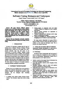
There are four groups of methods, which should be used during development of dependable computing systems: • Fault prevention - how to prevent fault occurrence or introduction. • Fault tolerance - how to provide a service complying to the specifications in the presence of faults. • Fault removal - how to reduce the presence of faults, both regarding the number and seriousness of faults. • Fault forecasting - how to estimate the creation and the consequences of faults. The first two, fault prevention and fault tolerance, may be seen as being dependability procurement, i.e. methodology used to construct a dependable system. The latter two, fault removal and fault forecasting, may be seen as dependability validation, i.e. the methodology used to ensure the dependability of a system. These terms may be grouped according to these classes (see figure 1): • Impairments - undesired, but seldom unexpected, circumstance causing or resulting from un-dependability, i.e. reliance cannot be justifiably placed on the service. These impairments are faults, errors, and failures. • Means - methods and techniques enabling (a) the provision of the ability to deliver a service on which reliance can be placed, and (b) the reaching of confidence in this ability. These means are fault prevention, fault tolerance, fault removal and fault forecasting. • Attributes - these (a) enable the expected properties of a system to be expressed, and (b) allow the quality of the system resulting from the impairments and the means opposing them to be assessed. Faults Impairments

Errors Failures Fault prevention Procurement Fault tolerance

Dependability

Means Fault removal Validation Fault forecasting Availability Reliability Attributes Safety Security

Figure 1: The taxonomy of dependability


5

2.2 Dependability impairments As mentioned above there are three main impairments to dependability: faults, errors and failures. These are all defined by some system property, which is not accepted, i.e., the system deviates in a way from what was intended. In order to be able to distinguish the accepted behaviour of a system from the unaccepted behaviour, a specification of the intended behaviour of the system is needed. When the system behaves in an unacceptable manner, i.e., it does no longer comply with the specifications, a system failure has occurred. The system failed due to some erroneous internal state - an error, i.e., a system state that is different from a valid state in the sense that it is liable to lead to a failure. The conditions, which caused the error, are called a fault. In order to assess the severity of faults and to decide measures for removing them a classification is useful (see Figure 2). The nature of faults distinguishes between accidental faults, faults that appear or are created inadvertently; and intentional faults, faults that are created deliberately. Viewing the origin of faults leads to a number of distinct classes: physical faults, faults related to physical phenomena; human-made faults, which originate from human actions; internal faults, faults internal to a system which, when invoked, produce an error; external faults, faults which result from interference or interaction with the environment; design faults, faults due to imperfections in (a) the creation or modification of a system, or (b) the operating procedures of the system. One can also categorise faults according to their temporal persistence, leading to temporary faults, faults which are present only for a limited amount of time; and permanent faults, faults which are in no way related to point-wise conditions and are always present. Faults

Origin

Nature Phenomenon

Accidental Intentional

Extent

Persistence Phase

Physical Human- External Internal Design Operation made

Permanent Temporary

Figure 2: The classification of faults

This classification of faults allows us to assign distinguishing properties to software faults: software faults are accidental human-made permanent internal design faults, i.e. software can only have faults due to mistakes in design and implementation since it does not suffer from functional changes due to external interactions or ageing. Going from faults to errors, we remember that an error was defined as a system state that is liable to lead to subsequent failure. Whether or not an error leads to a failure depends on a set of factors. A system that incorporates redundancy on some level may mask the error, the activities of the system may cause the error to be overwritten, and the error may produce system behaviour, which in the eyes of the user is not a failure. Again we arrive at the failures. A failure is defined as occurring whenever the external behaviour of a system does not conform to that prescribed by the specification, i.e. the system provides an undesirable service. A system generally does not fail in the same manner. This

6


leads to the definition of failure modes, which are categorised according to domain, perception by the user and consequences. The failure domain1 contains value failures, i.e. the value of the service does not comply with the specifications; and timing failures, i.e. the timing of the delivery of the service does not comply with the specifications. The failure perception, as experienced by the user of the system, can be divided into consistent failures, i.e. failures which are perceived in the same way by all users; and inconsistent failures, i.e. failures for which the users may have different perceptions. The inconsistent failures are normally termed Byzantine faults [Lam82]. The failure consequences can have different levels of severity. A common distinction is benign failures, i.e. failures for which the consequences are of the same order of magnitude as the benefit provided by the service delivered in the absence of failure; and catastrophic failures, i.e. failures for which the consequences vastly exceed the benefit provided by the service delivered in the absence of failure. The creation and manifestation of faults, errors and failures can be described as a chain (Laprie calls it the fundamental chain): …È failure È fault È error È failure È fault È … It is important to notice that not every fault leads to an error, and not every error leads to a failure and so on. A fault is said to be active when it produces an error and dormant otherwise. An error is latent until it is recognised as an error. Errors are detected by error detection algorithms or mechanisms. Failures occur when an error “passes through” the interface of the system. [And83] classifies an error that can be adequately handled by the process in which the error is detected as an internal error. An error that cannot be adequately handled by the process in which it is detected, but whose effects are limited to that process is an external error. A pervasive error is an error that cannot be adequately handled by the process in which it is detected and which results in errors in other processes. Considering the incidence of errors one can make a distinction between persistent errors, i.e. errors which occur more frequently than some predefined threshold, and transient errors, i.e. errors which are not persistent. In practice, classifying an error can only be attempted since it will be impossible to classify all errors correctly [And83]. The deterministic view of failures described above is not always valid. Experiments have shown that software systems fail in rather random ways. In order to describe the nondeterministic manifestation of faults, “bugs”, Gray distinguishes between “Heisenbugs”2, which are intermittent software faults that are not guaranteed to produce an error deterministically as a result of the inputs, and “Bohrbugs”3, which are permanent software faults which, if it caused an error once, will deterministically cause an error every time the program is run with the same input [Gra86].

1

There is another definition of the term failure domain, which is described in section 4. This definition however is completely different from the one described here, so there is no need for confusion. 2 The term “Heisenbug” is derived from the Heisenberg uncertainty principle, i.e. the fundamental limitations on ones ability to measure simultaneously the position and momentum of a particle. 3 The term “Bohrbug” is derived from Bohr’s atom model in which the atom is solid and easily detected with standard techniques.


7

2.3 Dependability means The methods, which can be utilised in order to achieve dependability, are fault prevention, fault tolerance, fault removal, and fault forecasting. Fault prevention and fault tolerance are the procurement for dependability, i.e. ways that provide the system with the ability to deliver a service in compliance with the specifications. Fault prevention is sometimes referred to as fault intolerance [Avi75][Avi76]. Fault removal and fault forecasting are the validation of dependability, i.e. ways to reach confidence in the systems ability to deliver the specified service. Unfortunately, since human activities are involved, these four means are goals that cannot be fully reached. The imperfections in the human activities give rise to dependencies which explain why it is only the combined utilisation of the methods mentioned above which can best lead to a dependable system. The term fault avoidance is often used to describe the close association between fault removal and fault prevention. Fault avoidance is the means of aiming at a fault-free system, e.g. by using the most reliable components, implementing the best techniques for the interconnections of components and carry out comprehensive testing to eliminate hardware and software faults. Fault tolerance, i.e. the ability of an operational system to tolerate the presence of faults [Avi75][Avi76], is carried out mainly by error processing and by fault treatment [And81]. Error processing aims at removing errors from the state of the system, and fault treatment aims at preventing faults from being activated again. In order to be able to undertake error processing, the system must have detected the error and assessed the damage done by it. This gives us four phases, which have to be undertaken in order to tolerate a fault [Ran78][And82][Lee90]: • error detection • damage assessment • error processing (recovery or compensation) • fault treatment (diagnosis and passivation) Figure 3. below illustrates these four phases and how they relate to the process of faults, errors and failures in a system.

Recovery or compensation succeeded

Detection

Assessment initiated

Error overwritten

Error processing

Assessment

Assessment complete

Error detected

Recovery or compensation failed

Fault activated

Fault

Error

Error activated and not detected

Failure System off-line

Treatment Figure 3: The process of faults, errors and failures, and the four phases of fault tolerance

8


Error detection is the detection of an erroneous state, i.e. a state which is liable to lead to subsequent failure. Since an error is a manifestation of a fault the effectiveness of the techniques for error detection are crucial for the success of any fault tolerant system. Damage assessment is carried out when an error has been detected in order to establish more precisely to which extent the system is damaged. This assessment will be highly dependent on decisions made by the systems designer to limit the propagation of errors. When the damage to the system has been assessed, the error may be processed. This may be carried out in two ways: error recovery or error compensation. Error recovery is an attempt to substitute the erroneous system state with one which is error-free. This recovery can be done using either backward recovery or forward recovery. Backward recovery means that the system is brought back to an error-free state recorded in a recovery point - a "snapshot" of the system state - prior to the erroneous state. Forward recovery means the transformation of the erroneous state consists of finding a new state from which the system can operate (often in degraded mode). In error compensation the erroneous state contains enough redundancy to enable the delivery of an error-free service from the erroneous state. When a fault has been successfully tolerated, the system may do fault treatment. The first step in fault treatment is fault diagnosis, which consists of determining the cause(s) of the error(s), with regard to both location and nature. When this is done actions can be carried out in order to prevent the fault(s) from being activated again, i.e. fault passivation. The process of fault treatment is seldom done with the failed system in operation. For instance, a commission of inquiry performs fault diagnosis on the plane that actually crashed in order to gather information about the fault. This information can hopefully be used to passivate the fault that caused the crash - preferably by removing the fault - in other planes (of the same type) which are still in operation. In order to ensure that faults can be tolerated using the four phases4 of tolerating a fault described above, a fault tolerant system is assumed to support some level of redundancy, ensuring that faults can be tolerated using the four phases above. This redundancy consists of additional components and algorithms attached to the system. Avizienis [Avi75][Avi86] divides protective redundancy into the following domains: • Space. Hardware redundancy, which may be divided into static redundancy and dynamic redundancy. The static redundancy is employed to mask the effect of hardware failures within a given hardware module. Therefore static redundancy is also called masking redundancy. When using dynamic redundancy, you actually allow an error to appear in a module. An attempt is made to recover the failed module. The space-domain is denoted H. • Information. Software redundancy, which includes all additional software not needed in a fault-free computer system. This additional software serves to provide for example error detection and recovery. This form of redundancy is often used together with dynamic hardware redundancy. This domain is denoted S. • Repetition. Time redundancy, which incorporates two major strategies: (a) restart of programs after an error has been detected, and (b) repeated execution for error detection. This domain is denoted T.

4

The four phases are error detection, damage assessment, error processing and fault treatment.


9

Redundancy in a domain is denoted with an N, e.g. hardware redundancy is denoted NH. If the redundancy is diversified, this is denoted by a d, as in NdH, which denotes that the redundancy in hardware is comprised of several diverse hardware channels. Using the definitions of these domains and their respective denotations, a description of a non-faulttolerant system (also called a simplex system) is 1H/1S/1T, meaning that the system has 1 hardware channel, 1 program and runs in 1 execution. The fault-tolerance schemes presented in this report will be classified using this notation. Another type of diversity is software diversity, which is frequently used in order to tolerate design faults. Software diversity is logical independence of software components. These diverse software components are functionally equivalent but are implemented in different ways. Diversity may be obtained by different specifications, different algorithms for the same specification, implementations of the same algorithm, and so on. However, experimental data has shown that independence between diverse software components is very hard to achieve [Kni86a]. One important step in building highly dependable computing systems is fault removal, which consists of three steps: verification, diagnosis and fault correction. Verification is the process of checking whether the system adheres to certain properties, so called verification conditions. If it does not, the other two steps have to be undertaken: diagnosing the fault(s) which prevented the verification conditions to be fulfilled, and then performing the necessary corrections. After correction the process of verification is started from the beginning. When a system has been constructed it often desired to make an evaluation of its behaviour with respect to fault occurrence and activation. This evaluation is called fault forecasting and can be carried out in two ways: non-probabilistic, e.g. determining the minimal cutset or pathset of a fault tree, conducting a fault mode and effect analysis (FMEA); and probabilistic, which aims at determining the conformance of the system to dependability objectives expressed in terms of probabilities associated with the attributes of dependability, which may then be defined as measures of dependability. Evaluation of fault tolerant systems often involves the measuring of the coverage of error processing and fault treatment [Arn73], i.e. a measure of the ability of these mechanisms in the system to process the error and treat the fault. This evaluation may be done through testing, using fault injection [Arl89][Gun89].

2.4 Dependability attributes The attributes of dependability allow a systems conformance to dependability objectives to be expressed. These attributes can then serve as measures of dependability and may be more or less emphasised depending on the application intended for the considered computer system. The main dependability attributes are: • Reliability. This can be characterised by a function R(t) which expresses the probability that a system will conform to its specifications throughout a period of duration t. The reliability of a system must be inversely proportional to the rate at which failures occur. The corresponding metric is Mean Time To Failure (MTTF). The definition of this metric is: ∞

MTTF = E ( R(t )) = ∫ R(t )dt 0

10


• Availability. This can be characterised by a function A(t), which expresses the probability that the system will conform to its specification at a given time t. The corresponding metric is Expected Availability (EA). However, for the definition of EA we also need a measurement of Mean Time To Repair (MTTR) which is a measure of service interruption. MTTR is characterised by a function M(t) expressing the probability that a system will be repaired before time t. The definitions of these metrics are: ∞

MTTR = E ( M (t )) =

∫ M (t )dt 0

EA = lim A(t ) = t →∞

MTTF MTTF + MTTR

• Safety. This can be characterised as a function S(t), which expresses the probability that the system will remain safe throughout a period of duration t. The corresponding metric is Mean Time To Catastrophic failure (MTTC) defined as: ∞

MTTC = E ( S (t )) = ∫ S (t )dt 0

• Security. This is the ability of the system to prevent unauthorised access and/or handling of information stored in the system. For most real-time control systems security is not of any concern and will therefore not be addressed in this report.


11

3. Concepts of real-time systems 3.1 Introduction Even though the concept of real-time computing and real-time systems has been utilised for several decades, there has yet to evolve a terminology or a set of basic concepts which is as rigorous as that of the dependability area. At a first glance one might believe that there are as many definitions of what a real-time system is as there are real-time system designers, and this may not be very far from the truth. In [Kri97] Krishna and Shin define a real-time system in the following way: "A real-time system is anything that we, the authors of this book, consider to be a real-time system. This includes embedded systems that control things like aircraft, nuclear reactors, chemical power plants, jet engines, and other objects where Something Very Bad will happen if the computer does not deliver its output in time." Although this definition may be vague, it very much reflects the current philosophy in and approach to the area of real-time systems. However, there are some concepts and terms which are agreed upon in the literature. This section attempts to describe these basic concepts and definitions. The descriptions are based on [Saf75][Melli83][Mello85][Sta88][Kop91][Shi94] [Kri97][Jon97]. Shin states real-time systems as being characterised by three major components and their interplay: time, reliability and environment [Shi94]. Time is the most precious resource to manage in a real-time system. The environment under which a computer system operates is an active component of any real-time system. Reliability is crucial as failure of a real-time system may lead to catastrophic consequences, e.g. economic disaster or even loss of human lives. We will go a little more into detail with these three components.

3.2 Time characteristics Characteristic of a real-time system is that it is a system in which the correctness of the system depends not only on the logical result of the computations, but also on the time at which the result is presented. Of course, no computer systems may use infinite time, however, the time scales of many real-time systems are very fast by human standards. The devices that real-time systems monitor and control often operate on time scales in which a second is an extremely long time. As an example, consider an automobile cruise control system. In order to maintain a smooth ride with only small deviations from the desired speed, the actual speed may have to be monitored 10 times per second, or even more. This may seem rapid in human standards, but it is on the low end of the spectrum in terms of real-time systems. A computer application is normally comprised of a set of co-operating tasks5. These tasks perform some kind of function or provide the system with some kind of service. The tasks of general-purpose computer systems are allowed to execute until they finish, using all the time they need in order to complete. In real-time systems, however, the tasks have certain timeliness requirements, i.e. they have deadlines. The deadlines in a real-time system come from the characteristics of the application and are recursive in nature, i.e. task deadlines will impose deadlines on their sub-tasks, which will then impose deadlines on their deadlines, and so on. 5

A task is sometimes in the literature also called process or transaction.

12


The most common types of tasks are periodic tasks and aperiodic tasks. A periodic task is a task, which is invoked or activated periodically, i.e. once per period T or exactly T units apart. Aperiodic tasks are tasks, which have defined period. A subgroup of aperiodic tasks is the sporadic tasks. These tasks are aperiodic tasks that have a minimum time between arrivals (invocations). A common feature of periodic tasks is that they are time-critical, i.e. the system cannot function properly without completing them in time. An aperiodic task, on the other hand, is a task that is invoked only when a certain event occurs. If the event is timecritical, then the corresponding task will have a deadline by which it must complete its execution and is therefore time-critical. If the event is not time-critical the task will still have to be serviced as soon as possible without jeopardising the deadlines of other tasks. In some systems it is of importance not only that the result is in time, i.e. presented prior to a deadline, but also that it is on time. This means some results may be useless if they are produced before a certain time (maybe one could refer to the earliest point in time when a value is needed as a birthline as opposed to a deadline). There may be a window in time when the result of a task is valid and required. Also, some computations are depending on results from other computations. These requirements manifest themselves as precedence requirements, i.e. a task may require the results from one or more tasks before it can start its own execution. When considering periodic events one always has to take into account that there may be a certain jitter in the period. The jitter is the amount of uncertainty in the period, i.e. the time between two events is the period T plus or minus a certain time ∆t. The jitter is usually an undesired property of periodic events and may disrupt the timing of computations. Therefore it is important to eliminate, or at least bound, this uncertainty in the period of tasks. The deadlines of real-time systems can be classified as hard, firm, and soft. A deadline is said to be hard if the consequences of not meeting it can be catastrophic. In [Sta88] systems with deadlines of this kind are called hard real-time systems. Periodic tasks usually have deadlines of this kind. A deadline is said to be firm if the results produced cease to be useful as soon as the deadline expires, but consequences of not meeting the deadline are not very severe. The deadlines of many aperiodic tasks belong to this category. A deadline, which is neither hard nor firm, is said to be soft. The usefulness of the results produced by the corresponding task decreases over time after the deadline has expired. The term soft real-time system usually refers to real-time systems that are not hard, i.e. failing to meet a deadline does not have catastrophic consequences. Real-time systems also often require concurrent processing of multiple input. A concurrency requirement can be set up for most systems, real-time systems as well as non-real-time systems. However, true requirements for concurrency usually involve correlated processing of two or more inputs over the same time interval and are quite different in character from the overlapping of transactions in a multi-user interactive business system. A real-time system must also be predictable, i.e. the tasks must have guarantees that their constraints will be fulfilled. In a simple system, predictability means that it is possible to show, at design time, that all timing constraints in the application will be met with 100% certainty. In more complex system, the meaning of predictability varies from one task to another. Some critical tasks may still require a 100% guarantee that their constraints will be satisfied. Such tasks are usually periodic tasks with hard deadlines. It is important to note that in order to be able to deliver 100% guarantees to a task, the complete characteristics of the tasks, with regard to its execution time and arrival time, would have to be known a priori. It is unlikely that one would have all this information at design time.


13

Tasks, which do not need 100% certainty that their constraints will be fulfilled, may be satisfied with either probabilistic or run-time deterministic guarantees. Probabilistic guarantees are either (a) a certain percentage of tasks are guaranteed to meet their constraints, or (b) a given task has a certain probability of meeting its constraints. Note that in some cases these two notions are equivalent. Run-time deterministic guarantees mean that when a task is invoked or activated the system determines whether or not the constraints of that task can be satisfied without jeopardising the guarantees given to other tasks. If the constraints can be satisfied, the task is accepted and provided with a 100% guarantee that it will meet its constraints. If the constraints cannot be satisfied the task is rejected. This has the consequences that, at design time, one cannot know which task will meet its constraints.

3.3 Environment characteristics Most real-time systems typically consist of a controlling system and a controlled system, i.e. a computer in conjunction with some external process (or processes). The controlled system the external process - is said to be the environment of the controlling system (see Figure 4.). The objective of the controlling system is to obtain information on the operation of the external process, i.e. measure important variables, and to manipulate it in some desired manner, i.e. control the way in which it operates based on the information previously acquired. Figure 3 below visualises a real-time system in its environment.

Real-time system A A

Environment

A S

Real-time software

S S S

Figure 4: A real-time system and its environment.

S

denotes sensors, A

denotes actuators.

In order to measure the surrounding environment, real-time systems often make use of devices which act as the senses of the system, i.e. sensors. In a broad sense any system that accepts input may be said to be sensing what is occurring in its environment. For real-time systems these devices are typically sensors such as thermocouples, optical scanners, etc., enabling the system to collect a continuous stream of input data. This is analogous to the functioning of the senses in a living creatures, i.e. eyes, ears, touch, and so on. In order to manipulate its environment, a real-time system often contains devices which effect physical changes as sensory inputs occur, so called actuators. Actually, in some sense any system, which produces output, effects its environment. However, characteristic of real-time systems is that the outputs produced often are continuous in nature. Thus the operation of a real-time system often mimics human patterns such as eye-hand co-ordination. A system of this kind also effects its environment in a way which often is quite easy to sense, e.g. by changing temperatures, valve positions and so on, rather than in the more abstract way of

14


merely producing information which is acted upon by an operator. Bearing this in mind, it is easy to understand that the reliability of the output of a real-time system is often crucial. Catastrophic consequences may be the result should the output be faulty in some way, either by having a faulty value or by being late.

3.4 Reliability characteristics The close relation between the real-time system and its environment puts requirements on the system that it performs its required actions during its entire operational time, i.e. it has to be reliable. Reliability for real-time systems is defined as the probability that the system will not fail during. The reliability-concept in the area of real-time systems is very much the same as that of the dependability-area. The concept of safety is not used as a stand-alone concept but is often treated as equivalent to reliability. Since this section is a summary of the concepts and terminology used for real-time systems, the terms reliability and safety are considered equivalent in the remainder of this section. However, it is desirable to distinguish between the two, and the following chapters and sections will use this distinction.. Since real-time systems are more and more employed to control critical functions of complex constructions, such as aircraft, nuclear power plants or automobiles, these requirements become more and more important. The reliability of a real-time system depends not only on the correctness of its results considered from a value-domain point of view but also on the correctness in the time-domain, i.e. a value may be useless if it is to late (as discussed above). A reliable real-time system can be said to be one , which in the event of failures in the system, still has an effect on its environment that does not jeopardise safety, i.e. they must be fail-safe. A common distinction is made between fail-silent systems and fail-operational systems. A fail-silent system is one, which in the event of system failure leaves the controlled system in a safe state and then stops interacting with its environment. In a fail-operational system the interactions with the environment are limited to inherently safe operations, i.e. the functionality is degraded. Consider for example a throttle-by-wire system in an automobile. The throttle is controlled by an electronic control unit using the pedal as a sensor and the air intake of the engine as an actuator and is not manoeuvred through a physical link between the pedal and the air intake as in normal throttle systems. If the control system is fail-silent it may stop the airflow to the engine, which then is muzzled. If the control system is failoperational it may set the airflow to a minimum for which the engine generates enough torque in order for the driver to get home (the throttle system is then often referred to as being in a limp-home state). Another common application for fail-operational systems is that of aircraft control systems - should they fail in mid-air the pilot must still be able to land the aircraft. The combined requirements of the performance (timeliness) and the reliability of a real-time system is often referred to as the performability of a real-time system. This term very much summarises the common requirements on a real-time system: the output must be correct the first time and on time. Sometimes, requirements on the availability of the system may also incorporated in the term performability, e.g. in telecommunication systems. A common way of measuring a system’s performability is to define a set of accomplishment levels for the process the system is set to control. These accomplishment levels are different levels of performance as seen by the user and are associated with certain behaviour of the system. The performability of a system is then given as a vector containing the probabilities of achieving each of these accomplishment levels.


15

4. Software fault-tolerance techniques 4.1 Introduction The key to fault-tolerance in general is redundancy. As described in section 2.3.1 there are three domains in which it is possible to achieve redundancy: Space (the H-domain) - e.g. a system which has several hardware channels each executing the same task; Information (the S-domain) - e.g. a system which incorporates enough redundancy into its data structures in order to be able to recover the contents in the event of error detection; or Repetition (the Tdomain) - e.g. a system which in case of a detected erroneous state restarts the execution of the faulty module. Two major software fault-tolerance schemes have evolved through the years: the recovery block (RB) scheme and the N-version programming (NVP) scheme. Using Avizienis’s redundancy notation described in section 2.3 we classify the systems which implement the RB scheme as 1H/NdS/NT-system, i.e. there is only one hardware channel (1H), and the faults are tolerated by executing several diverse software modules (NdS) sequentially (NT). Systems implementing the NVP-scheme, on the other hand, are NH/NdS/1T-system, i.e. the system has a number of (identical) hardware channels (NH) each executing one of the diverse software versions (NdS), hence no redundancy in time (1T). Some systems may be NdH/NdS/1T, meaning that they are NVP-systems in which also the hardware channels are diverse. One thing common to most of the current software fault tolerance techniques is that they make use of diverse software modules performing the same logical operations. This is done in the belief that independently developed implementations of a software module would also fail independently, i.e. they would not fail for the same type of input. The idea of multiple computations actually was suggested already back in 1834, when Dr. Dionysos Lardner wrote the following with regard to Babbage’s calculating engine: “The most certain and effectual check upon errors which arise in the process of computation, is to cause the same computations to be made by separate and independent computers6; and this check is rendered still more decisive if they make their computations by different methods.” The assumption of independence between independently generated software versions has however been questioned by experimental data [Kni86a]. The main argument for using multiple versions of a software module is, as stated above, that they should fail independently. They are said to have different failure domains7 in the input data space (see Figure 5. below). Therefore using several diverse version may increase the probability that some of them execute without entering a failure domain.

6

In 1834, the term computers referred to people performing computations. Note that this definition of failure domain differs from that defined in section 2 on concepts of dependability earlier in this report.

7

16


Program path

Failure domain

Input space

Figure 5: A program’s failure domain in the input space.

Besides the recovery block scheme and the N-version programming scheme there are a number of fault-tolerant schemes which are based on either one of these schemes or a combination of both. There are also other schemes, such as data diversity. The following sections describe several of these software fault-tolerance techniques.


17

4.2 Recovery Block (RB) 4.2.1 Basic description The recovery block (RB) concept was introduced by Horning, Randell and others in [Hor74][Ran75]. Using the notation on redundancy presented above, the recovery block scheme is classified as 1H/NdS/NT. This means that the system has one hardware channel, i.e. no redundancy in the hardware; has redundant in software - it uses multiple diverse modules performing the same task; and is also redundant in time, since the multiple modules are executed sequentially in the event of errors. Horning describes a Recovery block as being a "firewall in time". The basic elements of a recovery block are the following: • one primary module - a program module which performs the desired operation. This is an ordinary program block or; • zero or more alternate modules - modules which should be such that they perform the same desired operation as does the primary module, however in a different way; and • one acceptance test - a test which is executed on exit from the primary and alternate modules to confirm that the results produced are acceptable to the environment of the recovery block. In order for the recovery block to be able to provide any degree of fault tolerance and continued service in the event of module failure, there must be at least one alternate module. All alternate modules should deliberately be different from the primary module, and also from each other, i.e. software diversity is employed. If all the modules would be the same, or even just similar, not much would be gained since they would all fail in the same way when working on the same input data. The modules of the recovery block may themselves incorporate inner recovery blocks, i.e. the recovery block scheme can be nested. The acceptance test yields a binary decision as to whether or not the results produced by a module are acceptable. In addition, the recovery block scheme requires a recovery cache, i.e. a structure which provides functionality for storing essential information of the current system state in so called recovery points or checkpoints - snapshots of the system state. Figure 6. below shows the basic structure and flow of a recovery block. Recovery block Input

Capture checkpoint and store in recovery cache

Acceptance test

Primary

S w i t c h

Passed

Output

False

Failure

Failed

Alternate 1

. . . Alternate N-1

Restore checkpoint from recovery cache

True

Candidates not exhausted and deadline not exceeded

Figure 6: The basic structure and flow of a recovery block.

Upon entry into a recovery block a checkpoint is established. This checkpoint is stored in the recovery cache, and contains all relevant data describing the current state of the system as seen from the recovery block, i.e. only the parts of the system data which are relevant for the recovery block need to be stored. When the checkpoint has been stored the primary module is


18

executed. After its execution the produced results are submitted to the acceptance test. If the results are considered OK by the test, the recovery block is terminated and the results are passed as the output of the recovery block. The other possibility is that the test fails. The acceptance test can reject the results of a module on account of these four causes: 1. an error in the operation of a module, explicitly detected by the acceptance test; 2. the module fails to terminate, detected by a time-out; 3. en error is detected during execution of a module by one of the implicit error detection mechanisms (e.g. division by zero); or 4. an inner recovery block has failed due to all modules being rejected either explicitly or implicitly and therefore recovery on this level is no longer possible. Should the results not be accepted, a recovery procedure is started. This procedure will restore the system state to that which is described by the checkpoint established at block entry and is stored in the recovery cache. This form of recovery is called backward recovery or rollback recovery in that it provides all modules, primary and alternates, with exactly the same experience of the system state when their respective executions start, i.e. the time can be said to be turned back. When the recovery is complete the first alternate module is executed, and on exit the results are again submitted to the acceptance test. If the test is successful the recovery block terminates, otherwise the system state is again recovered in the same manner as before and the second alternate module is executed. Once again the results will be checked by the acceptance test. This chain of events will continue until (a) a module produces results which pass the acceptance test, thereby terminating the recovery block and returning the results as output of the recovery block, or (b) all modules have failed and an error is raised to the environment. From a programming language point of view recovery blocks could be supported syntactically. A recovery block could look something like the code example with a primary module and one alternate module in Figure 7. below. An attempt to provide Ada95 with Recovery Block primitives is made in [Ker96]. ... ENSURE Atest_1( output_candidate ) BY output_candidate := calculate_pressure(); ELSE_BY output_candidate := simulate_pressure(); ELSE_ERROR output_candidate := fail(); END ...

Figure 7: Code example of a recovery block

A special case of the recovery block structure has only a primary module and no alternate modules. Such a structure would not have any need for checkpoints or a recovery cache since the state of the system is not required to be reverted back to the state the system had at block entry. Should the primary module fail, an error will be raised to the environment immediately.


19

4.2.2 Problems and considerations The original recovery block scheme may at first seem very simple in structure. However, there are some considerations to have in mind. The considerations are related to the following issues [Ran75][Ran78][Lee78]: • • • • • •

the types of faults tolerated by recovery blocks designing the primary and alternate modules designing the acceptance test designing the recovery cache mechanism system overhead of the scheme the domino-effect

These considerations and problems are discussed below. Faults tolerated by recovery blocks The original aim when introducing the recovery block scheme was concentrated at aiding the design of error detection and recovery facilities for coping with software design faults, although Horning et. al realised that the scheme could also handle many types of hardware faults. The types of faults that are tolerated are classified as algorithmic faults [Lee78]. For hardware algorithmic faults are missing or incorrect connections between components. In software all faults are algorithmic faults. Algorithmic faults are residual design faults rather than component faults. Recovery blocks are designed to tolerate these algorithmic faults, both for software and hardware, although the scheme is used mostly against software faults. The scheme employs backward error recovery, hence there is no need to make assumptions about the faults that can occur and the damage they may cause. Designing primary and alternate modules A key characteristic of the recovery block is that all modules, primary as well as alternates, start there execution from the same system state. This has the effect that the different modules can be design independently of each other - the designers of one module need not have knowledge about the design of other modules. Equally, the designer of a program containing a recovery block is not concerned with which of the modules is actually used to provide the results of the recovery block. This is used as an argument that an increase in the size of a program not necessarily increases the complexity of it. Again, we come across the concept of software diversity. It has been shown experimentally that independent implementations of one single system specification are in fact not diverse, i.e. they would not fail independently [Kni86a]. This study shows that even though the teams of programmers are independent of each other, with different levels of expertise, backgrounds, and education, the defects made during development, which later appear as residual faults in the programs, are not independent. It has been argued that, if the primary module provides the full intended service of the system and the alternate modules provide increasingly degraded service, i.e. the lower the level of the alternate the more degraded the service, would make the development of the alternate modules less error prone. Since the modules providing the degraded service would be simpler to design, the hope of designing without faults consequently gets greater. Designing the acceptance test The acceptance test of a recovery block can be regarded as an assertion of the effects of the execution of a recovery block, which are required for the correct operation of the surrounding program. The test provides a binary decision as to whether the results have been accepted as satisfying this assertion, thereby stating whether the results are acceptable by the surrounding


20

program. For every recovery block there is one single acceptance test invoked for the outputs of all modules in that recovery block. Acceptance tests usually fall into one of the following categories: (a) satisfaction of requirements, (b) accounting tests, (c) reasonableness tests, and (d) computer run-time checks. The distinction between these may sometimes be blurred. Ideally, an acceptance test can give absolute certainty that the asserted results are either correct or incorrect. However, this may not be feasible for some reasons [Lee78]: (a) the performance of the test may become to low, (b) the alternate modules may provide a degraded functionality as compared to the primary module, (c) the complexity of the design of an acceptance test make it prone to design faults. The major problem of those given above would be that the acceptance test is subject to software design faults, since the test itself also is written in software. The more complex the operations performed in a module the more complex will the acceptance test need to be. In order to detect as many errors as possible in the results produced by a module, the acceptance test would have to know the complete characteristics of the operations performed by it. This in turn makes the acceptance test highly error prone. Analysis has shown that the acceptance test is the most crucial component of the scheme if reliability is to be increased over that of the primary module [Sco83]. An imperfect acceptance test may even decrease the reliability of the entire system compared to that of a highly reliable primary module since it may classify correct results as incorrect rendering them useless. If the alternate modules of the recovery block only provide degraded service compared to the primary module, the acceptance test has to be designed with knowledge about this. This means that the acceptance test can only be as rigorous as a check on the results from the module, which produces the most degraded service (the weakest module). Using for example nested recovery blocks as described in Figure 8. can circumvent this problem. ... ENSURE TRUE BY ENSURE best_acceptance_test() BY best_module(); ELSE_ERROR fail(); END ELSE_BY ENSURE next_best_acceptance_test() BY next_best_module(); ELSE_ERROR fail(); END ... ELSE_ERROR fail(); END ... Figure 8: Nested recovery block for degraded functionality using multiple acceptance tests

Designing the recovery cache mechanism It is assumed that in order to be able to restore the system between invocation of the modules only a few global values need to be stored, since most of the operations in the modules are conducted using local variables. This makes the design of a recovery cache mechanism very straightforward and easy. However it is likely that there may be some objects which cannot


21

or should not be placed in the recovery cache. In order to be able to restore the state of the system in the event of recovery, it is imperative that the modules do not gain direct access to the surrounding system in order to manipulate it, e.g. via actuators in a control system. Once the actuator has effectuated the change, it may be irreversible. This problem may be solved using multi-level systems, i.e. the system is constructed with multiple levels of abstraction, and in that way provides recoverable objects built on unrecoverable objects. The recovery cache is considered to be a "hard core" component of the recovery block scheme, i.e. it is assumed that the recovery cache is reliable and never fails [Lee78]. It is argued that the design of a recovery cache is sufficiently simple so that it can be ensured that no residual faults are present. System overhead of the scheme Since the recovery block scheme uses a recovery cache and backward error recovery, it introduces physical and temporal overhead, i.e. compared to a "clean" system a system implementing recovery blocks uses more space (memory) and more time. The overhead in space is mainly due to the extra space needed to store the code of alternate modules and the acceptance test, and the space needed for the recovery cache. The overhead in execution time is mainly dependent on the time required to evaluate (execute) the acceptance test and on the implementation of the recovery cache. In [Hec76] Hecht considers the use of recovery blocks in real-time systems. He concludes that the scheme is suitable with the addition of watchdog-timers in order to check that results are available in time. The Domino Effect The original recovery block scheme only considers single process programs with sequential structure. In many of the current computer controlled applications (especially embedded control systems), the program is divided into several concurrent tasks8 communicating with each other. Consider a system with three processes using recovery blocks and interacting with each other as shown in Figure 9. below. Every vertical bar depicts an active recovery point, i.e. each task has entered four recovery blocks that it has not yet left. Every dotted line depicts interaction between tasks. 1

2

3

4

Task 1 1

2

4

3

Task 2 1

2

3

4

Task 3 time Figure 9: The Domino Effect

Should task 1 fail, it will be backed up to its latest recovery point, i.e. recovery point 4. The other two tasks would not be affected. If task 2 fails it will be rolled back to its fourth recovery point. Since it has interacted with task 1 after the recovery point was established, task 1 is required to roll back to the recovery point prior to the interaction, i.e. recovery point 3. Should task 3 fail, all the tasks would have to be rolled back to the first recovery points! This kind of uncontrolled rollback is called the domino effect [Ran78]. This effect can occur 8

As described in section 3 on real-time system concepts earlier in this report.


22

when these two circumstances coincide: 1) the recovery block structures of the various tasks are uncoordinated, and take no account of interdependencies caused by their interactions; 2) each member of any pair of tasks can cause the other to be rolled back.

4.2.3 Extensions In the original recovery block scheme, only single task programs with sequential structure are considered. Using the scheme without alterations in applications with concurrent tasks, which interact with each other, may in backward error recovery eventually lead to the domino effect, as described above. This effect can be avoided if either one of the two causing circumstances mentioned above is removed. Randell presents a technique that structures the interactions conversations [Ran78]. A conversation is in effect a recovery structure that is common to a set of two or more tasks. The tasks within a conversation are only allowed to interact with each other, no interactions can be allowed outside the set. The conversation structure is illustrated in Figure 10. below. Every vertical bar depicts an active recovery point, i.e. each task has entered four recovery blocks that it has not yet left. Every dotted line depicts interaction between tasks.

Task 1

Task 2

Task 3 time Figure 10: Parallel tasks with conversations

The tasks, which participate in a conversation, need not enter the conversation structure at the same time, but once they enter they must give up the right to interact with tasks outside the conversation. There is no limit on the interaction between the tasks inside a conversation, though. At the end of the conversation all participating tasks must satisfy their respective acceptance tasks and none may proceed until all have done so. Conversations can of course occur within other conversations, but then only between tasks which already participate in the surrounding conversation as illustrated in Figure 11a. Structures as that shown in Figure 11b. must be prohibited. Task 1

Task 1

Task 2

Task 2

Task 3

Task 3 time (a)

Figure 11: a) Nested conversations, b) invalid conversations

time (b)


23

4.3 N-Version Programming (NVP) 4.3.1 Basic description The concept of using multiple computations in order to detect and correct failures made during these computations has been known since Babbage built his calculating engines. In modern times, the usage of multiple versions of a software module in order to tolerate faults has been in use since the 1960’s, but an effort to investigate the properties and constraints of this approach was not undertaken until Avizienis introduced a generalisation of the multiple computation method called N-version programming (NVP) in 1977 [Avi77]. He defined Nversion programming as the independent generation of N ≥ 2 functionally equivalent programs from the same initial specification. These N versions would run on several hardware channels producing results which are subject to some decision mechanism, usually a voter. If a majority of the N versions agree on the result, this result will be used as the output. If no majority agreement can be obtained, the system fails. Figure 12. below shows the basic structure of the N-version programming scheme. In a sense, the NVP approach can be said to be the software equivalent of the N-modular redundancy for hardware where several hardware channels are used to mask hardware failures. Using Avizienis’ notation on protective redundancy, we can denote a system implementing the N-version programming scheme as an NH/NdS/1T-system or an NdH/NdS/1T-system depending on whether the hardware channels are identical or different from each other.

N-version programming Version 1

Input

Version 2

. . .

S y n c h

Voter

Majority agreement

Output

No agreement

Version N

Failure

Figure 12: Basic structure of the NVP-scheme.

The basic elements of the N-version programming approach are: • the initial specification - this is the specification of the functionality which is desired by the software; • N software versions - software modules which all are independently generated from the initial specification; and • a decision mechanism - a mechanism which decides what the final result of the computations will be using the results from the N versions as input. • a supervisory program - this is a software structure used to drive the N versions and the decision mechanism. The most crucial part of the N-version programming approach is the initial specification. This specification is considered the “hard core” of the approach and is required to be unambiguous yet trying to impose as little as possible in design methods or algorithms to be used on the implementers. The N software versions are generated independently from the initial specification. Independently here means that they are developed by different teams of engineers, using different algorithms and maybe even different languages, compilers, operating systems. The teams themselves should also be diverse, i.e. they should have different backgrounds, both

24


educational and ethnical. The N versions will be functionally equivalent and have identical interfaces to the surrounding software. The decision mechanism uses all results from the N versions to make a decision on what the final result shall be. This decision mechanism is often a voter opting for a majority agreement between the N versions. The comparison may be for total equality, i.e. the results must be bitwise identical (“exact voting”). However, this may in many applications not be applicable, since the output of the N versions may be numerical values and thus continuous in nature. These values may differ due to the hardware’s limited ability to represent for instance real numbers (they are usually truncated). This yields a need for the definition of an allowable range of discrepancy, i.e. the comparison cannot be made for bit-wise equality (“inexact voting”). Any version which generates results that differ from the acceptable results is designated as a disagreeing version. The actions taken when a version disagrees may be that they are taken out of future computations or they may be subject to recovery attempts. The cs-indicators may guide the decision algorithm in its choice of action. In order for the decision mechanism to do its job, the outputs of the N versions must be synchronised. The supervisory program supervises all interaction between the N software versions and the decision mechanism. It also handles the part of the synchronisation mechanism which puts the versions in different states of operation. Originally a version is in an inactive state. When it is invoked by the supervisory program it enters a waiting state. The version waits until it receives a signal representing a request for service, i.e. computation. This signal transfers the version into a running state. If any terminating condition is signalled, the execution will be aborted and the version will go back to the inactive state. Otherwise, it generates a result when a synchronisation point is reached, notifies the supervisory program that a result is ready, and returns to the waiting state. These states and the transition between them are illustrated in Figure 13. below. Invoked Inactive

Waiting Cross-check point condition satisfied Service required

Terminating condition satisfied Running

Figure 13: The state transition of a version

4.3.2 Problems and considerations The NVP approach incorporate some issues which may cause problems or just have to be considered: • • • • •

the types of faults tolerated by N-version programming the initial specification generating independent versions the decision mechanism system overhead of the scheme

These considerations are discussed below


25

Faults tolerated by N-version programming The purpose of N-version programming is to provide either fault-tolerance or fault-detection with respect to software (design and implementation) faults [Avi77]. The scheme aims at tolerating or detecting these faults by trying to minimise the probability of similar errors at decision points in N-fold computations [Avi85]. This shall be achieved by independent generation of multiple functionally equivalent versions from the same initial specification. A fundamental conjecture is that the independence of programming efforts will greatly reduce the probability of identical software faults. The scheme may also be able to tolerate faults in the hardware, since it utilises several hardware channels. The errors produced by faults in components may sometimes not be distinguishable from those created by software faults. Hence, many hardware faults can be treated as though they were software faults with regard to their effect on software execution. Of course, recovery has to be quite different for hardware faults compared to software faults. Initial specification Design faults are caused by errors made during the translation of the original system specifications into operational forms [Avi75]. This is the main reason that the initial specification has to be unambiguous and complete, so that design faults due to imprecise requirements are avoided. Also, as stated earlier in this report, a failure is defined as the initial deviation of the system from the specification, or desired service. Ideally, there is no room for interpretation of the requirements in the specification. Yet, in order for the development teams to independently create software modules which are as diverse as possible from each other, the specification must impose as little as possible in design methods, algorithm choices, and so on. In order to try to make the programming effort less dependent on the specification, experiments were conducted using several versions of the initial specification as well [Kel83]. These versions were diverse, i.e. they were written in three different languages. One was written in the formal specification language OBJ, one was written in PDL (Program Design Language), and one was written in plain English. The result of this study shows that the diversity in the specification did not have a profound impact on the residual faults in the produced software versions. Generating independent versions From the initial specification, several software versions shall be generated independently. As stated above, most design faults are caused by errors in when the requirements in the specification are implemented by software engineers. Therefore, it is believed that if independent programming teams, with different background, education, levels of experience, etc., are employed to produce the various versions, these will be diverse. This diversity is said to minimise the probability of residual software design faults leading to erroneous decisions caused by similar or coincident errors occurring in two or more versions. This assumption is the fundamental conjecture of the N-version programming approach. According to Avizienis the effectiveness of the NVP approach depends on the validity of the fundamental conjecture [Avi85]. The assumption of independence has been experimentally evaluated in [Kni86a]. In this experiment no less than 27 different versions of a program were evaluated. The result of study shows that the versions cannot be considered to fail independently. Although this may seem to invalidate the entire NVP approach, empirical studies in [Kni86b] on 3-version systems have shown that even if the assumption of independence does not hold, the probability of failure of a system can be decreased using the NVP approach. However, this decrease was not nearly as high as that derived through simple models of the NVP approach.

26


Decision mechanism According to Avizienis in [Avi85] the main difference between the decision mechanism of the NVP approach - the voter - and the acceptance test of the recovery block approach is that the voter need not know the characteristics of the application, i.e. the results of the computations. Hence, it may be possible to construct a general decision mechanism which can be used for several different applications. This is certainly true for comparisons which demand equality in the result bit by bit. However, as soon as the results are numerical and continuos in nature (i.e. real-number values), bit-wise equality may not be applicable. In these cases inexact voting, i.e. allowing some discrepancies between the results, has to used. The range that is assumed to be correct may be defined by a distance function over the space of the possible results. Another kind of inexact voting is one that ignores cosmetic differences between strings of characters. An implementation of inexact voting in the form of a distance function may be very application specific., hence the difference between the NVP approach and the recovery block approach as stated above is decreased. The problems that apply to the acceptance test of the Recover Block approach may also apply to the voter of the NVP approach. The problem of inexact voting is even further accentuated by the fact that the N versions may produce multiple correct results, i.e. for a given problem there may exist several correct solutions. System overhead of the scheme A system implemented with the NVP approach makes use of several hardware channels to execute the N versions, hence the temporal overhead will mainly consist of the extra time it takes to execute software for synchronisation of the N versions and the decision algorithm. Such a system has of course considerable redundancy in space, mainly due to the multiple hardware channels, but also due to the space needed to store the N versions.

4.3.3 Extensions In the original NVP approach disagreeing versions, i.e. versions that have produced a result which is considered erroneous, are simply removed from future computations. Hence, the original system will fail when the accumulation of failures is large enough to saturate the fault-masking ability, i.e. when N-2 versions have failed (N-1 if the decision mechanism can detect errors in each individual version). In order to extend the up time of an NVP system, recovery of failed versions is suggested. In [Tso86] and [Tso87], Tso et al. propose forward error recovery in the form of Community Error Recovery (CER) for failed versions. This way of recovery makes use of the assumption that at any given time during execution there exists a majority of good versions which can supply information to recover the failed versions.


27

4.4 Consensus Recovery Block (CRB) 4.4.1 Basic description The consensus recovery block was introduced by R.K. Scott et. al in 1983 [Sco83]. This scheme is actually a synthesis of the original recovery block and N-version programming (see Figure 14. below). When the consensus recovery block is invoked it begins the computation as a normal NVP-structure, i.e. the N versions are executed in parallel and the results are voted upon. A basic assumption is that no similar errors, i.e. erroneous results resembling each other, will occur. This means that if two or more versions can agree upon a result, their output is considered to be correct. If no agreement can be achieved, the results from the N versions will be examined by an acceptance test, starting with the results of the best version and continuing with the next best version and so on. The first result that passes the acceptance test will be used as the correct output of the computation. This implies that even though no agreement could be achieved among the N versions, the results they produced are not necessarily erroneous. If no result passes the acceptance test, a failure is raised and the handling of it, e.g. recovery, is moved to the next higher level of the system.

Version 1

Input

Output

Agreement

Version 2 Voter

. . .

No agreement

Version N

. . .

Accept

Output

False

Failure

AT

True


Figure 14: The basic structure of a consensus recovery block

With Avizienis’ redundancy classification we can describe this system as an NH/NdS/1Tsystem or an NdH/NdS/1T-system, i.e. the N diverse software versions execute concurrently on separate hardware channels (which may or may not be diverse). The fact that the N versions are executed in a parallel fashion upon entering the consensus recovery block eliminates the requirement of a recovery cache, since the versions do not need to be rolled back in the event of failures. This scheme also reduces the problem of the possibility of multiple correct results from the N versions. And, since the results of the N computations are voted upon to determine the need to execute the acceptance test, the crucial part that the acceptance test plays in the recovery block is reduced. Reliability modelling performed in [Sco87] shows that the consensus recovery block is more reliable than both the original recovery block and N-version programming.

4.4.2 Problems and considerations The consensus recovery block does have some drawbacks, though. One of the major disadvantages is the cost of implementation, since there are a lot of modules that have to be


28

developed: N independent versions, a voting mechanism and an acceptance test. Besides the cost aspect, this means that all the problems that apply to the development of N independent versions and the voting mechanism presented for the NVP scheme also apply to some extent to the consensus recovery block. Also the problems applying to the development of the acceptance test described for the recovery block are valid for this scheme, even if the critical role of the acceptance test is reduced. The numerous parts of the consensus recovery block also introduce a system overhead which may not be acceptable in many real-time control systems. The basic assumption of the consensus recovery block, i.e. that there will be no similar errors in the results of the N versions, may be problematic, since similar errors cannot be ruled out. Should there be similar errors and these results are chosen by the voting mechanism as the basis of the agreement, the output of the consensus recovery block will be erroneous.

4.5 Distributed Recovery Block (DRB) 4.5.1 Basic description The distributed recovery block (DRB) was introduced in 1984 by Kim in [Kim84]. The aim was to integrate software and hardware fault tolerance into one single structure since it may be very difficult to distinguish between software faults and hardware faults. The DRB is as the name suggests based on the recovery block scheme. The main difference between the both schemes is that both the primary and the alternate modules are replicated and are resident on two or more separate nodes interconnected by a network. Software faults are hopefully coped with in the traditional recovery block fashion, and hardware faults are handled by the distribution of computation among several nodes. Accept Version A

AT

Version B

True Input

Primary node


False

Output

Version B

AT

Version A

True Backup node


Accept

False

Failure

Figure 15: The basic structure of a distributed recovery block.

Figure 15. above illustrates a distributed recovery block with two nodes, one primary node and one backup node, and two software modules, so called try blocks. Each of the two nodes has the two try blocks resident as well as the acceptance test. Both nodes use the same input data for the computations. The primary node will execute the primary try block and the backup node will execute the alternate try block, and this execution is concurrent. If both nodes pass the acceptance test the primary node notifies the backup node and the results of the primary node will be used as output. Should the primary try block fail to pass the acceptance test, the primary node notifies the backup node of the failure. If the alternate try block on the backup node has passed the acceptance test these results will be used as output and the backup node will assume the role of the primary node. If, on the other hand, the


29

backup node fails first, this will not affect the primary node. In case a node fails, the node will make a roll back and retry with its other try block. A DRB-system is classified, using Avizienis’ redundancy classification, as an NH/NS/1Tsystem or an NdH/NdS/1T-system, since the software versions execute concurrently on several hardware channels. The system in Figure 15. above is an 2H/2dS/1T-system. Since the try blocks are executed concurrently, a results will generally be immediately available for output from the distributed recovery block, hence 1T. This means that the recovery time for failures is much shorter than if both try blocks were to execute on the same node. If the primary node stops execution altogether, the backup node will detect this by the absence of an update message from the primary node within a predefined time limit. This check on the time is actually part of the acceptance test. In [Kim89] the distributed recovery block was implemented in a radar tracking application. Results from this experiment showed an increase in the average response time from 1.8 ms to 2.6 ms, an average of 8% processor utilisation for the acceptance test, and that backup processing was not a significant portion of total workload. These results were considered acceptable.

4.5.2 Problems and considerations As described above, when the primary node fails it will make a rollback recovery and try to take the role of the backup node. However, in order to complete the transition to the backup status, the node must succeed in its recovery, i.e. it must execute the alternate try block, in order to keep the state data consistent with the companion node. This implies that the data arrival rate and system computing capacity must be such that it is possible to perform a rollback recovery without violating timing requirements. The DRB scheme was originally developed for command and control applications in which data is collected by interface processors and distributed over a network, and in which output data from one pair of processors was input data for another pair of processors. During attempts to apply the DRB constructs to real-time control systems, a few changes had to be made. These changes made the structure so different from the original DRB scheme that it was called the extended distributed recovery block, which is described in section 4.6 below.

4.6 Extended Distributed Recovery Block (EDRB) 4.6.1 Basic description The extended distributed recovery block (EDRB) was introduced by Hecht et al. in 1991 [Hec91a] [Hec91b]. This scheme is based on the distributed recovery block scheme described in section 4.5 above. An EDRB has a top-level structure like the one illustrated in Figure 16. below. Supervisor

Operational nodes Node pair

Node pair

Figure 16: The top level structure of an extended distributed recovery block with two node pairs.


30

As can be seen, there are several kinds of nodes in an EDRB structure. Nodes responsible for control of the process and related systems are called operational nodes. These nodes are often critical since they provide some kind of real-time service and store non-recoverable state information. Therefore they are redundant. The operational nodes are clustered in sets of two, so called node pairs. The members of a node pair exchange periodic status messages called heartbeats. A node in a node pair can recover from failure in its companion node if the malfunction is declared as a part of the heartbeat message. Should one of the nodes in a pair stop sending its heartbeats, the other node will request a confirmation of the first nodes failure from a second kind of node called the supervisor. The supervisor is a single node that confirms the absence of a heartbeat, arbitrates inconsistent states in operational node pairs, and logs all status changes and failures. The supervisor node may be important to the EDRB but it is not critical, since its failure only impacts on the ability of the system to recover from failures requiring confirmation or arbitration. If no other failures occur, the EDRB will continue to function without the supervisor. Supervisor

Recovery manager

Heartbeat/Reset Request Consent Active

Node Executive

Heartbeats

Node Executive

Shadow

Primary version

Alternate version

Alternate version

Primary version

Acceptance Test

Acceptance Test

Device driver

Device driver

Device driver

To the system

Device driver

To the system

Figure 17: Software structure of an extended distributed recovery block.

One of the two nodes in a node pair is always active and the other is shadow (if it is functional), see Figure 17. above. Under normal operation, i.e. when no failures have occurred, the active node executes the primary version of the control software and the shadow executes an alternate version in parallel. The results of these versions is checked by an acceptance test (each node has its own copy of the acceptance test). The subsequent actions are determined by the node manager which is a task that manages the role of the node (active versus shadow) and responds to requests or confirmations of companion node role switches. If the acceptance test is passed, the node manager passes the result of the primary versions as the output control message. If the acceptance test is not passed, however, the active node manager may request the shadow node manager to promote itself to active and immediately send out its result to minimise recovery time in the event of failures in the application. A monitor task generates a heartbeat message for its own node and checks the heartbeat messages from its companion node. The node manager and the monitor are referred


31

to as the node executive. Should a node fail to send heartbeats the monitor task of the companion node will request permission from the supervisor to promote itself to active if the node currently is shadow. If the supervisor confirms that the heartbeat is missing, and grants the request, the shadow node will promote itself as though its companion had announced its failure personally (as described above). The reason for this strategy is that it ensures that no single failure can result in loss of system control, although at the cost of additional computing resources and longer response times than would have been necessary if no concurrence were needed before issuing a switch or restart. Spurious status changes may occur, i.e. an active node may decide to switch to shadow and vice-versa. These inconsistent state will be detected by the supervisor from the periodic status messages from the nodes. If such a state occurs the supervisor will issue an arbitration message to the operational nodes in order to restore consistency. Using Avizienis’ notation for protective redundancy we can classify an EDRB system as an NH/NdS/1T-system, since multiple software versions execute concurrently on separate hardware channels.

4.6.2 Problems and considerations There are two single points of failure in the EDRB scheme: the node manager and the acceptance test. Faults in the node manager may lead to false issuing of switch or restart requests to the supervisor. This in turn may have impact on the performance of the system, and in worst case lead to a level of overhead, which the system does not tolerate. The problems with writing acceptance tests have been discussed earlier in this report (see section 4.2) and will not be discussed any further here.

4.7 Roll-Forward Checkpointing Scheme (RFCS) 4.7.1 Basic description A scheme for multiprocessor environments was introduced by D.K. Pradhan and N.H. Vaidya in [Pra94a][Pra94b]. The objective was to achieve performance of a Triple Modular Redundant9 system using duplex redundant systems. The scheme uses checkpointing and forward error recovery for most fault situations and was thus named Roll-Forward Checkpointing Scheme (RFCS). It has been shown that compared to rollback schemes, such as recovery blocks, an increase in performance with only a small loss in reliability can be achieved using this scheme. An RFCS system uses a multiprocessor organisation consisting of a pool of active processing modules (PM) and either a small number of spare modules or active modules that have some spare processing capacity. Each PM consists of a processor and volatile storage (VS) and has access to a stable storage (SS). All processing modules are assumed identical and also that they have access to the stable storage of other modules. There is also a reliable checkpoint processor (CP) available. This processor detects module failures by comparing the state of each pair of processing modules that perform the same task (i.e. a duplex system). An example organisation is shown in Figure 18. below. The pair of processing modules executing the same task, checkpoint their states in the stable storage regularly and send these states to the checkpointing processor. The checkpoints are assumed to be under program control, which enables two replicas of a task executed on two processing modules to checkpoint at the same points during their execution. Furthermore, the checkpoints are 9

A Triple Modular Redundant (TMR) system consists of three identical components operating in parallel. The output of the TMR system is a vote among the results of the three components. This term is commonly used for hardware.


32

assumed to be equidistant, meaning the same amount of time passes between any two consecutive checkpoints. When the checkpoint processor receives the state from both modules executing a task, it compares the two states. If the two states match, the new checkpoint is considered correct and the new one replaces the previous checkpoint. If a mismatch occurs, then the recovery point is not discarded and recovery according to the scheme described below is initiated.

Volatile Storage (VS) Processor

Processing Module (PM)

...

Stable Storage (SS)

Stable Storage (SS)

Processor

Stable Storage (SS)

Processor

Volatile Storage (VS)

Stable Storage (SS)

Processor

...


Checkpointing Processor


Figure 18: Logical system architecture for the RFCS.

The scheme is as follows. Consider two processing modules, A and B, executing the same task. Figure 19. below shows the two modules during some intervals. Assume that module B fails during interval Ij. Then, the checkpoints of A and B will mismatch at the end of the interval, and this will be detected by the checkpointing processor. Upon detection the checkpoints of A and B for interval Ij are saved, and the previous checkpoint (CPj-1) is loaded into the spare module S (1 in Figure 19.). As S is executing interval Ij, modules A and B continue concurrently with interval Ij+1. When the spare module has executed interval Ij, the state of S is compared to the stored states of A and B for Ij (2 in Figure 19.). The checkpoint for S will mismatch with that for module B and match with that for module A. This identifies module B as the faulty module and the state of A at Ij+1 will therefore be copied to B (3 in Figure 19.). This forward error recovery means that there was no time penalty due to the failure in B. CPj-1

CPj

Ij

Ij+1

CPj+1

Ij+2

CPj+2

A 3

2

4

B 1

S Ij

Ij+1 time

Figure 19: Basic concept of the RFCS for one single failure.

The concurrent retry is not complete, though. It is yet unknown if module A executed correctly during interval Ij+1. In order to check this, S continues to execute for interval Ij+1, all the while modules A and B continue through interval Ij+2. When S is done with interval Ij+1,


33

it’s state is compared to that of A for Ij+1 (4 in Figure 19.). If they are identical the recovery is complete. Should they differ, on the other hand, indicating a failure in A the modules will have to be rolled back to the last known correct checkpoint, which in this example is CPj-1. There are several steps described in [Pra94a][Pra94b] dealing with faulty spares and multiple failures, which we will not discuss any further in this report. It should be sufficient to say that the scheme handles these scenarios with backward error recovery. Using Avizienis’ redundancy notation we can classify an RFCS system as an NH/1S/1T system for most failure scenarios (those in which forward error recovery succeeds), and NH/1S/NT for some severe scenarios (when backward error recovery has to be used).

4.7.2 Problems and considerations The scheme described above assumes a reliable checkpointing processor. The authors suggest masking redundancy for the checkpointing processor in order to ensure that the failure probability of the checkpointing processor is much smaller thane that of other components in the system. Another approach they suggest is to have several checkpointing processors providing a distributed checkpointing service and letting these checkpointing processors check themselves and each other. The performance of the RFCS is also dependent on the ability to take and store checkpoints efficiently. This means that the stable storage, where the modules store there states, must be fast and reliable. Also, since the scheme requires that as many as five process images are stored in stable memory, the size is normally greater than in ordinary duplex or triple modular redundant systems. The basic description of the scheme assumes equidistant checkpoints, i.e., that the checkpoint intervals are of identical length. However, the scheme can be used even when this is not the case, although it is desirable that the intervals take roughly the same amount of time. The authors state that should the overhead of performing concurrent retry not be small compared to the length of the faulty checkpoint interval, concurrent retry should not be used. The basic RFCS architecture does not consider communication between tasks executing on different pairs of processing modules. The authors claim that if the processes communicate via message passing, the scheme may result in better or comparable performance as a rollback scheme, such as recovery block with conversations. This, however, requires the scheme to be combined with message logging in stable storage, so that the spare can be provided with the same messages as the processing modules did. Since no design diversity is involved in the basic RFCS scheme (although it is possible to do so), such a system will not have the ability to tolerate software design faults. Should one of the processing modules in a pair fail due to a software design fault, the other module will to, since it executes identical software using identical input data. The scheme can also be extended with self-checking capabilities on behalf of the processing modules. The basic RFCS can be considered having an error detection coverage of 0, and should this coverage value be increased so that 0 < c < 1, two roll-forward checkpointing schemes can be obtained. These schemes are named RFCS I and RFCS II and are described in [Pra94a].


34

4.8 N Self-Checking Programming (NSCP) 4.8.1 Basic description After a study of fault tolerant systems and how fault tolerance was implemented in these systems, Laprie et al. presented the findings as the N Self-Checking Programming (NSCP) approach in [Lap87] and [Lap90]. In this approach, the system is divided into several selfchecking components comprised of different variants (equivalent to alternates in RB and versions in NVP) of the software. These components execute in parallel. A self-checking component is made up in one of two ways: a) each variant is associated with an acceptance test which tests the results of the variant (Figure 20a), or b) a pair of variants are associated with a comparison algorithm (Figure 20b) comparing the results of both variants. Input

Accept Output Variant 1

AT

Fail

Failure

a) Self-checking component with one variant and an acceptance test

Variant 1

Input

Agreement

Output

Compare Variant 2

No agreement

Failure

b) Self-checking component with two variants and a comparison

Figure 20: Self-checking components.

Fault tolerance is provided by parallel execution of N ≥ 2 self-checking components. Each component is responsible for determining whether a delivered result is acceptable. The fact that the self-checking components are executed in parallel raises the requirement of an input consistency mechanism, and also the need for hardware redundancy. Using Avizienis’ redundancy classification we can denote an NSCP system as an NH/NdS/1T-system or NdH/NdS/1T-system, i.e. the same as an many of the systems discussed in this report. A system implemented using the NSCP approach does often have a layered structure consisting of a number of diversity units (see Figure 21.). A diversity unit is a general description of the program between two decision points. A decision point is a point in the program that decides which of several results shall be the one used by the following computations. One of the self-checking components in a diversity unit is considered as active. The other self-checking components are called - "hot" - spares. Should the active component fail to deliver a correct result, service delivery is immediately switched to one of the spares. Error processing is thus performed through error detection and result switching. If all the spares should also have failed, the entire diversity unit will fail, and recovery has to be attempted at the system level.


35

Decision point Diversity unit

SCC-1

Variant 1

SCC-2

Variant 2

Variant 3

Result and status

Variant 4

Result and status

Decision point

Figure 21: A diversity unit, comprised of type b self-checking components, with surrounding decision points.

4.8.2 Problems and considerations This approach has many of the problems of other fault tolerance techniques. A self-checking component of type a, i.e. one variant and an acceptance test, shows the usual problems associated with acceptance tests10. If the component is of type b, i.e. two variants with a comparison mechanism, we instead have the problems usually associated with comparators and voters11. The approach of using diversity units also introduces single points of failure in the decision points. The level of detail of the components is another issue that has to be considered. Decomposing the system into components requires the designers to decide on a trade-off between two opposite considerations: on one hand, small component sizes enable a better mastering of the development of the decision mechanisms (be it acceptance test or comparison), but on the other hand, large component sizes favour diversity. Smaller sizes also lead to more single points of failure, since the number of decision points increase. Larger sizes however increase complexity of the components with an increase in the probability of residual faults.

4.9 Data diversity 4.9.1 Basic description The fault tolerance schemes discussed so far in this report all make use of design diversity, i.e. they depend on the development of several diverse software modules delivering the same service. In [Amm87] and [Amm88] Ammann considers the use of diversity in the data space instead. This consideration is supported by the observation that programs usually fail for special cases in the input space, i.e. under a particular set of obscure values in the input data. This set of input data, for which the software fails, is called the failure domain12 of the software. Ammann suggests that a minor perturbation of the data, i.e. moving the input data out of the failure domain, might be sufficient to let the software execute without failing. This perturbation or re-expression of the input data is made deliberately and with total control. A 10

The problems associated with acceptance tests are described for the recovery block scheme earlier in the report. 11 The problems associated with decision mechanisms such as comparators and voters are described for the N-version programming scheme earlier in this report. 12 The concept of the failure domain is discussed in section 4.1 of this report.


36

re-expression of input data generates logically equivalent data sets. Ammann introduces two approaches to using data diversity: the retry block and N-copy programming. These are respectively the rough equivalents of recovery blocks and N-version programming for design diversity. The basic structures of these two approaches to data diversity are shown in Figure 22. below.

Input Algorithm

Accept

Output

Yes

Failure

AT

Fail

No Re-express

Deadline expired?

a) Basic structure of the Retry Block

Copy 1

Input

Copy 2 Re-express

. . .

Agreement

Output

No agreement

Failure

Voter

Copy N

b) Basic structure of N-copy programming

Figure 22: Two approaches to data diversity for fault tolerance.

The Retry Block (Figure 22a.) executes the single algorithm normally and evaluates the results in the acceptance test. If the results are accepted by the test, the execution is complete. If the test fails, on the other hand, the algorithm is executed once again after the input data have been re-expressed. This process is repeated until either an acceptable result has been obtained or the deadline has expired. With Avizienis redundancy notation we can classify this approach as 1H/1S/NT. The N-copy programming (NCP, Figure 22b.) approach is very straightforward. Upon entry into the NCP block the input data is immediately re-expressed in N-1 different ways so that N different sets of input data are obtained. The N copies execute in parallel each using one of the N sets of input data and the output is then selected using a voting scheme. This kind of system can be classified as NH/1S/1T. Empirical data shows that the Retry Blocks and the N-copy programming systems are roughly equally successful in tolerating faults.

4.9.2 Problems and considerations Two major problem areas are the acceptance test and the voter. When considering the acceptance test, the retry block has the same problems, as does the recovery block. This means that the discussion presented for the recovery block is valid here, in regard to both the problems and the solutions. When discussing the voter for the N-copy programming systems, the characteristics of the output must be taken into consideration. If the re-expression mechanism produces data sets which should generate identical outputs, a voter as found in the original NVP-scheme can be used (“exact voting”). However, if the re-expression of input data results in data sets which generate different, but acceptable, outputs, the voter needs to take this into account (“inexact voting”).


37

The re-expression of input data is for many types of input very straightforward. For instance, sensor data is often continuous and a re-expression of this kind of input data may be just an offset of a small percentage of the original value. The success of data diversity is dependent on developing a re-expression algorithm that is acceptable to the application yet has a high probability of generating data points outside the failure domain of the program. Since no design diversity is involved in the data diversity approach, the scheme is relatively inexpensive and also easy to implement.

38


5. Discussion and conclusions We have now presented a number of fault tolerance approaches currently used by the computing community. This section will discuss these approaches in the light of real-time systems requirements, both on timeliness and reliability, and of course cost. Some conclusions on which are suited for real-time systems will be drawn. First of all, we can state that fault tolerance does not come for free. Since all fault tolerance depends on some kind of redundancy, fault tolerant systems will always be more expensive than simplex systems, i.e. systems without fault tolerance. The increase in cost lies in among other things more code, for instance several versions of an algorithm, and more hardware, either more powerful processors or maybe even several hardware channels. The total cost consists of several things. Development costs surely increase since these systems will be more complex and hence require more understanding from the developers. Production costs will increase with increased redundancy and diversity. But, if fault tolerance and robust systems are required, this increase in cost can hardly be avoided. When designing a system with fault tolerance, two aspects have to be considered. On the one hand, the designers need to know which faults are anticipated to occur during the life cycle of the system. Constructing for example error detection mechanisms for faults whose effect are identified a priori is often quite straightforward. In most systems a simple acceptance test may detect errors in values of variables or erroneous internal states of components. On the other hand, the designers need to agree on a strategy for tolerating unanticipated faults. This is where the high system cost originates. From this it is fairly clear that the more fault scenarios can be anticipated a priori, the better will the system be at tolerating them when they occur and the less expensive will the system be at the end. The fault tolerance technique of choice is of course highly application dependent. Consider for example cost constraints. A system, which has tight constraints on production cost, will prefer custom off-the-shelf components instead of tailored application specific components. These systems often also have limited amounts of memory and computing capacity. Since special recovery hardware seldom can be afforded in these systems, software will have to take care of fault tolerance. Of course it could be argued that a system, which is critical to the continued delivery of the service provided by application, would have a more generous budget. On the other hand, low costs are very attractive also for these systems. Many systems in this category do not induce a very high cost if they would fail to deliver their service. Since hardware redundancy is almost out of the question for these systems, most of the schemes described in this report are not applicable. The main candidate schemes are recovery blocks (software design diversity) and retry blocks (data diversity), because these do not require hardware redundancy. Of these two schemes the recovery block has to be considered to be the most expensive one, since it employs software design diversity. If separate teams develop the modules the cost will easily climb to high levels. The retry blocks on the other hand do not have several versions of the same algorithm. Instead they have mechanisms which re-express the input data upon error detection and try the same algorithm again. The cost of such re-expression mechanisms is surely much less than that for separate development teams producing several versions of an algorithm since they can be produced by the same development team which produces the algorithm. Re-expression mechanisms are also often very easy to develop leading to a lesser probability of failure in them compared to entire algorithms. The expenses saved by not having separate development teams can be put on fault prevention and fault removal in order to minimise the amount of residual faults in the system.


39

The drawback of these schemes is the execution time overhead incurred if the system has to recover from an error. Since these systems would have to execute several algorithms (either different as in recovery blocks or the same as in retry blocks) sequentially, the processing capability of the system has to be sufficient in order to allow these multiple executions yet allowing the application to keep it’s deadlines. This of course increases the hardware costs of the systems. If the low cost nodes are on one end of the spectrum, we can place systems such as aircraft control systems on the high cost end. These systems have tremendous dependability requirements on them that can only be met using several parallel hardware channels and schemes intended for distributed fault tolerance approaches. Since failure of a system in this category might lead to catastrophic consequences, such as immense economic loss or even loss of human lives, the monetary constraints are very liberal compared to the low cost systems. The N-version programming (NVP) scheme or more specifically the N self-checking programming (NSCP) scheme is the most usual scheme used in these systems. Operational systems using the multiple computation approach are among others: • the computer complex of NASA's Space Shuttle; • flight control computer (FCC) systems of several aircraft such as the Boeing 737/300 and the Airbus A-300-series; • the railway interlocking system of the Swedish Railway. As can be seen these systems can not be considered consumer products. The operation of these systems is usually left to highly trained personnel such as astronauts or aircraft pilots. The FCC systems of the Boeing 737 and the Airbus A-320 are truly fault tolerant in that recovery is performed automatically while for the Space Shuttle recovery is crew assisted. The other described schemes, such as CRB, DRB, EDRB, and RFCS, are still mostly used for academic research. The NVP and NSCP schemes both induce high development costs since they require the independent development of several versions of an algorithm. So does the CRB scheme, and it may also induce a higher recovery overhead. The NCP (N-copy programming) scheme employing data diversity does not have the same high costs as the NVP scheme has, since only one version has to be developed. There is a slight increase in cost for the development of the re-expression mechanism, but this should be small compared to the cost of developing several diverse versions. If the NCP is executed on several hardware channels, the overhead for error recovery should be small compared to for example recovery blocks or retry blocks. So, to summarise the discussion above we can say: • Low-cost systems should use fault tolerance schemes that do not make use of hardware redundancy in the form of multiple hardware channels. Candidates are recovery blocks and retry blocks, with retry blocks being the most inexpensive approach. However, recovery blocks which only have a primary module and upon failure immediately put the system into a safe state are also quite inexpensive. These systems may not be able to deliver proper service if the hardware fails, but they should be able to interact safely with their environments, i.e. they should be fail-safe or fail-silent. Reliability of these systems can hardly ever be as high as for the more expensive fail-operational systems, therefore these systems should only be used for systems which do not jeopardise the safety of the operators if they should fail.

40


• High-cost systems should use multiple hardware channels and schemes such as NVP, NSCP or NCP. If the system has a vast amount of computing capacity, the consensus recovery block (CRB) approach may be considered. It may be worthwhile to consider whether employing several separate development teams producing diverse versions of an algorithm for use in NVP is better in some way than spending more resources on one extremely reliable version from one development team for use in NCP/NSCP.


41

References [Amm87]

Ammann P.E., Knight J.C., Data Diversity: An Approach To Software Fault Tolerance, Proceedings of the 17th International Symposium on Fault-Tolerant Computing (FTCS), pp. 122-126, 1987

[Amm88]

Ammann P.E., Knight J.C., Data Diversity: An Approach To Software Fault Tolerance, IEEE Transactions on Computers, Vol. C-37, No. 4, pp. 418-425, 1988

[And76]

Andersson Y., Kerr R., Recovery Blocks in action: A system Supporting High Reliability, Proceedings of the 2nd International Conference on Software Engineering, pp. 447-457, 1976

[And81]

Anderson T.W., Hsioa C., Estimation of dynamic models with error components, Journal of the American Statistical Association, Vol. 76, pp. 568-606, 1981

[And82]

Anderson T., Lee P.A., Fault Tolerance Terminology Proposals, Proceedings of the 12th International Symposium on Fault-Tolerant Computing, pp. 29-33, 1982

[And83]

Anderson T., Knight J.C., A Framework for Software Fault Tolerance in Real-Time Systems, IEEE Transactions on Software Engineering, Vol. SE-9, No. 3, pp.355-364, 1983

[Arl89]

Arlat J., Crouzet Y., Laprie J.C., Fault Injection for Dependability Validation of Fault-Tolerant Computing Systems, Proceedings of the 19th International Symposium on Fault-Tolerant Computing, pp. 348-355, 1989

[Arn73]

Arnold T.F., The Concept of Coverage and its Effect on the Reliability Model of Repairable Systems, IEEE Transactions on Computers, Vol. C-22, No. 3, pp. 251-254, 1973

[Avi75]

Avizienis A., Fault Tolerance and Fault Intolerance: Complementary Approaches to Reliable Computing, ACM SIGPLAN Notices, Vol. 10, No. 6, pp. 458-464, June 1975

[Avi76]

Avizienis A., Fault tolerant systems, IEEE Transactions on Computers, Vol. C-25, No.12, pp. 1304-1312, 1976

[Avi77]

Avizienis A., Chen L., On The Implementation Of N-Version Programming for Software Fault-Tolerance During Program Execution, Proceedings of the 1977 International Conference on Computer Software and Applications, pp. 149-155, 1977

42


[Avi85]

Avizienis A., The N-Version Approach to Fault-Tolerant Software, IEEE Transactions on Software Engineering, Vol. SE-11, No. 12, pp. 1491-1501, 1985

[Avi86]

Avizienis A., Laprie J.C., Dependable Computing: From Concepts to Design Diversity, Proceedings of the IEEE, Vol. 74, No. 5, pp. 629-638, 1986

[Che78]

Chen L., Avizienis A., N-Version Programming: A Fault-Tolerance Approach to Reliability of Software Operation, Proceedings of the 8th International Symposium on Fault-Tolerant Computing, pp. 3-9, 1978

[Cri82]

Cristian F., Exception Handling and Software Fault Tolerance, IEEE Transactions on Computers, Vol. C-31, No. 6, pp. 531-540, 1982

[Cri90]

Cristian F., Dancey B., Dehn J., Fault-Tolerance in the Advanced Automation System, Proceedings of the 20th International Symposium on Fault-Tolerant Computing, pp. 6-17, 1990

[Gra86]

Gray J., Why Do Computers Stop and What Can Be Done About It?, Proceedings of the 5th Symposium on Reliability in Distributed Software and Database Systems, pp. 3-12, 1986

[Gun89]

Gunneflo U., Karlsson J., Torin J., Evaluation of Error Detection Schemes Usin Fault Injection by Heavy-Ion Radiation, Proceedings of the 19th International Symposium on Fault-Tolerant Computing, pp. 340-347, 1989

[Hec76]

Hecht H., Fault-Tolerant Software for Real-Time Applications, ACM Computing Surveys, Vol.8, No. 4, pp. 391-407, December 1976

[Hec91a]

Hecht M., Agron J., Hecht H., A New Low Cost Distributed Fault Tolerance Architecture for Nuclear Reactor and Other Critical Process Control Applications, Proceedings of the 21st International Symposium on FaultTolerant Computing, pp. 462-469, 1991

[Hec91b]

Hecht M., Agron J., Hecht H., A New Low Cost Distributed Fault Tolerance Architecture for Process Control Applications, Proceedings of the Southeastcon, Vol. 1, pp. 253, 1991

[Hor74]

Horning J.J, Lauer H.C., Melliar-Smith P.M., Randell B., A Program Structure for Error Detection And Recovery, Lecture Notes in Computer Science, Vol. 16, pp. 172-187, 1974

[Jon97]

Jonsson J., Ph.D.-thesis, Technical report No. 311, Dept. of Computer Engineering, Chalmers University of Technology, Gothenburg, 1997

[Ker96]

Kermarrec Y., Nana L., Pautet L., Providing fault-tolerant services to distributed Ada95 applications, Proceedings of the (TRI)-Ada Conference, pp. 39-48, ACM Press, December, 1996


43

[Kel83]

Kelly J.P.J., Avizienis A., A Specification-Oriented Multi-Version FaultTolerant Software Experiment, Proceedings of the 13th International Symposium on Fault-Tolerant Computing, pp. 120-126, 1983

[Kim84]

Kim K.H., Distributed Execution of Recovery Blocks: An Approach to Uniform Treatment of Hardware and Software Faults, Proceedings of the 4th International Conference on Distributed Computing Systems, pp. 526-532, 1984

[Kim89]

Kim K.H., Welch H.O., The Distributed Execution of Recovery Blocks: An Approach to Uniform Treatment of Hardware and Software Faults in RealTime Applications, IEEE Transaction on Computers, Vol. C-38, No. 5, pp. 626-636, 1989

[Kni86a]

Knight J.C., Leveson N.G., An Experimental Evaluation of the Assumption of Independence in Multiversion Programming, IEEE Transaction on Software Engineering, Vol. SE-12, No. 1, pp. 96-109, 1986

[Kni86b]

Knight J.C., Leveson N.G., An Empirical Study of Failure Probabilities in Multi-Version Software Proceedings of the 16th International Symposium on Fault-Tolerant Computing, pp. 165-170, 1986

[Kop82]

Kopetz H., The Failure Fault (FF) Model, Proceedings of the 12th International Symposium on Fault-Tolerant Computing, pp. 14-17, 1982

[Kop91]

Kopetz H., Zainlinger R., Fohler G., Kantz H., Puschner P., Schütz W., The design of real-time systems: from specification to implementation and verification, Software Engineering Journal, Vol. 6, No. 3, pp. 72-82, 1991

[Kri97]

Krishna C.M., Shin K.G., Real-Time Systems, McGraw-Hill, New York, 1997

[Lam82]

Lamport L., Shostak R., Pease M., The Byzantine Generals Problem, ACM Transactions on Programming Languages and Systems, Vol. 4, No. 3, pp. 382401, 1982

[Lap82]

Laprie J.C., Costes A., Dependability: A Unifying Concept for Reliable Computing, Proceedings of the 12th International Symposium on FaultTolerant Computing, pp. 18-21, 1982

[Lap87]

Laprie J.C., et al., Hardware- and Software-Fault-Tolerance: Definition and Analysis of Architectural Solutions, Proceedings of the 17th International Symposium on Fault-Tolerant Computing, pp. 116-121, 1987

[Lap90]

Laprie J.C., et al., Definition and Analysis of Hardware- and Software-FaultTolerant Architectures, IEEE Computer, Vol. C-7, No. 7, pp. 39-51, 1990

[Lap92]

Laprie J.C. (ed.), Dependability: Basic Concepts and Terminology, Dependable Computing and Fault-Tolerant Systems Series, Vol. 5, Springer Verlag, 1992

44


[Lee78]

Lee P.A., A Reconsideration of the Recovery Block Scheme, Computer Journal, Vol. 21, No. 4, pp. 306-310, 1978

[Lee90]

Lee P.A and Andersson T. (ed.), Fault Tolerance - Principles and Practice, Dependable Computing and Fault-Tolerant Systems Series, Vol. 3, Second edition, Springer Verlag, 1990

[Mel83]

Mellichamp D.A., Real-Time Computing - With Applications to Data Acquisition and control, Van Nostrand Reinhold, 1983

[Mel86]

Mellor S.J., Ward P.T., Structured Development for Real-Time Systems, Yourdon Press, 1986

[Pol95]

Poledna S., Fault Tolerance in Safety Critical Automotive Applications: Cost of Agreement as a Limiting Factor, Research Report No. 9/96, Institut für Technische Informatik, Technische Universität Wien, 1995

[Pra92]

Pradhan D.K., Vaidya N.H., Roll-Forward Checkpointing Scheme: Concurrent Retry with Nondedicated Spares, IEEE Workshop on FaultTolerant Parallel and Distributed Systems, pp. 166-174, 1992

[Pra94a]

Pradhan D.K., Vaidya N.H., Roll-Forward Checkpointing Scheme: A Novel Fault-Tolerant Architecture, IEEE Transactions on Computers, Vol. C-43, No. 10, pp. 1163-1174, 1994

[Pra94b]

Pradhan D.K., Vaidya N.H., Roll-Forward and Rollback Recovery: Performance-Reliability Trade-Off, Proceedings of the 24th International Symposium on Fault-Tolerant Computing, pp. 186-195, 1994

[Ran75]

Randell B., System Structure for Software Fault-Tolerance, IEEE Transactions on Software Engineering, Vol. SE-1, pp. 220-232, 1975

[Ran78]

Randell B., Lee P.A., Treleaven P.C., Reliability Issues in Computing System Design, Computing Surveys, Vol. 10, pp. 123-165, 1978

[Saf75]

Saffer S.I., Mishelevich D.J., A Definition of Real-Time Computing, Communications of the ACM, Vol. 18, No. 9, pp. 544-545, 1975.

[Sco83]

Scott R.K., Gault J.W., McAllister D.F., The Consensus Recovery Block, Proceedings of the Total System Reliability Symposium, pp. 74-85, 1983

[Sco87]

Scott R.K., Gault J.W., McAllister D.F., Fault-Tolerant Software Reliability Modelling, IEEE Transactions on Software Engineering, Vol. SE-13, No. 5, 1987

[Shi94]

Shin K.G., Ramanathan P., Real-Time Computing: A New Discipline of Computer Science and Engineering, Proceedings of the IEEE, Vol. 82, No. 1, pp. 6-24, 1994


45

[Sta88]

Stankovic J.A., Ramamritham K., Tutorial: Hard Real-Time Systems, IEEE Computer Society Press, 1988

[Str90]

Strigini L., Software Fault-Tolerance, PDCS Technical Report No. 23, IEICNR, 1990

[Tso86]

Tso K.S., Avizienis A., Kelly J.P.J., Error Recovery in Multi-Version Software, Proceedings of the IFAC Workshop SAFECOMP´86, pp. 35-41, 1986

[Tso87]

Tso K.S., Avizienis A., Community Error Recovery in N-Version Software: A Design Study with Experimentation, Proceedings of the 17th International Symposium on Fault-Tolerant Computing, pp. 127-133, 1987

Software Fault-Tolerance Techniques from a Real ...

Software Fault-Tolerance Techniques from a Real ...

Suggest Documents

Programming techniques for real time software ... - CiteSeerX

Techniques for Software Thread Integration in Real-Time Embedded ...

Software optimisation techniques for real-time ... - Semantic Scholar

Embedded Software Power Optimization Techniques in Real Time ...

TECHniques - TECHcommunity - Software AG

Software Testing Techniques

Software Exploitation Techniques

Software Component Selection techniques - A ... - Semantic Scholar

Program Comprehension Techniques Improve Software Inspections: A

A Taxonomy of Software Integrity Protection Techniques

A Survey of Practical Software Adaptation Techniques

Software Engineering Techniques - AG Software Engineering - Uni ...

A Real Options Approach For Software Development

Real-Time Stereo Vision Techniques

From Formal Techniques to Well-Founded Software Development ...

Software Testing Strategies and Techniques

SOFTWARE ENGINEERING TECHNIQUES - Computing Science

Clustering Techniques for Software Engineering

SOFTWARE DESIGN TECHNIQUES - Computer Science

A Comparison of Agent Decommitment Techniques in a Real ... - wseas

From Experimental Approaches to Computational Techniques: A ...

A Real-Time MPEG Software Decoder Using a Portable ... - CiteSeerX

Monotonic Abstraction Techniques: from

A Survey on Steganography Techniques in Real Time Audio Signals ...