years as the leading approach to software model checking. In this con- text Boolean ... we propose Linear Programs as a finer grained abstraction for sequential programs and ..... accounting only for a fraction of the total time. Here the burden ...
Software Model Checking Using Linear Constraints? Alessandro Armando, Claudio Castellini, and Jacopo Mantovani Artificial Intelligence Laboratory DIST, Universit` a degli Studi di Genova Viale F. Causa 13, 16145 Genova, Italy {armando,drwho,jacopo}@dist.unige.it
Abstract. Iterative abstraction refinement has emerged in the last few years as the leading approach to software model checking. In this context Boolean programs are commonly employed as simple, yet useful abstractions from conventional programming languages. In this paper we propose Linear Programs as a finer grained abstraction for sequential programs and propose a model checking procedure for this family of programs. We also present the eureka toolkit, which consists of a prototype implementation of our model checking procedure for Linear Programs as well as of a library of Linear Programs to be used for benchmarking. Experimental results obtained by running our model checker against the library provide evidence of the effectiveness of the approach.
1
Introduction
As software artifacts get increasingly complex, there is growing evidence that traditional testing techniques do not provide, alone, the level of assurance required by many applications. To overcome this difficulty, a number of model checking techniques for software have been developed in the last few years with the ultimate goal to attain the high level of automation achieved in hardware verification. However, model checking of software is a considerably more difficult problem as software systems are in most cases inherently infinite-state, and more sophisticated solutions are therefore needed. In this context, iterative (predicate) abstraction refinement has emerged as the leading approach to software model checking. Exemplary is the technique proposed in [2]: given an imperative program P as input, Step 1 (Abstraction) the procedure computes a boolean program B having the same control-flow graph as P and whose program variables are restricted to range over the boolean values T and F. By construction, the execution traces of B are a superset of the execution traces of P . ?
We are indebted to Pasquale De Lucia for his contribution to the development of a preliminary version of the model checker described in this paper.
Step 2 (Model Checking) The abstract program B is then model-checked and if the analysis of B does not reveal any undesired behaviour, then the procedure can successfully conclude that also P enjoys the same property. Otherwise an undesired behaviour of B is detected and scrutinised in order to determine whether an undesirable behaviour of P can be derived from it. If this is the case, then the procedure halts and reports this fact; otherwise, Step 3 (Counterexample-driven Refinement) B is refined into a new boolean program with the help of a theorem prover. The new program does not exhibit the spurious execution trace detected in the previous step; then go to Step 2. While the approach has proven very effective on specific application areas such as device drivers programming [2, 20], its effectiveness on other, more mundane classes of programs has to be ascertained. Notice that since the detection of a spurious execution trace leads to a new iteration of the check-and-refine loop, the efficiency of the approach depends in a critical way on the number of spurious execution traces allowed by the abstract program. Of course, the closer is the abstraction to the original program the smaller is the number of spurious execution traces that it may be necessary to analyse. In this paper we propose Linear Programs as an abstraction for sequential programs and propose a model checking procedure for this family of programs. Similarly to boolean programs, Linear Programs have the usual control-flow constructs and procedural abstraction with call-by-value parameter passing and recursion. Linear Programs differ from boolean programs in that program variables range over a numeric domain (e.g. the integers or the reals); moreover, all conditions and assignments to variables involve linear expressions, i.e. expressions of the form c0 + c1 x1 + · · · + cn xn , where c0 , . . . , cn are numeric constants and x1 , . . . , xn are program variables ranging over a numeric domain. Linear Programs are considerably more expressive than boolean programs and can encode explicitly complex correlations between data and control that must necessarily be abstracted away when using boolean programs. The model checking procedure for Linear Programs presented in this paper is built on top of the ideas presented in [1] for the simpler case of boolean programs and amounts to an extension of the inter-procedural data-flow analysis algorithm of [25]. We present the eureka toolkit, which consists of a prototype implementation of our model checking procedure for Linear Programs as well as of a library of Linear Programs. We also show the promising experimental results obtained by running eureka against the library.
2
Linear Programs
Most of the notation and concepts introduced in this Section are inspired by, or are extensions of, those presented in [1]. A Linear Program basically consists of global variables declarations and procedure definitions; a procedure definition is a sequence of statements; and a statement is either an assignment, a conditional (if/then/else), an iteration (goto/while), an assertion or a skip (;), much like in
ordinary C programs. Variables are of type int, and expressions can be built employing +, − and the usual arithmetic comparison predicates =, 6=, , ≤, ≥. Given a Linear Program P consisting of n statements and p procedures, we assign to each statement a unique index from 1 to n, and to each procedure a unique index from n + 1 to n + p. With si we denote the statement at index i. For the sake of simplicity, we assume that variable and label names are globally unique in P . We also assume the existence of a procedure called main: it is the first procedure to be executed. We define Globals(P ) as the set of global variables of P ; F ormalsP (i) is the set of formal parameters of the procedure that contains the statement s i ; LocalsP (i) is the set of local variables and formal parameters of the procedure that contains the statement si , while sLocalsP (i) is the set of strictly local variables (i.e. without the formal parameters) of the procedure that contains statement si ; InScopeP (i) is the set of variables that are in scope at statement si . Finally, F irstP (pr) is the index of the first statement of procedure pr and P rocOfP (i) the index of the procedure belonging to the statement si . The Control Flow Graph. The Control flow Graph of a Linear Program P is a directed graph GP = (VP , SuccP ), where VP = {0, 1, . . . , n, n + 1, . . . , n + p} is the set of vertices, one for each statement (from 1 to n) and one Exitpr vertex for each procedure pr (from n + 1 to n + p). Vertex 0 is used to model the failure of an assert statement. Vertex 1 is the first statement of procedure main: F irstP (main) = 1. To get a concrete feeling of how a linear program and its control flow graph look like, the reader may refer to the program parity.c, given in Figure 1. As one can see, parity(n) looks reasonably close to a small, real C procedure recursively calling upon itself 10 times (the actual parameter x is set to 10) whose task is to determine the parity of its argument by “flipping” the global variable even, which ends up being 1 if and only if x is even. Again Figure 1 gives an intuition of how the function N extP (i) and sSuccP (i) behave. Roughly speaking, given a vertex i, sSuccP (i) follows the execution trace of the program,1 while N extP (i) is the lexical successor of i. Valuations and transitions. We now informally define valuations and transitions for a Linear Program. The reader may find more formal and precise definitions in a longer version of this article [22]. Let D be a numerical domain, called the domain of computation. Given a vertex i ∈ VP , a valuation is a function ω : InScopeP (i) → D (it can be extended to expressions inductively, in the usual way), and a state of a program P is a pair hi, ωi. A state hi, ωi is initial if and only if i = 1. State transitions in a linear program P are denoted by hik , ω1 i →α P hik+1 , ω2 i where ik+1 is one of the successors of i and α is a label 1
Conditional statements represent the only exception: there, T succP (i) and F succP (i) denote the successors in the true and false branch, respectively.
int x, even; main(){ x = 10; even = 1; parity(x); if ( even==1 ) { ; } else { ERROR: ; } } parity(n){ int i; if( n==0 ){ ; } else { i = n - 1; even = -1 * even; parity(i); } }
x = 10;
even = 1;
parity(x);
if(n==0)
i=n−1;
;
Exitparity
even = −1*even
parity(i);
if(even==1)
;
;
Exitmain
Fig. 1. parity.c and its control flow graph. The dashed lines show the N ext P function, while the continuous lines show the successor relations between the vertices.
ranging over the set of terminals: Σ(P ) = {σ} ∪ {hcall, i, δi, hret, i, δi : ∃j ∈ VP s.t. sj = call, i = NextP (j), δ : LocalsP (j) → D}. Terminals of the form hcall, i, δi and hret, i, δi represent, respectively, entry and 1 exit points of the procedure invoked by sj . A path is a sequence hi0 , ω0 i →α P αk+1 αn 2 hi , ω i such that hi , ω i → hi , ω i for k = · · · → hi1 , ω1 i →α n n k k k+1 k+1 P P P 0, . . . , n − 1. Notice that not all paths represent potential execution paths: in hret,i2 ,δi a transition like hExitpr , ω1 i →P hi2 , ω2 i, the valuation δ can be chosen arbitrarily and therefore ω2 is not guaranteed to coincide with ω1 on the locals of the caller, as required by the semantics of procedure calls. To rectify this, the notion of same-level valid path is introduced. A valid path from hi0 , ω0 i to hin , ωn i describes the transmission of effects from hi0 , ω0 i to hin , ωn i via a sequence of execution steps which may end with some number of activation records on the call stack; these correspond to “unmatched” terminals of the form hret, i, δi in the string associated with the path. A same-level valid path from hi0 , ω0 i to hin , ωn i describes the transmission of effects from hi0 , ω0 i to hin , ωn i—where hi0 , ω0 i and hin , ωn i are in the same procedure—via a sequence of execution steps during which the call stack may temporarily grow deeper (because of procedure calls) but never shallower than its original depth, before eventually returning to its original depth. A state hi, ωi is reachable iff there
exists a valid path from some initial state to hi, ωi. A vertex i ∈ VP is reachable iff there exists a valuation ω such that hi, ωi is reachable.
3
Symbolic Model Checking of Linear Programs
The reachability of a line in a program can be reduced to computing the set of valuations Ωi such that hi, ωi is reachable iff ω ∈ Ωi , for each vertex i in the control flow graph of the program: the statement associated to vertex i is reachable iff Ωi is not empty. Following [1], our model checking procedure computes (i) “path edges” to represent the reachability status of vertices and (ii) “summary edges” to record the input/output behaviour of procedures. Let i ∈ VP and e = FirstP (ProcOfP (i)). A path edge πi = hωe , ωi i of i is a αk 1 pair of valuations such that there is a valid path h1, ω0 i →α P · · · →P he, ωe i αk+1 αn · · · →P hi, ωi i for some valuation ω0 . and a same-level valid path he, ωe i →P In other words, a path edge represents a suffix of a valid path from h1, ω0 i to hi, ωi i. Let i ∈ VP be such that si = pr(e1 , . . . , en ), let y1 , . . . , yn be the formal parameters of pr associated to the actuals e1 , . . . , en respectively, and let π = hωi , ωo i be a path edge of a vertex Exitpr . A summary edge σ = hω1 , ω2 i of π is a pair of valuations such that 1. ω1 (g) = ωi (g) and ω2 (g) = ωo (g) for all g ∈ Globals(P ), and 2. ω1 (yj ) = ωi (ej ) = ωo (ej ) for j = 1, . . . , n. The computation of the summary edges is one of the most important parts of the algorithm. Summary edges record the output valuation ω2 of a procedure for a given input valuation ω1 . Therefore, there is no need to re-enter a procedure for the same input, since the output is known already. In some cases of frequently called procedures and of recursion, this turns into a great improvement in performance. We represent path edges and summary edges symbolically, by means of Abstract Disjunctive Linear Constraints. In the rest of this section we give the formal definitions needed and define the operations over them. 3.1
Representing path edges and summary edges symbolically.
A linear expression over D is an expression of the form c0 + c1 x1 + . . . + cn xn , where c0 , c1 , . . . , cn are constants and x1 , x2 , . . . , xn are variables, both ranging over D. A linear constraint is a relation of the form e ≤ 0, e = 0, e 6= 0, where e is a linear expression over D. A linear formula is a boolean combination of linear constraints. A Disjunctive Linear Constraint D (DLC for short) is a linear formula in disjunctive normal form W V(that is, a disjunction of conjunctions of linear constraints). Formally, D = i j cij , where cij are linear constraints. The symbol > stands for a tautological linear formula, while ⊥ stands for an unsatisfiable linear formula. An Abstract Disjunctive Linear Constraint (ADLC for short) is an expression of the form λxλx0 .D, where D is a DLC, and x, x0
are all and the only variables in D.2 The following operations over DLCs are defined: - Application. Let λxx0 .D be an ADLC and s and t be vectors of linear expressions with the same number of elements as x. The application of λxx0 .D to (s, t) is the DLC obtained by simultaneously replacing the i-th element of x (x0 ) with the i-th element of s (t resp.). - Conjunction. Let D1 and D2 be two DLCs, then D1 u D2 is any DLC for D1 ∧ D2 . Conjunction is extended to ADLCs as follows. Let δ1 and δ2 be two ADLCs. Then, δ1 u δ2 = λxx0 .(δ1 (x, x0 ) u δ2 (x, x0 )). - Disjunction. Let D1 and D2 be two DLCs, then D1 t D2 is D1 ∨ D2 . Disjunction is extended to ADLCs in the following way. Let δ1 and δ2 be two ADLCs. Then, δ1 t δ2 = λxx0 .(δ1 (x, x0 ) t δ2 (x, x0 )) = λxx0 .(δ1 (x, x0 ) ∨ δ2 (x, x0 )). - Negation. Let D be a DLC. Then ∼ D is obtained by putting the negation ¬D of D in disjunctive normal form. Negation is extended to ADLCs in the following way: ∼ δ = λxx0 .(∼ δ(x, x0 )). - Quantifier Elimination. Let D be a DLC, then ∃x.D is any DLC equivalent to D obtained by eliminating from D the variables x. - Entailment. Let δ1 and δ2 be two ADLCs, δ1 v δ2 iff all the pairs of valuations satisfying δ1 satisfy also δ2 : δ1 v δ2 iff δ1 (x, x0 ) |=D δ2 (x, x0 ). With the subscript D in |=D we denote that assignments over variables range over D and that the symbols +, −, ∗, =, 6=, ≤ have the intended interpretation. Summary Edges. Let c be a vertex of VP for a procedure call, say sc = pr(a), and let i be the exit vertex of pr. Let y = F ormalsP (i), x = InScopeP (i), z = sLocalsP (i), g = Globals(P ); then Liftc (δ) = λgg0 y.∃zz0 y0 .δ(x, x0 ). A summary edge of a procedure pr records the “behaviour” of pr in terms of the values of the global variables just before the call (i.e. g) and after the execution of pr (i.e. g0 ). These valuations depend on the valuations of the formal parameters (i.e. y) of pr. Transition Relations. From here on, we will use the expression x0 = x as a shorthand for x01 = x1 ∧ . . . ∧ x0n = xn . Let ExitP be the set of exit vertices in VP , CondP be the set of conditional statements in VP , and CallP be the set of all procedure calls in VP . We associate with each vertex i of VP \ ExitP a transfer function, defined as follows: if si is a ; or a goto statement, then τi = λxx0 .(x0 = x) where x = InScopeP (i); if si is an assignment of the form y=e, then τi = λxx0 λyy0 .(y0 = e ∧ x = x0 ) where x = InScopeP (i) \ y; if i ∈ CallP , i.e. si is of the form pr(a), then τi = λy0 gg0 .∃yzz0 .(y0 = a ∧ x = x0 ) where y = FormalsP (FirstP (pr)), z = LocalsP (i), x = InScopeP (i) and g = Globals(P); finally, if i ∈ CondP , that is, si is of the form if(d(x)), while(d(x)) or assert(d(x)), then τi,true = λxx0 .(d(x0 ) u x0 = x), and τi,f alse = λxx0 .((∼ d(x0 )) u x0 = x), where x = InScopeP (i). 2
For sake of simplicity, in the rest of the paper we will write λxx0 .D instead of λxλx0 .D.
The Join Functions. We now define the Join and the SEJoin functions. The first one applies to a path edge the given transition relation for a vertex, while the second one is used only during procedure calls, adopting the summary edge as a (partial) transition relation. Let δ be an ADLC representing the path edges for a given vertex i and let τ be an ADLC representing the transition relation associated with i; then Join(δ, τ ) computes and returns the ADLC representing the path edges obtained by extending the path edges represented by δ with the transitions represented by τ . Formally, Join(δ, τ ) = λxx0 .∃x00 .(δ(x, x00 ) u τ (x00 , x0 )). Let δ be an ADLC representing the path edges for si = pr(a) and let σ be an ADLC representing the summary edges for pr. The Join operation between δ and σ is defined as follows. Let g = Globals(P), y = F ormalsP (F irstP (pr)), z = LocalsP (i); then SEJoin(δ, σ) = λgg0 zz0 .∃g00 .(∃y0 .(σ(g0 , g00 , y0 )ua0 = y0 ))u δ(g, g00 , z, z0 ). Self Loops. SelfLoop(δ) is used to model the semantics of procedure calls, by making self loops with the target of the path edges. Formally, given an ADLC δ, SelfLoop(δ) = λxx0 .∃x00 .(δ(x, x00 ) u x00 = x0 ). 3.2
The Model Checking Procedure
The Model Checking procedure works by incrementally storing in a worklist the next statement to be analyzed, by computing path edges and summary edges accordingly, and by removing the processed statement from the worklist. Let W be the worklist, P be an array of n + p + 1 ADLCs, and let S be an array of p ADLCs3 . P collects the path edges of each vertex of the control flow graph, and S collects the summary edges of each procedure. ¡ ¢ We define the initial state of our procedure as a triple 1.², P 1 , S 1 , where P11 = λxx0 .(x = x0 ) with x = InScopeP (1) and Pi1 = λyy0 .⊥ for each 0 ≤ i ≤ (n + p) such that i 6= 1, and Sj1 = λyy0 .⊥ for each 1 ≤ j ≤ p. We also need to define a function that updates the array P of the path edges and the worklist W , when needed. Given a vertex j (the next to be verified), the current worklist W = i.is, an ADLC D (the one just computed for vertex i), and the array P of path edges, the function returns the pair containing the updated worklist W 0 and the updated array P 0 of path edges, according to the result of the entailment check D v Pj . We refer to this function as the “propagation” function prop.4 (Insert(j, is), P [(D t Pj )/j]) if D 6v Pj prop(j, i.is, D, P ) = (is, P ) otherwise. 3
4
We recall that n is the number of statements, and p is the number of procedures. With Pi and Si we denote the i-th element of the arrays. The function Insert(El, List) returns a new list in which El is added to List in a non-deterministically chosen position.
A generic transition of the procedure is of the form (W, P, S) → (W 0 , P 0 , S 0 ), where the values of W 0 , P 0 , S 0 depend on the vertex being valuated, that is, on the vertex on top of the worklist. Let i be the vertex on top of W , that is, W = i.is. The procedure evolves according to the following cases. Procedure Calls. Let si = pr(a), p = Exitpr , li = SelfLoop(Join(Pi , τi )), and ri = SEJoin(Pi , Sp ). In this case the procedure is entered only if no summary edge has been built for the given input. This happens if and only if li does not entail PsSuccP (i) ; otherwise the procedure is skipped, using ri as a (partial) transition relation. The call stack is updated only if the procedure is entered. If li 6v PsSuccP (i) , then W 0 = Insert(sSuccP (i), is), P 0 = P [(PsSuccP (i) t li )/sSuccP (i)], S 0 = S. Otherwise, (W 0 , P 0 ) = prop(N extP (i), W, ri , P ) and S 0 = S. Return from Procedure Calls. Let i ∈ ExitP . When an exit node is reached, a new summary edge s is built for the procedure. If it entails the old summary edges Si , then S 0 = S; otherwise s is added to Si . For each w ∈ SuccP (i) let c ∈ CallP such that w = N extP (c), and let s = Lif tc (Pi ). If s 6v Si then for each w, (W 0 , P 0 ) = prop(w, W, SEJoin(Pi , Si t s), P ), S 0 = S [(Si t s)/i] . Otherwise, W 0 = W , P 0 = P , and S 0 = S. Conditional Statements. Both of the branches of the conditional statements have to be analyzed. Therefore, the worklist and the array of path edges have to be updated twice, according to the propagation function. Let i ∈ CondP , then (W 00 , P 00 ) = prop(F succP (i), W, Join(Pi , τi,f alse ), P ), (W 0 , P 0 ) = prop(T succP (i), W 00 , Join(Pi , τi,true ), P 00 ), S 0 = S. Other Statements. In all other cases the statements do not need any special treatment, and the path edges are simply propagated the single successor. If i ∈ VP \ CondP \ CallP \ ExitP , then (W 0 , P 0 ) = prop(sSuccP (i), W, Join(Pi , τi ), P ), S 0 = S. When no more rules are applicable, P contains the valuations of all the vertices of the control flow graph and S contains the valuations that show the behaviour of every procedure given the values of its formal parameters. As a result, if the ADLC representing a path edge for a vertex is ⊥, then that vertex is not reachable.
4
The eureka Toolkit
We have implemented the procedure described in Section 3 in a fully automatic prototype system called eureka which, given a Linear Program as input, first generates the control flow graph and then model-checks the input program. The most important operations involved in the procedure, namely quantifier elimination and entailment check, are taken care of, respectively, by a module called QE, employing the Fourier-Motzkin method (see, e.g.,[24])5 , and ICS 2.0 [15], a system able to decide satisfiability of ground first-order formulae belonging to several theories, among which Linear Arithmetic. In order to qualitatively test the effectiveness and scalability properties of our approach, we have devised a library of Linear Programs called eureka Library. As a general statement, the library consists of Linear Programs reasonably close to real C language, and easily synthesizable in different degrees of hardness; in this initial version, it is organised in six parametrized families; for each family, a non-negative number N is used to generate problems which stress one or more aspects of the computation of Linear Programs: Data The use of arithmetic reasoning, e.g., summing, subtracting, multiplying by a constant and comparing; Control The use of conditionals, e.g., if, assert and the condition test of while; Iteration The number of iterations done during the execution; Recursion The use of recursion. This classification is suggested by general considerations about what kind of data- and control-intensiveness is usually found in C programs in verification. For example, the corpus analysed by SLAM, consisting of device drivers [2, 20], is highly control-intensive but not data-intensive; arithmetic reasoning is usually considered hard to reason about; and recursion is usually considered harder than iteration. A problem is generated by instantiating the family template according to N , and a line of the resulting program, tagged with an error label, is then tested for reachability. For each family, increasing N increases the hardness of the problem by making one or more of the above aspects heavier and heavier. Table 1 gives an account of which aspects are stressed in each family. A full account of the structure of the Library is available in [22], as well as at the URL http://www.ai.dist.unige.it/eureka. For example, swap seq.c(N ) consists of a simple procedure swap() which swaps the values of two global variables, and is called upon 2N times. In this case, increasing N stresses the capacity of the system to deal with arithmetic reasoning. On the other side, swap iter.c(N ) does basically the same, but using an iterative cycle; therefore increasing N also forces more and more iterations. 5
the Fourier-Motzkin method works on the real numbers, whereas Linear Programs variables range over the integers; this may lead to false negatives, but the problem has not arisen in practice so far.
Table 1. The eureka Library of Linear Programs. Each family stresses on or more aspects of the computation of Linear Programs, as N grows. Family swap seq.c(N ) swap iter.c(N ) delay iter.c(N ) delay recur.c(N ) parity.c(N ) sum.c(N )
data control iteration recursion √ √ √ √ √ √ √ √ √ √ √ √ √ √
As another example, parity.c(N ) is the template version of the program in figure 1; here N is the number whose parity we want to evaluate. Making N bigger involves more and more arithmetic reasoning, and it also forces the system to follow more recursive calls.
5
Experimental Results
In our experimental analysis we have tried to identify how our system scales on each family of Linear Programs in the eureka Library, as N grows, and why. An initial set of tests has revealed that, unsurprisingly, the hardest operations the system performs are (i) the Join operation, involving quantifier elimination, and (ii) the entailment check. Moreover, some of the programs in the library have proved to be particularly hard because of the number of redundant constraints generated during the conjunction of two ADLCs into a new ADLC, required again by Join. This can potentially make path edges and summary edges unmanageable. Figure 2 shows the experimental results. The x-axis shows N for each family of programs, while the y-axis shows the total CPU time required, on a linear scale. Additionally, we show the time spent by ICS and by the QE module. All tests have been performed on Pentium IV 1.8GHz machines equipped with Linux RedHat 7.2; the timeout was set to 3600 seconds and the memory limit was set to 128MB. A quick analysis of the results follows. First of all, let us note that in all cases except one the hardness of the problems grows monotonically with N ; this indicates that, at least for our procedure, stressing the above mentioned aspects of computation actually makes the problems harder and harder. The only remarkable exception, presenting a strong oscillating behaviour, is parity.c(N ); as one can see by looking at the graph, ICS is entirely responsible for it. Moreover, a more detailed analysis reveals that the number of calls to ICS grows monotonically; this means that some instances of the problems given to ICS are actually easier than those for a smaller N . We argue that this is due to the way constraints are stored in the summary edge during the calls to parity(n): in some cases they ease ICS’s search, whereas in others they do not.
60
50 Total time ICS time QE time
Total time ICS time QE time
45
50 40
35 40 30
30
25
20 20 15
10 10 5
0
0
50
100
150
200
250
300
350
400
450
500
0 10
20
30
40
swap seq.c(N )
50
60
70
80
90
100
swap iter.c(N ) 80
3500
Total time ICS time QE time
Total time ICS time QE time
70
3000
60 2500
50 2000
40 1500
30 1000
20
500
10
0 10
15
20
25
30
35
40
45
50
0
0
20
40
parity.c(N )
60
80
100
120
140
160
delay iter.c(N )
25
1
Total time ICS time QE time
Total time ICS time QE time
0.9
20
0.8
0.7
15
0.6
0.5
10
0.4
0.3
5
0.2
0.1
0
0
5
10
15
20
25
delay recur.c(N )
30
35
40
0
0
1
2
3
sum.c(N )
Fig. 2. Experimental results. Each graph shows the total CPU time, the time spent by ICS and the time required by the QE module, as N ; each caption indicates the related program family.
Secondly, the only family whose hardness seems to grow linearly with N is swap seq.c(N ). This is reasonable, since once the summary edges for the swapping procedure have been calculated twice, they need not be re-calculated any longer. Quantifier elimination is irrelevant. Thirdly, swap iter.c(N ), delay iter.c(N ) and delay recur.c(N ) grow more than linearly with N , with ICS time dominating quantifier elimination but accounting only for a fraction of the total time. Here the burden of conjoining ADLCs plays a relevant role. Lastly, the graph for sum.c(N ) shows that this family represents a particularly hard set of problems for eureka. In fact, already for N = 4, the path edges to be propagated within the while() statement that computes the sum become so complicated that the procedure runs out of time.
int n, sum; main(){ int i; n = 3; i = 1; sum = 0; while ( i