1.1 A direct algorithm of the signal flow graph compilation for ideal voltage controlled ... 1) We put on the input admittances of the active element to the circuit diagram (if are different from zero) - these are now considered as an element of the passive part of the circuit. ..... Now the current I1 flowing through the resistor R1 is. 1.
Puncochar Josef: Solution of the linear circuits by signal flow graphs
Solution of the linear circuits by Signal Flow Graphs Josef Punčochář
We will describe the algorithm for solution of linear circuits by means of signal flow graphs a process in which it is not necessary division by some members of the equations before merging the graphs of the sub-parts of the circuit. Such a procedure will allow establishing an algorithm for the direct compilation of a signal flow graph for the circuit to be analyzed without the equations describing the circuit being assembled.
1. GRAPH ACCORDING TO THE FINAL SYSTEM OF LINEAR EQUATIONS – THE A TYPE OF ARRANGEMENT Basic considerations will be demonstrated on the interconnection of a passive four-terminal circuit and an active three-terminal circuit. It follows from the considerations that the algorithms can be extended to the interconnection of any (linear) structures. In [1, 2, 3, 9 and 19] is to the circuit in Fig. 1 assigned the resulting admittance model:
1
1
2,(a)
3,(b)
Y11p
-Y12p
-Y13p
U1
-Y23p +Yab
U2 = I2
2,(a) -Y12p Y22p+Yaa
3,(b) -Y13p -Y23p +Yba Y33p+Ybb
2
U3
I 1
U1
(1)
I3
I2
I 2
I1
1
I1
I 3
A PASSIVE PART OF CIRCUIT
3
I3
AN ACTIVE PART OF Ib CIRCUIT
a Ia
Ua= U2
b
Ub= U3
Fig.1. Parallel interconnection of the “passive four-terminal” and the “active three-terminal
1
Puncochar Josef: Solution of the linear circuits by signal flow graphs The PASSIVE PART OF CIRCUIT is described as follows: 1 1 Y11p 2 -Y12p 3 -Y13p
2
3
-Y12p Y22p -Y23p
-Y13p -Y23p Y33p
The ACTIVE PART OF CIRCUIT is described below: a a Yaa b Yba
b Yab Ybb
Ii are exciting currents, Ui are nodal voltages, Y11p, ... ,Ymmp are elements of the admittance matrix; Ykkp are sums of admittances of elements connected to the k-th node - they are always positive; Yrsp are sums of admittances of elements connected between the r-th and sth nodes - all these elements are negative ( . The matrix description of the active part of circuit must be done for the “given arrow convention”. The parallel interconnection is described (for our example) by equations: U2 = Ua; U3 = Ub. The following equations are derived from the incidences (interconnections): I1 I1; I 2 I 2 I a ; I 3 I 3 I b
Let us now translate the system of equations (1) into the „primary equation" form: U 1Y11p U 2 Y12 p U 3Y13 p I 1
(2)
U 1Y12 p U 2 (Y22 p Yaa ) U 3 (Y23 p Yab ) I 2 U 1Y13 p U 2 (Y23 p Yba ) U 3 (Y33 p Ybb ) I 3
From each equation, all members outside the "diagonal" are transferred to the right side of the equation, follows a division by the nodal admittance - the A type arrangement - and the oriented graph construction according to commonly known rules - Figure 2. U1
Y12 p Y13 p I1 U 2 U 3 Y11 p Y11 p Y11 p
U2
Y12 p Y23 p Yab I2 U1 U 3 Y22 p Yaa Y22 p Yaa Y22 p Yaa
U3
Y13 p Y23 p Yba I3 U1 U 2 Y33 p Ybb Y33 p Ybb Y33 p Ybb
(3)
2
Puncochar Josef: Solution of the linear circuits by signal flow graphs
I2
I1
I3 1/ (Y22p+Yaa)
1/ Y11p
Y22p Yaa U2
Y33p Ybb
Nodal admittance
U1 U2
U3 U3
Y13p Y11p
Y12p Y11p
1/(Y33p+Ybb)
Y23p Yba
Y12p U1
Node
Y 13p
Y23p Yab Y22p Yaa
Y33p Ybb
Fig.2. Signal flow graph of the corresponding equation system (1) - after adjusting the system of equations - "A type" Obviously, it is not easy to determine the algorithm for direct compilation of graph based on this "procedure". It has been shown that this procedure is useful only for active elements with the infinite (or zero) output admittance (zero output resistance) and (preferably) with the zero input admittance (infinite input resistance) where we can use a simple algorithm for a direct graph construction. If the output admittance is infinite we use the fact that all the branch transmissions (gains of the passive part of the graph) into the node with infinite "node admittance" (output of the amplifier – voltage controlled voltage source) are divided by this infinite node admittance - the passive part of transfers to that node (output of amplifier) are simply canceled. If the output admittance is zero all the branch transmissions (gains of the passive part of the graph) into this output node (output of the amplifier – voltage controlled current source) stay the same. The node admittance of this node does not change now.
1.1 A direct algorithm of the signal flow graph compilation for ideal voltage controlled voltage source [1] Based on relationships (3), the following algorithm can be defined: 1) We put on the input admittances of the active element to the circuit diagram (if are different from zero) - these are now considered as an element of the passive part of the circuit.
3
Puncochar Josef: Solution of the linear circuits by signal flow graphs 2) For each topological node, current source, and voltage source, we assign a graph node. 3) For the passive part of the circuit we determine the transfer (gain, transmission, transmittance) aik (for each node i ) from all other nodes k according to the relation:
Admittance between nodes i and k (signal exits from the node k)
aik Yik Yii Where from where
Admittance of the node i (The signal enters the node i)
Based on the above considerations, it is obvious that the transmissions to the nodes representing the ideal voltage source are zero (infinite node admittance), ie the branches of the passive part of the circuit entering such nodes are simply disconnected. 4) The current source Ii entering into node i has a + 1 / Yii transmission. Transfer from any node to the source does not exist (the ideal source we can not affect). 5) We add the branches that define the active element between the corresponding node graphs. 6) We solve the required gains (transmissions).
1.1.1 Some models of active elements [1, 7] (intuitively defined models) Some models (graphs) of active elements are shown in Figures 3 to 6. In the simplest case, infinite input impedance (zero admittance) is assumed which does not affect the node admittance of those nodes into which the inputs are connected. Furthermore, zero output impedance (infinite admittance) is considered, resulting in zero transmissions of branches representing the passive part of the circuit to the corresponding node (this node admittance is infinite now). Input and output admittances are no longer displayed mostly.
4
Puncochar Josef: Solution of the linear circuits by signal flow graphs
Ui
Uj K
Ui
K
Uj
Fig.3. Basic model of amplifier with a gain K
Uj
Ui -∞
Ui
Uj
-1
1 1 1 1
Fig.4. An inverting amplifier model with infinite gain
Ui
Uk A
Uj
Uk = A (Ui – Uj) (A-1)/ A A
Ui
Uk Uj
-A
1
Ui -1
Uk
Uj
1 1 U j 1 ( A 1) / A 1 ( A 1) / A A(U i U j )
Uk Ui
Fig.5. Differential amplifier model with gain A
5
Puncochar Josef: Solution of the linear circuits by signal flow graphs
Ui
Uk
∞
Uj 1 1
Ui -1
Uk
Uj Fig.6. Model of an ideal OPA
1.1.2 Example 1 [1] Let us investigate the structure in Fig. 7 for exciting from an ideal voltage source U1 to the node number 1. (3)
(2) R2 R1
(1) Fig.7. Inverting amplifier with the no ideal OPA – its gain is A
The admittance of node 1 is infinite when exciting from an ideal voltage source (zero output resistance), all transmissions of the circuit to node 1 are so zero (we "cut" them out). The admittance of the node 2 is Y22 1 / R1 1 / R2 G1 G2
The admittance of the node 3 is infinite due to OZ output zero resistance, so transmissions to this node are zero too. Transmission of passive part of the circuit from the node 1 into the node 2 (the admittance between nodes is G1) is
6
Puncochar Josef: Solution of the linear circuits by signal flow graphs
Transmission of the circuit from the node 2 into the node 1
is zero.
Transmission of the circuit from the node 2 into the node 3
is zero.
Transmission of passive part of the circuit from the node 3 into the node 2 (the admittance between nodes is G2) is
Transmission (gain) of amplifier from the node 2 to the node 3 is -A. The non-inverting input is connected to a "zero signal" - so it is not applied gain +A here. The resulting signal flow graph is in Fig. 8. -A
U1
G1 G1 G2
G2 G1 G2
U3
U2
Fig.8. The resulting signal flow graph of the inverting amplifier – Fig.7; ideal voltage signal source U1
We can easily determine (Mason's rule or simplifications see BOX1 or BOX2) that
U3 G 1 U1 G2
R 1 1 2 G1 G2 1 R2 / R1 R1 1 1 AG2 A
7
Puncochar Josef: Solution of the linear circuits by signal flow graphs
BOX1 - Mason’s Gain Rule (general form) – from node xi to the node xj We remove all incoming branches to node xi. From a physical point of view, this is logical. Assigning a "fixed quantity" to the node xi - voltage for example - nothing can affect this quantity any more. If xi has only outgoing branches then graph is unchanged. Now gain is
Pk is the gain of the k–th forward path (we have n different forward paths) is the “graph determinant”
after removal of the k-th forward path (subgraf determinant) Path: Collection of branches linked together in same direction. Forward path: Path from input node ( ) to output node ( ) - node is not visited more than once. Gain of forward path: Product of all gains of branches in the forward path. Loop: Path that originates and terminates at the same node. No other node is visited more than once. Loop gain: Product of branch gains in a loop. Non-touching: Two parts of a SFG are non-touching if they do not share at least one node.
8
Puncochar Josef: Solution of the linear circuits by signal flow graphs
BOX2 – signal flow graph algebra, basic simplifications x1
a
x2
x1
a
x2
x1
a
x2
b
x3
x1
=
=
a+b
x1
ab
x3
x2
b x1
x1 a
ac x3
c
x4
b
bc
x2 x1
x4
=
x2 a
x2
b
x3
=
x1
x1
x3
ab
= bc
c
9
x3
Puncochar Josef: Solution of the linear circuits by signal flow graphs 1.2 A direct algorithm of the signal flow graph compilation for non-ideal voltage controlled voltage source [1] – with output admittance If we have a non-ideal voltage source with non-infinite Go the problem comes. In 7 was this problem solved as in Fig. 9. It turned out, however, that this approach does not lead to good results 20 - this is suitable for infinite or zero Go only - as above. The right solution we can find in Fig. 10.
(3)
(2) R2
Go
R1
(1)
Fig.9. A non-correct model of the amplifier output admittance (red)
IN NODE (4) IS
Infinite admittance OF AN IDEAL OPA
(4)
RO
(3)
Rd R2 (2) R1 (1) Fig. 10 A more realistic OPA model – output resistance RO is depicted by means of an “external element Ro” as well as a differential input resistance Rd
10
Puncochar Josef: Solution of the linear circuits by signal flow graphs Now we can use the above algorithm again. We easily get graph in Fig.11.
A GO G 2 GO
-A G1 0
G2 G2 GO
U1
U3
U2
G1 G1 G2 Gd
(a)
U1
GO 0
U2
G1 G1 G2 Gd
(c)
G2 G1 G2 Gd
U4
GO G2 GO
U1
U2
G1 G1 G2 Gd
(b)
G2 G2 GO
U3
G2 G1 G2 Gd
A GO G2 G2 GO U3
G2 G1 G2 Gd
Fig. 11 a) Graph of the circuit in Fig.10 – to get U3/U1; b) after removing the node U4; c) after the sum of parallel paths
Now we are able easily derive relationship below
U3 1 Ro /( AR2 ) R 2 U1 R1 1 1 ( R2 Ro ) / R1 ( R2 Ro ) / Rd A If
If
And right now it's time to look at the previous results - and there is a consensus.
11
Puncochar Josef: Solution of the linear circuits by signal flow graphs 1.3 An input impedance of electronic structures For demonstration, use the structure in Fig. 10. From the graph in Fig. 11c, we can easily determine transmission
Now the current I1 flowing through the resistor R1 is
I1
U1 U 2 R1
U1 U1
G1 G1 G2 Gd AG2 R1
Thus the input impedance is
U1 R2 1 1 ... R1 I1 G1 G2 Gd AG2 1 A R2 / Rd
However, we can use another procedure - generally applicable to each node of the circuit. Exciting signal is current I1 into node 1 now. Corresponding graph we have in Fig. 12. If the source of the signal is the current source (I1), the transfer from the node 2 to the node 1 remains in the graph too! Now we can use Mason’s rule. We have just one forward path (from current source into U1) – its gain is P1 = 1/G1.
12
Puncochar Josef: Solution of the linear circuits by signal flow graphs
-A
G1 1 G1 1 G1
I1
G2 G2 GO
U1
G2 G1 G2 Gd
(a)
G1 1 G1
1 G1
I1
U2
U1
G1 G1 G2 Gd (b)
U4
U3
U2
G1 G1 G2 Gd
GO 0
GO G2 GO
A GO G2 G2 GO U3 G2 G1 G2 Gd
Fig. 12 a) Graph of the circuit in Fig.10 – to get U1/I1; b) after removing the node U4 The graph determinant (two loops – in touch)
The subdeterminant (P1 disconnect “loop U1 – U2”- node U1 is removed; “loop U2 – U3”is maintained)
Now
13
Puncochar Josef: Solution of the linear circuits by signal flow graphs But it is already a known result from above. If we need to know output resistance we excite node 3 with current I3 and the node voltage U1 is zero, thus transfers from node 1 are zero too. This fact will be reflected in the graph of Fig. 12b as illustrated in Fig.13. The nodal admittance of node 3 is known, so transmission from I3 to U3 is clear.
U2
A GO G2 G2 GO
1 G2 GO I3
U3
G2 G1 G2 Gd Fig.13 Graph for derivation of the output node impedance (output excited by current I3)
I is evident that output resistance (impedance) is U3 1 I 3 G 2 GO
1 1 ... Gd 0 A GO G 2 G G G2 AGO G2 1 GO 1 2 G 2 GO G1 G2 Gd G1 G2
1.3 A direct algorithm of the signal flow graph compilation for voltage controlled current source [20]
It can be relatively easily to determine an algorithm for voltage controlled current source (OTA). Basic “circuit situation” is seen in Fig.14. OTA transmissions between inputs (voltage ideally infinite input resistance) and its output (current - ideally infinite output resistance) are described in the usual manner by means of transconductance Gm.
14
Puncochar Josef: Solution of the linear circuits by signal flow graphs I+=0
(+) U+
(o) (n) GmUd
Yk
(k)
)
Ud
Go
Ik
Yn
In
U(-)
Uk
Un
I-=0 OTA
Fig. 14 Into node (n) is connected the OTA output (o), the current source In (signal current), an admittance Yk toward the node (k) and an admittance Yn toward the reference
From the situation shown in Fig.14 is to see that
Un
Gm (U U ) I n Yk (U k U n ) G0 Yn
After adjusting the relationship we get
Un
Gm In Yk U k (U U ) G0 Yn Yk G0 Yn Yk G0 Yn Yk
Now the situation is clear. Transconductance Gm must be divided by nodal admittance on its output. In fact, this is in line with the previous considerations - transmission from the current node is divided by the nodal admittance of the node to which the current flows. [Go]
U+
U+ o Uo
Gm U-
Gm/YOE
IOTA
Uo U-
-Gm/YOE
Fig. 15 Signal flow graph (model) of the OTA; YOE = the total admittance of the node to which it is connected OTA output (Including its output conductance Go if it is non - zero) Based on our considerations, the following algorithm can be defined: 1) We draw the input and output OTA admittances into the circuit diagram - next they are part of the circuit (now the output admittance is connected correctly to the reference node).
15
Puncochar Josef: Solution of the linear circuits by signal flow graphs 2) For each topological node, current source, and voltage source, we assign a graph node. 3) Now we determine the transfer (gain, transmission, transmittance) aik (for each node i ) from all other nodes k according to the relation:
Admittance between nodes i and k (signal exits from the node k)
aik Yik Yii Where from where
Admittance of the node i (The signal enters the node i)
4) The current source Ii entering into node i has a + 1 / Yii transmission. Transfer from any node to the source does not exist (the ideal source we can not affect). 5) Between the corresponding nodes of the graph we add the branches with the transmission ± Gm and these transmissions are divided by the total admittance of the node to which the OTA output is connected - see Fig.14 (the resulting transfer between the voltage nodes is so dimensionless, which is physically correct). 6) We solve the required gains (transmissions) as before.
1.2.1 Example 2 [14, 20] Fig.16 shows the low-pass filter with OTA and a voltage buffer. (1)
R1
(2) R2
Gm
BUFFER OUT. ADM. [∞] (5)
OTA OUT. ADM. (4) [0]
A=1
R1
(3)
C R2 Fig. 16 The 1-st order Low Pass filter Fig.17 shows the of theuzlů) passive part of circuit of Fig.16, we consider the jsoutransmissions již přiřazena (čísla ve shodě se the zavedenou konvencí excitation from the voltage source U1, so the transfers to the node 1 are "canceled" - it is not necessary to mark them. For the same reason, we will not mark transmissions of the passive part of the circuit to node 5 because here is connected the output of the follower with a 16
Puncochar Josef: Solution of the linear circuits by signal flow graphs voltage transfer A = 1 and an infinite output admittance. Resistances R2 connected into nodes 2 and 3 will be depicted as the node admittances of nodes 2 and 3 only (here in the same way G1 + G2), because the second terminal is connected to the reference node. The transfer from the reference node is zero (reference ≡ zero signal) and transmission to the reference node is simply "not" because the node admittance of the reference node is infinite (the node reference has a zero impedance). For the same reason, the capacity C will be included only to own admittance of the node 4 - as shown in Fig.17 - see p.C in square brackets (p = j - steady harmonic state). Now we can add the admittance (transadmittance) ± Gm of the active element (OTA) from nodes 2 and 3 to node 4 and divide it by admittance of this node (here is the OTA output) – by the admittance pC (resulting transfer between nodes representing the voltage is thus without dimension, which is physically right). Next, we add a voltage transfer A = 1 from node 4 to node 5 - Fig.18.
Gm /( pC) 1;U1
2;U2
3;U3
4; U4 A = 1 5; U5
G1 G1 G2
G1 G1 G2
Gm /( pC) Fig. 18 Graph of the circuit on Fig.16 The graph of Fig.18 is redrawn to a more suitable form - Fig.19.
1
2
G1 G1 G2
Gm /( pC) 4
A=1
Gm /( pC)
G1 G1 G2 3
Fig. 19 Redrawn graph from Fig.18
Now it is evident that
17
5
Puncochar Josef: Solution of the linear circuits by signal flow graphs
The result deserves discussion. Transduction Gm of industrially produced OTA can usually be controlled by current (voltage). Transmission describes the 1st order low pass filter with
Therefore, the characteristic frequency can be controlled by current (voltage).
2. GRAPH ACCORDING TO THE FINAL SYSTEM OF LINEAR EQUATIONS – THE B TYPE OF ARRANGEMENT (MB signal flow graphs)
It is evident that creating models of active circuits we have some difficulties. We can largely eliminate these by modifying the initial equations (2) by way "of B"21 - by "appropriate addition of zero" as (Uk - Uk) to equations (equivalent rearrangement of system equations):
U 1 U 1 U 1Y11 p U 2Y12 p U 3Y13 p I 1 U 2 U 2 U 1Y12 p U 2 (Y22 p Yaa ) U 3 (Y23 p Yab ) I 2 U 3 U 3 U 1Y13 p U 2 (Y23 p Yba ) U 3 (Y33 p Yab ) I 3
From each equation we now can to separate the "diagonal" element - but without dividing it – this way: U 1 I 1 (1 Y11 p ) U 1 Y12 p U 2 Y13 p U 3
U 2 I 2 Y12 p U 1 1 Y22 p Yaa U 2 (Y23 p Yab ) U 3 U 3 I 3 Y13 p U 1 (Y23 p Yba ) U 2 1 Y33 p Yab U 3
Now we are able construct signal flow graph (where there is yet "no division") if we know the matrix description of circuits (elements of circuit). Let us construct first a signal flow graph (MB) of general admittance – Box3.
18
Puncochar Josef: Solution of the linear circuits by signal flow graphs BOX3 – a construction of a MB graph of admittance Y (a)
(b)
Ua
Ia
Z
Ub
Ib
I a U a U b / Z U a Y U bY
I b U b U a / Z U a Y U bY
Indefinite (extended, singular) matrix of Y=1/Z 19 U a U a U aY U bY I a U b U b U aY U bY I b Now U a I a (1 Y ) U a U bY U b I b Y U a U b (1 Y ) Ia
1 Y
1 Y
1
1
Y
Ua
Ib
Ub
Y
MB graph of Y If Ub = 0 (node b connected to reference point) then I a U a 0 / Z U a Y
U a I a (1 Y ) U a
We get MB graph in Fig. 20. Current graph nodes (Ia,b) we use only if current signals (sources) inputs topological nodes.
1 Y
Ia
1 Ua
Fig. 20 MB graph of a resistor which connected to reference node
19
Puncochar Josef: Solution of the linear circuits by signal flow graphs "Statement" in square brackets describes the property of a graph node - but it is "separate" now. Let us see on a simple divider in Fig. 21a. Ua
Ub
Z1
Z2
(a)
Ua
Ub
(b)
(c) Ua
Ub
Fig. 21 (a) – a voltage divider; (b) – its “default” MB graph; (c) – its final MB graph We suppose a voltage “excitation Ua” – the passive part of transfers into this node are canceled – Fig.21b. We can see that there are still two loops to the node Ub (of the graph). What can we do now? What is X in Fig.21c? But we know that it is valid
For the graph in Fig.21c we can write
thus
And now it must be
It is evident that now
20
Puncochar Josef: Solution of the linear circuits by signal flow graphs
So algebra is intended to “sum square brackets” (for MB graphs only):
Every resulting node loop can have “only once number 1”. It is the basic property "of MB" – more details is in 20, 21.
Direct construction of MB graph is now able: 1) For each topological node, current source, and voltage source, we assign a graph node. 2) The current source Ii into node (i) has transfer +1. Transfer from any node to the source does not exist (the ideal sources cannot be affected). 3) For each element R, L, C, we assign a graph according to BOX3 or Fig. 20 (without current nodes unless a current source signal is connected to the node). 4) We will replace the active elements (amplifiers) between the corresponding nodes with their graphs obtained from their admittance models by way of arrangement B. 5) After drawing the graphs of all circuit elements we sum at each node all loop in square brackets: Transfer of the resulting node loop = the sum of "all loops" connected to the node, but (see above) – It is the node admittance 6) Now it is possible to solve the graph in all common ways - it is a "full-fledged" graph according to Mr. Mason [16]. It is possible to remove the node admittance loops, that is, divide all the branch transfers entering into the node by the member (in accordance with the rules for editing the graph) 1 1 Yu Yu - again by admittance of the node, but now defined fully exactly. 2.1 MB graph of OPA Let us derive the MB graph of OPA – Fig.22 – for example. U+ U-
A; Go
Uo
Fig. 22 Idealized OPA - defined only gain A and the output conductance Go - input currents are zero - idealized
The admittance matrix [2, 3, and 9] is
21
Puncochar Josef: Solution of the linear circuits by signal flow graphs
(+) 0 0 -A.Go
(+) (-) (o)
(-) 0 0 A.Go
(o) 0 0 Go
U+ UUo
I+ IIo
=
From this we easily get: I+ = 0.U+ + 0.U- + 0.Uo I- = 0.U+ + 0.U- + 0.Uo Io = -A.Go.U+ + A.Go.U- + Go.Uo Now U+ = I+ + [1-0].U+ + 0.U- + 0.Uo U- = I- + 0.U+ + [1-0].U- + 0.Uo Uo = Io + A.Go.U+ - A.Go.U- +[1-Go].Uo The assignment of the signal flow graph to the equation system is already evident - Fig.23. If we want to include the OPA input differential resistance, it is sufficient to apply the algorithm for the differential resistance Rd connected between the non-inverting (+) and inverting (-) inputs - Fig. 24, for the Rd we use the graph of BOX3. [1 - 0] A.Go
U+ [1 - 0] U-
[1 - Go] Uo
Fig. 23 The model (graph) of idealized OPA - only A and Go defined - current inputs are not plotted
- A.Go
[1 - Gd] [1 - Go] U+
U+ A; Go Rd
U-
Gd Uo U-
Fig. 24 The model (graph) of the OPA – with differential resistance Rd
A.G o
Gd - A.Go [1 - Gd]
Uo
However, simpler is to include the input impedances of the amplifier structure directly into the passive part of the circuit - the final result is the same. We do not modify graph before adding it to the “overall structure” - it is necessary to keep loops of nodal admittances. The same problems would arise as in the methodology used in [7, 1] - with the correct determination of the influence of total admittance of nodes on transmissions into this graph nodes. This statement applies to models of all n - terminals. 22
Puncochar Josef: Solution of the linear circuits by signal flow graphs Let's repeat solution of the structure in Fig. 7 - by means of the MB graphs. For each node (of graph; nodes of the investigated circuit and graph nodes are the same for the method used), we will draw only one node admittance loop for better clarity, to which we will gradually add the square brackets that we add according to the defined rule - Fig. 25.
1 G2 1 G1
1 G1 G1
1
I1
U1
1 G2 Fig. 25 MB graph of the passive part of the structure in Fig.7
G2
G1
U2
G2
U3
Fig. 26 shows the graph "with the operational amplifier" - the transmissions "from zero" and "into zero" are meaningless, therefore only the path between inverting input and output of the OPA is used. [1 - 0]
1 G2 1 G1
1 G1
[1 - Go] 1 G2
-A.Go
I1
G1
1 U1
Fig. 26 Supplemented graph with OPA – before the sum of own loop transmissions
G2
G1
U2
G2
U3
In the graph are all components, we can add the data in square brackets according to the rule for the MB graph – see Fig.27.
-A.Go I1
G1
1 U1
G1
Fig. 27 The resulting MB graph of the structure of Fig.7
G2
U2
G2
U3
This is already a "full-fledged" graph, according to Mr. Mason. We can solve it directly using Mason's rule or by editing. For greater clarity of the graph, the basic removal of nodal loops according to point 6 of the algorithm leads - Fig.28. 23
Puncochar Josef: Solution of the linear circuits by signal flow graphs AGo /(G2 Go ) G1 /(G1 G 2 )
1/G1 I1
U1 G1 / Ge
G2 /(G2 Go )
U3 U2 G2 /(G1 G2 )
Fig. 28 Edited graph from Fig.27
If we determine graph transmission from node 1 to node 3, we "cut" all the branches entering node 1 (this corresponds to the connection of the ideal voltage source to node 1) Fig. 29. For the infinite value Go, our graph will be the same as the graph in Fig. 8. AGo /(G2 Go ) G1 /(G1 G 2 ) G /(G G ) 2 2 o
1/G1 I1
U1 G1 / Ge
U3 U2 G2 /(G1 G2 )
Fig. 29 Edited graph from Fig.28 – for determining the gain U3/ U1
By editing the graph or using a Mason rule, it can be determined that graph transmission (in this case, the circuit voltage transfer) is U3 A Go G1 G1 G2 ... U1 G1 G2 G1 Go G2 Go A G2 Go
Upon editing the previous relationship, we get U3 R 2 U1 R1
Ro 1 1 ( R2 Ro ) / R1 Ro R2 R1 (1 A) 1 A
The first member corresponds to the commonly-referenced relationship for amplifying the inverting structure; the second member defines the less frequently described forward transmission to the non-zero output resistance of the non-ideal operational amplifier. 3. MASON – COATES GRAPHS (MC graphs) [5, 6] The starting point for the MC graphs methodology can again be a set of relations (2): U 1Y11p U 2 Y12 p U 3Y13 p I 1 U 1Y12 p U 2 (Y22 p Yaa ) U 3 (Y23 p Yab ) I 2 U 1Y13 p U 2 (Y23 p Yba ) U 3 (Y33 p Ybb ) I 3
The following modification ("Modification C") was used: 24
Puncochar Josef: Solution of the linear circuits by signal flow graphs
U 1Y11 p I 1 U 2 Y12 p U 3Y13 p U 2 (Y22 p Yaa ) I 2 U 1Y12 p U 3 (Y23 p Yab ) U 3 (Y33 p Ybb ) I 3 U 1Y13 p U 2 (Y23 p Yba )
The important thing is that we "do not divide" by the nodal admittance now, but to the node of the graph we "write this nodal admittance" - for information" - to the non-oriented loop of the node. This non-oriented loop is not actually a transmission; it only allows us to properly construct the resulting node admittance. For MB graphs where equivalent equations were made for each equation, the same nodal admittance appears with the negative sign - subtracted from number 1. If we make considerations comparable to the considerations in article 2 of this thesis, it is obvious that the graph MC is obtained from the MB graph so that we simply remove the orientation arrow of loop and its transmission
[1-Ya] we simply replace by Ya and vice versa we can do it too. Ia
Ib
1
Ia
1
Y
Y
1
Y
Y Ua
Ub
Ua
Y
Fig. 30 MC graph of admittance Y and “grounded” Y – see BOX3 and Fig.20 too
Direct construction of MC graph 1) For each topological node, current source, and voltage source, we assign a graph node. 2) The current source Ii into node (i) has transfer +1. Transfer from any node to the source does not exist (the ideal sources cannot be affected).
25
Puncochar Josef: Solution of the linear circuits by signal flow graphs 3) For each element R, L, C, we assign a graph according to Fig. 30 (without current nodes unless a current source signal is connected to the node). 4) We will replace the active elements (amplifiers) between the corresponding nodes with their graphs obtained from their admittance models by way of arrangement C (MC graphs). 5) After drawing the graphs of all circuit elements, we "sum" for each node all gains of nonoriented loops: The resulting admittance of the non-oriented node loop = the sum of admittances of the all non-oriented loops which are connected with this node. 6) At this point we have a MC signal flow graph of the analyzed circuit. If we now want to get a "full-fledged" graph by Mr. Mason, we remove the non-oriented loops (carrying the total node admittance information) by dividing all branch transfers into the node directly by admittance Yu which is attributed to the non-oriented node loop. This is how we get a graph where each branch actually defines transmission, and we can solve it by "modifying" or by means of Mason's rule. 7) Another option is to solve the directly acquired MC graph using the modified Mason rule, see [5, 6]. Modification is necessary because non-oriented loops are not actually transmissions. Let's repeat solution of the structure in Fig. 7 - by means of the MC graphs. For the clarity, we will now draw only one non-oriented loop to the each node, to which we will be gradually attribute admittances that we then "sum together" on the end. In the Fig.31 is a MC graph of the passive part of the circuit. The MC graph of the operational amplifier is obtained easily from the MB graph in Fig.23 – see Fig.32 G1 G2
G1
I1
G1
1 U1
G1
G2
0 U+ 0
G2
U3
U2 G2
Fig. 31 MC graph of passive part of the circuit from Fig.7
U-
Go A. Go
Uo - A. Go
Fig. 32 MC graph of the OPA – no current inputs
The resulting MC graph is in Fig.33, transfer of the non-inverting input "from zero" does not make sense to draw. Admittances of non-oriented loops are already "summed" (square brackets). If we now divide gains of the branches entering the nodes with the appropriate nodal admittance - that is by an expression in the corresponding non-oriented loop (and
26
Puncochar Josef: Solution of the linear circuits by signal flow graphs then we remove it) - we get a graph that is identical to the situation in Fig. 28. This graph is already solved by the previously mentioned conventional procedures. And another discussion will be the same.
G1 G2
G1
G2 Go
-A. Go 1
G2
G1
I1
U1
Fig. 33 The resulting MC graph of the inverting amplifier
U3
U2 G2
G1
4. ANOTHER EXAMPLE Another example to be solved is in Fig.34. This circuit was solved in 22 by some different methods. And now we use signal flow graph with an ideal OPA – see Fig.6; the algorithm from chapter 1.1. 1
R1
UIN
3 2
UOUT N
R3 4 R2
R4
Fig.34 The inverting structure with OPA – “a T in feedback” The signal flow graph is in Fig.35 – we suppose voltage signal U1 and infinite output admittance of the OPA – thus in the node 2.
-1 U1
U3
1
U4 U2
Fig.35 Signal flow graph of the circuit in Fig.34 We use Mason's rule. There are in the graph: 27
Puncochar Josef: Solution of the linear circuits by signal flow graphs
Three loops: 1 and
and
.
Non-touching loops: 1 and Thus the graph determinant is
One Forward path (from U1 into node U2):
This path disconnect all loops, so subdeterminant is
Now we easily determine that
It is the same result as in 22.
5. CONCLUSION This article assigns in a new way models based on admittance models (type B modification) MB signal flow graphs - and describes the methodology for use of them. There are described another active elements in 21 and 20. An unambiguous relationship can be found between the MB models (and methodology) obtained by the described procedure and the MC graphs of the signal graphs described, for example, in [5, 6] - the Mason-Coates graphs. What is important is that, in the procedure described here, the signal graph in each step is a "true" graph - this is no longer the case for the Mason-Coates graphs. At the same time, it is clearly demonstrated how you can easily get the MC graph from the MB graph and vice versa. It is legitimate to ask whether it is preferable to solve the circuit by means of matrixes or graphs. It is very easy to build a graph of the passive part of the circuit. But if the graph
28
Puncochar Josef: Solution of the linear circuits by signal flow graphs contains too many loops, it may be difficult to solve it. In this case, matrix methods may be more advantageous. But for simpler circuits, the graphs give us an elegant methodology - we get the result after drawing one signal flow graph - and its solution, of course.
References [1] Punčochář, J.: Řešení obvodů grafy signálových toků. Sylabus do LOEP, VŠB - TU Ostrava 2008 [2] Punčochář, J.: Operační zesilovače - historie a současnost. BEN - technická literatura, Praha 2002, (ISBN 80-7300-047-4) [3] Punčochář, J.: Lineární obvody s elektronickými prvky. Skriptum, VŠB - TU Ostrava 2002 (ISBN 80-248-0040-3) [4] Mason J. S., Zimmermann J. H.: Electronic Circuits, Signals, and Systems. John Wiley Sons, Inc., 1960 [5] Čajka J., Kvasil J.: Teorie lineárních obvodů. SNTL/ALFA, Praha 1979 [6] Biolek, D.: Řešíme elektronické obvody. BEN – technická literatura, Praha 2004 (ISBN 807300-125-X) [7] Ostapenko G. S.: Analogovyje poluprovodnikovyje integralnyje mikroschemy. „Radijo i Svjaz“, Moskva 1981 [8] Punčochář, J.: Přiřazení grafu signálových toků operačnímu zesilovači pomocí admitanční matice. XXXIX. Sešit katedry elektrotechniky, VŠB – TUO 2008, str. 115 – 120 (ISBN 97880-248-1786-6) [9] Punčochář, J.: Zobecněná metoda uzlových napětí. Sborník ze Semináře teorie obvodů STO-6, Brno 1997, str. 160-163 [10] Punčochář, J.: Zesilovače s proudovou zpětnou vazbou (transimpedanční). VII. sešit Katedry teoretické elektrotechniky, VŠB – TU Ostrava 1998, str. 44-48 (ISBN 80-7078554-3) [11] Punčochář, J.: Current conveyor v teori lineárních obvodů. Zborník prednášok: Seminár katieder z oblasti teoretickej elektrotechniky Českej a Slovenskej republiky, Vrátna 1998, str. 27-30 [12]Punčochář, J.: Admitanční a nulorové modely moderních zesilovacích struktur. Sborník ze Semináře teorie obvodů STO-7, Brno 1999, str. 54-57, (ISBN 80-214-1392-1) [13] Punčochář, J.: The universal admittance model of the three-port second-generation current conveyors (CCII, ICCII). Sborník: 24th SEMINAR OF FUNDAMENTALS OF ELECTROTECHNICS AND CIRCUIT THEORY IC-SPETO 2001, Gliwice-Ustroň 23-26.05.2001, GLIWICE - USTRON´:INSTITUTE OF THEORETICAL AND INDUSTRIAL ELECTRICAL ENGINEERING, SILESIAN UNIVERSITY OF TECHNOLOGY, 2001, pp.445-448 (ISBN 8385940-23-3)
29
Puncochar Josef: Solution of the linear circuits by signal flow graphs 14 Punčochář J.: Operační zesilovače v elektronice. 5. vydání, BEN – technická literatura, Praha 2002, 496 stran (ISBN 80-7300-059-8) 15 Mohylová, J. – Punčochář, J.: Elektrické obvody II. VŠB – TU Ostrava, Ostrava 2007 (ISBN 978-80-248-1338-7) 16 Mason, J., S.: FEEDBACK THEORY – Some Properties of Signal Flow Graphs. PROCEEDING OF THE I. R. E. September 1953, pp. 1144 -1156 17 Coates, C., L.: Flow – Graph Solution of Linear Algebraic Equations. IRE TRANSACTIONS ON CIRCUIT THEORY, June 1959, pp. 170 -187 18 Yunik, M.: Design of modern transistor circuits. Prentice-Hall, Inc., 1973 19 Mohylová, J. – Punčochář, J.: Theory of electronic circuits. VŠB – TU Ostrava 2013; (ISBN 978-80-248-3112-1) 20 Mohylová, J. – Punčochář, J. – Orság, P: Řešení obvodů grafy signálových toků. Ostrava 2012 (www.researchgate.net/publication/281640159_Reseni_obvodu_grafy_signalovych_toku)
21 Punčochář, J.: Přiřazení grafu signálových toků zesilovacím strukturám pomocí admitančních modelů. www.elektrorevue.cz, 2010/61 – 23. 9. 2010, ISSN 1213-1539 22 Punčochář, J.: Different ways (of course correct) of solving the inverting structure (with OPA-generally each structure) must give the same result; www.researchgate.net/publication/320557128
30
Puncochar Josef: Solution of the linear circuits by signal flow graphs
31