Solution to Combinatorial Problems by Using Chaotic Global ...

SICE02-0200

Solution to Combinatorial Problems by Using Chaotic Global Optimization Method on A Simplex Kazuaki MASUDA1 , Eitaro AIYOSHI2 1 Keio University, 3-14-1 Hiyoshi, Kouhoku-ku, Yokohama City, Kanagawa Pref, Japan [email protected] 2 Keio University, 3-14-1 Hiyoshi, Kouhoku-ku, Yokohama City, Kanagawa Pref, Japan [email protected]

Abstract: The discretized maps of gradient models with Euler’s method generate chaos, which can be used for global optimization by applying the chaotic annealing. In this paper, we apply this approach to solve the traveling salesman problem. We formulate it as continuous optimization problems with particular constraints, and newly derive gradient projection dynamics whose discretized maps generate chaos on a simplex. Keywords: global optimization, chaos, dicretization of gradient dynamics, the chaotic annealing

1.

Introduction

Studies on the application of chaos to global optimization methods are gaining more interests.1), 2) The essences of the chaotic optimization methods are, 1) maps derived by discretizing gradient models with Euler’s method generate chaos if the dynamical systems are unstabilized by setting their sampling time large, 2) chaotic trajectories of the maps are useful to probe in wide ranges of the searching domain without being trapped into local optima, and 3) the chaotic annealing method is available which conversely stabilize their dynamics by gradually decreasing the sampling time of them.3) The efficiency of the above-mentioned approach called the chaotic global optimization method is reported for problems with upper and lower bounds, and ones with constraints of the normalized equality and nonnegativity. On the other hand, the traveling salesman problem (TSP) is known as a NP hard problem, and often used to examine the efficiency of global optimization methods because it has so many local minima that the global optimum is quite difficult to find out. While various methods based on neural networks (N.N.) or genetic algorithm (GA), etc., are proposed, most of them are regarding the TSP as a specially formulated combinatorial problem. In this paper, to the contrary, we regard the TSP as a continuous global optimization problem constrained by normalized equalities and nonnegativies, and formulate a new dynamics based on the variable metric gradient projection (VMGP) method for it.4) We also propose a discretized map of the gradient model, which includes

the simple dicretization with Euler’s method and the normalization of variables in order not to deviate normalized equalities.5) Trajectories of the map are shown to generate chaos if the dynamical systems are unstabilized by setting their sampling time large. Finally, we show that the chaotic optimization method which applies the chaotic annealing to the trajectories of the map in order to stabilize the dynamical system and converge them into the global optimum is also available in order to to solve the TSP. We demonstrate its efficiency with numerical simulations.

2.

The Formulation of The TSP and The Derivation of Gradient Dynamics

The traveling salesman problem (TSP) is generally formulated as a combinatorial problem as follows. N

min x

E(x) =

N

N

1 XXX dij xik (xjk−1 + xjk+1 ), 2 i=1 j=1 k=1

(1a) subj.to

N X

xik = 1,

k = 1, · · · , N,

(1b)

xik = 1,

i = 1, · · · , N,

(1c)

i, k = 1, · · · , N.

(1d)

i=1 N X k=1

where xik = {0, 1},

x is the decision variable whose components are xij s, and xik is either 1 if the ith city is visited in the kth order or 0 otherwize. dij is the distance between city i and j. Constraints (1b) and (1c) mean that every city must be visited only once. Under these constraints, the objective function E(x) equals the total distance of the traveling route. While the TSP is regarded as a combinatorial optimization problem in this formulation because variables xij s are binarily coded, we attempt to deal with it as a continuous optimization problem in order to use the gradient model. At first, we combine the constraints (1c) and (1d) with the objective function, and newly impose nonnegativies on each component of the decision variable. The revised problem is formulated as below. N N N 1 XXX min E0 (x) = dij xik (xjk−1 + xjk+1 ) x 2 i=1 j=1 k=1 ÃN !2 N AX X + xik − 1 2 i=1 k=1

N

+

subj.to

N X

N

A XX xik (1 − xik ), 2 i=1 j=1

xik = 1,

k = 1, · · · , N,

(2a)

i, k = 1, · · · , N.

(2b) (2c)

The second term of (2a) corresponds to (1c), and the third term is added in order to eliminate quadratic terms genarated in the second term by using the following relationship. x2ij = xij ,

xij ∈ {0, 1},

i, j = 1, · · · , N.

(3)

In addition, we consider to add a potential barrier function which has the effect to block the decision variable x in the closed domain [0, 1]N ×N . ˆ0 (x) = E0 (x) min E x

+ B {xij log xij + (1 − xij ) log(1 − xij )} , (4a) subj.to

N X

xik = 1,

k = 1, · · · , N,

i, k = 1, · · · , N.

T

(6)

The projection matrix onto the null space of A under the variable metric M (xk ) can be given as below. M (xk )

PA

= I − M (xk )−1 AT (AM (xk )−1 A)−1 A   1  ..  = I − diag[xk ]  .  1  £ · 1

···

 −1 1 ¤  ..  £ 1 ··· 1 diag[xk ]  . 

1   Ã !−1 1 n £  ..  X = I − diag[xk ]  .  xik 1 1



x1k  .. =I − . xN k

··· .. . ···

¤

1

¤

···

1

i=1

 x1k ..  , . 

k = 1, · · · , N.

xN k

The VMGP model is derived which displaces xk in the direction of the inverse gradient i h ˆ ˆ0 (x) T ∂E E0 (x) , · · · , with the inverse of the − ∂∂x ∂x 1k Nk variable metric matrix M (xk ) multiplied to satisfy M (x ) nonnegativities (4c) and the VMGP matrix PA k applied to satisfy equalities (4b). " #T ˆ ˆ0 (x) dxk (t) ∂E M (xk ) −1 ∂ E0 (x) = −PA M (xk ) ,··· , dt ∂x1k ∂xN k     x1k · · · x1k x1k · · · O    ..  .. .. = −I −  ...  . . .  " ·

xN k

···

xN k

ˆ0 (x) ˆ0 (x) ∂E ∂E ,··· , ∂x1k ∂xN k

O

#T ,

···

xN k

k = 1, · · · , N. (8)

(4c)

The following is the equal expression of (8) by using the components of xk .   N  X ˆ ˆ ∂ E0 (x(t)) ∂ E0 (x(t))  dxik (t) = −xik (t) − xjk (t)  ∂xik dt ∂xjk 

In the problem (4), only equalities (1c) are combined with the objective function, while equalities (1b) and nonnegativities (2c) are left. Continuous gradient models can be derived by applying the variable metric gradient projection (VMGP) method.4), 5) We transform equalities (4b) into a general linear equations Axk = b, k = 1, · · · , N, £ ¤ A = 1 · · · 1 , b = 1.

k = 1, · · · , N.

(4b)

i=1

xik ≥ 0,

−1 M (xk ) = diag[x−1 1k , · · · , xN k ],

(7)

i=1

xik ≥ 0,

SICE02-0200 metric which increase the norm of the space infinitely as xik approaches 0.

(5a) (5b)

where xk = [x1k , · · · , xN k ] , k = 1, · · · , N . For nonnegativities (4c), on the other hand, we introduce a variable

j=1

i, k = 1, · · · , N.

(9)

The dynamics of (9) has the same structure of the replicator equation, which is a representative model of the population genetics. Now, we introduce a new variable u called the inner state variable in order to establish the output relationship. By dividing the differencial equation (9) into two

differencial equations dxik (t) = xik (t), (10a) duik   N  ∂E ˆ0 (x(t)) X ˆ0 (x(t))  duik (t) ∂E xjk (t) =− − ,  ∂xik dt ∂xjk  j=1 (10b)

SICE02-0200 so as to satisfy (12b), and uik (t+1) as transformed value of xik (t + 1) using the inverse function of the output function. The established map is formulated as follows. u0ik (t + 1) = uik (t) − ∆T   N  ∂E ˆ ˆ0 (x(t)) X ∂ E0 (x(t))  − xjk (t) , ·  ∂xik ∂xjk  j=1 (14a)

i, k = 1, · · · , N, and solving (10a) analytically, the exponential type of nonlinear output relationship appears xik (t) = exp uik (t),

i, k = 1, · · · , N,

(11)

where x can be regarded as the output variable. Conclusively, the inner state variable expression of the VMGP model is formulated as follows. xik (t) = exp uik (t), (12a)   N  X ˆ ˆ duik (t) ∂ E0 (x(t)) ∂ E0 (x(t))  =− − xjk (t) ,  ∂xik dt ∂xjk  j=1 (12b) i, k = 1, · · · , N.

3.

Discretized Maps of The VMGP Model for The TSP

The essences of the chaotic optimization method are the use of discretized maps of the gradient model by Euler’s method, and the unstablization of their trajectories by letting the sampling time relatively a large value. In this section, we derive the discretized map of the VMGP model formulated in the previous section. For the dynamics (12), the discretization of (12b) with Euler’s method yields the following map. uik (t + 1) = uik (t) − ∆T   N  ∂E ˆ0 (x(t)) X ˆ0 (x(t))  ∂E − xjk (t) , ·  ∂xik ∂xjk  j=1 (13a) xik (t + 1) = exp uik (t + 1),

(13b)

i = 1, k = 1, · · · , N. However, because we apply the discretization in terms of the inner state variable u, we have to note that x(t + 1) generally deviates normalized equalities (12b) even if x(t) satisfies them. It is because nonlinearities in (13a) don’t reflect the characteristic of the gradient projection matrix. Therefore, we regard xij (t + 1) or uij (t + 1) as temporary values, rewriting them as x0ij (t + 1) or u0ij (t + 1). We redefine xij (t+1) as normalized value of x0ik (t+1)

x0ik (t

+ 1) =

xik (t + 1) =

exp u0ik (t + 1), x0ik (t + 1) , PN 0 j=1 xjk (t + 1)

uik (t + 1) = log xik (t + 1),

(14b) (14c) (14d)

i, k = 1, · · · , N. (14) assures that x0i ≥ 0, which leads to xi ≥ 0 in (14c). Therefore, (14c) satisfies the normalized equalities (4b). (14d) calculates the corresponding inner state variable of the normalized output (14c). It is generally assured that the discretization of a differencial equation by using Euler’s method generates chaos under some conditions.6), 7) Increasing ∆T in (14a) unstabilizes its equilibrium points and the trajectories of u0ik get chaotic. In proportion to it, trajectories of the output variable xik or the inner state variable uik also get chaotic. By the way, to give the equilibrium points of (14), by substituing (14a) into (14b) and using xik (t) = exp uik (t), ( ) ˆ0 (x(t)) ∂E 0 xik (t + 1) = xik (t) exp −∆T ∂xik   N  X ˆ0 (x(t))  ∂E · exp ∆T xjk (t) , (15)  ∂xjk  j=1

i, k = 1, · · · , N, is derived. xik (t + 1) is given by substituting (15) into (14c). n o ˆ0 (x(t)) xik (t) exp −∆T ∂ E∂x ik n o , (16) xik (t + 1) = P ˆ0 (x(t)) N ∂E x (t) exp −∆T jk j=1 ∂xjk i, k = 1, · · · , N. On the other hand, the necessary and sufficient condition for x to be an equilibrium point is x(t + 1) = x(t). By setting xik (t + 1) = xik (t) in (16), ) ( ˆ0 (x(t)) ∂E exp −∆T ∂xik ( ) N X ˆ0 (x(t)) ∂E = xjk (t) exp −∆T = const., (17) ∂xjk j=1 i, k = 1, · · · , N, is derived, which implies the following. ˆ0 (x) ˆ0 (x) ∂E ∂E = ··· = , k = 1, · · · , N ∂x1k ∂xN k

(18)

ˆ0 (x) ∂E ∂xik

= 0 for all i, k = 1, · · · , n is a special case of the condition (18), and it shows that a local optimum ˆ0 (x) is a equilibrium point of the discretized map of E

Step 1

(14).

4.

The Chaotic Annealing

The chaotic annealing is proposed to converge the chaotic trajectories into the global optimum. Regarding the sampling time in the discretized map of the gradient model as the temperature, whose concept is the same as that of the simulated annealing, a high temperature enough for the dynamical system to have chaotic characteristic is given during the earlier searching stage in order to generate various states as candidates for optima. Though, during the following searching stage, the temperature is gradually decreased so as to stablize it and converge trajectories to the global optimum. However, we must note that general chaotic annealing algorithms, which simply decrease the temperature according to certain cooling scheludes, don’t always give the global optimum.2) It can be because trajectories may be attracted more easily to certain local optima than the global optimum due to the inheritance of the chaotic characteristic of the dynamical system which generates states. To clear the matter, we apply the modefied chaotic annealing method proposed by us which uses the threshold acception method together, called the hybrid type of the chaotic annealing method.8) The newly generated state is accepted as a candidate for the optimum if the the increase of the value of the objective function at the new state from that of the currently held candidate is smaller than a given threshold value. Otherwize, the state is rejected for a candidate and another one is generated. In addition, we use the adaptive cooling schedule which decreases the temperature if such rejections continue to happen more than a given number of times C1 , or the generation of states at a temperature continues to happen more than a given number of times C2 . They are expected to effective for the improvement of the convergence rate and speed to the global optimum.

Step 2

Step 3

SICE02-0200 Set t := 0. Give the initial value of candidates x(0) and set the initial temperature ∆T := ∆T0 . The inital state is given ˜ (0) := x(0). Set the decrease of the by x temperature in one cooling d, the threshold value for the difference of the objective function T , the maximum number of the continuous rejections C1 ，and the maximum number of the state generations per one temperature C2 . ˜ (t + 1) by substiCalculate a new state x ˜ (t) to the map (14) and the value tuting x of the objective function E(˜ x0 (t + 1)). Define the difference between the values of the objective function as ∆E(t) = E(˜ x(t + 1)) − E(x(t))

Step 4

Step 5

5.

(19)

and accept the revision of candidate x(t + ˜ (t + 1) if ∆E(t) < T . Otherwize, 1) := x set x(t + 1) := x(t). Cool the temperature ∆T := ∆T − d if the number of the continuous rejections or the state generations per one temperature exceeds the bound. Finish searching when ∆T ≤ 0. Otherwize, set t := t + 1 and return to Step 2.

Numerical Simulations

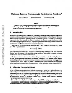
In this section, we demonstrate through numerical simulations that the discretized map (14) generates chaos, and that the global optimum can be found by applying the hybrid type of the chaotic annealing method to its trajectories. In this paper, we deal with the 5-cities TSP as an example. Cities are configured randomly in a 10 × 10 square, and their positions are shown in Table 1 and Fig.1. The globally optimal route which minimizes the total distance is 1 → 2 → 5 → 3 → 4, and the value of it is 26.63. Some locally optimal routes whose total distance are comparatively small are shown in Table 2.

We show the detail algorithm as follows, noting that we describe the generated states by the discretized map ˜ and candidates for the optimum as x. (14) as x

Table 1 Position of cities for the example. City No. x y 1 9.139 9.396 2 9.383 2.360 3 7.538 2.620 4 1.998 2.706 5 9.212 0.672

[The algorithm of the hybrid type of the chaotic annealing]

In this simulation, we use the values of the parameter in the objective function as A = 50.0 and B = 5.0. Regarding the sampling time ∆T in the discretized map (14) as a bifurcation parameter, we show the bifurcation

SICE02-0200 terms of their corresponding tempereture. The number of trajectories are 100, and their initial points are given randomly. We can see that trajectories converge into some points as ∆T → 0. The value of each component xik for some convergence points take 0 or 1 with little deviation, but there are other convergence points whose components take 0 < xik < 1 satisfying (1b), while (1c) is unsatisfied. Fig. 1 Position of cities for the example.

Table 2 Globally and locally optimal routes and their total distance. Optimal route Total distance 1→2→5→3→4 26.63 1→4→3→2→5 27.61 1→3→2→5→4 27.80 1→3→5→2→4 28.40 1→2→5→4→3 28.73

diagrams for each x11 through x55 in Fig.2. The initial point of trajectories is given as a certain value generated by random numbers normalized to satisfy (4b) and (4c). The bifurcation parameter varies from 0.0 to 0.2, and the states of trajectories generated from at 950th to 1000th time step are plotted for each value of ∆T . We can see that each component of the decision variable can change variously as ∆T gets large, which shows the chaotic characteristic.

Fig. 3 Result of applying the classical chaotic annealing to the map (14).

Then, we show the result for the application of the hybrid type of the chaotic annealing method to the TSP. The simulation conditions are, the initial temperature ∆T0 = 0.16, decrease of the temperature in one cooling d = ∆T0 /100, the threshold value T = 1.0, parameters for cooling schedule C1 = 10 and C2 = 20. Fig.4 is the plotting of all passing points for 100 trajectories of x(t). We can see that the cooling processes are definitely different between the classical method and the hybrid method. Moreover, in the hybrid case, the value of each component xik for all convergence points takes only 0 or 1.

Fig. 2 Bifurcation diagram of x for (14).

For the purpose of reference, we show the result for the application of the classical chaotic annealing method to the TSP. In the following simulation, we set the initial temperature ∆T0 = 0.16, and monotonuously decrease it by ∆T0 /100 = 1.6 × 10−3 after 20 transitions for each temperature while ∆T > 0. Fig.3 shows the plotting of all passing points for trajectories of x(t) in

Table 3 shows the convergence rate of trajectories to the global optimum and local optima. In the figure, “Classical” shows the rate when applying the classical chaotic annealing method, and “Hybrid” shows the rate when applying the hybrid type of the chaotic annealing method. It is clear that there is an outstanding difference of the optimization ability between the two annealing methods. In addition, the total rates of convergence to either of the best 5 local optima sum up to 67.4% in the hybrid method, but in the classical method only 4.7%.

SICE02-0200

References [1] H.Sugata and K.Shimizu, “Global Optimization Using Chaos in a Quasi-Steepest Descent Method”, IEICE Transactions (A), vol.J79-A, no.3, pp.658668, 1996 (in Japanese) [2] I.Tokuda, K.Onodera, R.Tokunaga, K.Aihara and T.Nagashima, “Global Bifurcation Scenario for Chaotic Annealing Dynamical System which Solves Optimization Problem and Analysis on Its Optimization Capability”, IEICE Transactions (A), vol.J80-A, No.6, pp.936-948, 1996 (in Japanese) Fig. 4 Result of applying the hybrid type of the chaotic annealing to the map (14).

Table 3 The convergence rate of trajectories to the optima Optimal route Classical Hybrid 1→2→5→3→4 2.5% 20.8% 1→4→3→2→5 0.1% 14.3% 1→3→2→5→4 0.3% 13.8% 1→3→5→2→4 0.6% 9.4% 1→2→5→4→3 1.2% 9.1%

6.

Conclusion

The chaotic optimization method gets increasing attention as an engineering application of the chaotic dynamical systems. A Map derived by discretizing the continuous dynamics of a gradient model generate chaos if its sampling time is set comparatively large, and the application of annealing methods to the map enables us to search the global optimum. While this method is shown to be efficient for optimization problems with lower and upper bounds, but we consider the application of it to the TSP, a special form of problems with normalized equalities and nonnegativies. By giving a state variable expression of the VMGP method which is applicable for this type of the problems, discreting it with Euler’s method, and combining the normalization of the output variable in order not to deviate normalized equalities due to the nonlinerity, we propose the discretized map of the VMGP method. The chaotic characteristic of the map is demonstrated, and the application of the chaotic optimization method to its trajectories is shown to be efficient for finding the global optimum by numerical simulations.

[3] Chang-song Zhou and Tian-lun Chen，“Chaotic annealing for optimization”，Phys.Rev.E，vol.55， No.3，pp.2580-2587，1997 [4] H.Ryota and E.Aiyoshi, “Variable Metric Gradient Projection Method and Replicator Equation”, 1999 IEEE Intl. Conf. on System, Man, and Cybernetics,III-515-520, 1999 [5] K.Masuda and E.Aiyoshi, “Global Optimization with Normalized Constaint using Chaos Mappings on a Simplex”, 29th SICE Symp. on Intelligent Systems, pp.23-28, 2002 (in Japanese) [6] M.Yamaguti and H.Matano, “Euler’s Finite Difference Scheme and Chaos”, Proc. Japan. Acad., vol.55(A), pp.78-80, 1979 [7] M.Hata, “Euler’s Finite Difference Scheme and Chaos in Rn ”, Proc. Japan. Acad., vol.58(A), pp.178-181, 1982 [8] K.Masuda and E.Aiyoshi, “Hybrid Type of Global Optimization Method with Discretized Chaos Mappings and Increase Accepting Methods”, Transactions of The Institute of Electrical Engeneers of Japan, vol.122-C, no.5, pp.892-899, 2002 (in Japanese)