Solving Boundary Value Problems With Neumann ...

World Applied Sciences Journal 20 (Mathematical Applications in Engineering): 129-133, 2012 ISSN 1818-4952 © IDOSI Publications, 2012 DOI: 10.5829/idosi.wasj.2012.20.mae.99937

Solving Boundary Value Problems With Neumann Conditions Using Direct Method 1

P.S. Phang, 1,2Z.A. Majid, 2M. Suleiman and 1F. Ismail 1

Department of Mathematics, Faculty Science, University Putra Malaysia, 43400 UPM Serdang, Selangor, Malaysia 2 Institute for Mathematical Research, University Putra Malaysia, 43400 UPM Serdang, Selangor, Malaysia Abstract: In this paper, the direct method is utilized for solving second order two-point boundary value problem of Neumann type. The method will obtain the solution of the second order boundary value problem directly without reducing it to to first order equations. The method will be implemented using variable step size via shooting technique adapted with the Newton method. Numerical results are given to compare the efficiency of the proposed method with the bvp4c from the Matlab solver. Key words: Direct method % Neumann type % Shooting technique INTRODUCTION

to solve second order boundary value problem and Yao [9] applied iterative method of nonlinear Neumann boundary value problems. Recently, Aly et al. [10] solved the two-point nonlinear boundary value problems with Neumann boundary conditions by using Adomian decomposition method. Besides that, Kierzenka and Shampine [11] introduced a boundary value problem solver based on residual control and the MATLAB which call bvp4c. The purpose of this paper is to establish a new algorithm for solving the linear and nonlinear second order two-point boundary value problem subjected to Neumann boundary condition directly. The approach for solving higher order ordinary differential equation directly has been suggested by Suleiman [12] and; Majid and Suleiman [13]. We will extend the direct method using variable step size from Majid and Suleiman [13] and adapted with shooting technique via Newton method to solve the boundary value problem.

Two-point boundary value problems have been widely arisen in modeling of chemical reactions, the boundary layer theory in fluid mechanic and heat power transmission theory. These problems can be presented in several types of boundary conditions: e.g. Dirichlet, Neumann and mixed. Dirichlet boundary condition is the common boundary condition and has been solved by several researchers such as Hamid et al. [1] and Mohamad [2]. Liu [3] studied on Neumann-type boundary value problems and Han and Wang [4] proved the existence of solutions to mixed two point boundary-value problem for impulsive differential equations by variational methods. Robin boundary condition is another type of boundary condition; it is a linear combination of Dirichlet and Neumann boundary conditions. We are concerned for solving the Neumann type boundary value problem. There are many analytical and numerical techniques available to solve boundary value problem with Neumann condition including several well-known methods, such as Adomian decomposition method, finite difference method and collocation method. Dehghan [5] approached the numerical solution of a non-local boundary value problem with Neumann’s boundary conditions by using finite difference method. Ramadan [6] and Liu et al. [7] solved the Neumann type boundary value problems by polynomial and nonpolynomial spline approach. Siraj-ul-Islam et al. [8] proposed the collocation method with the Haar wavelets

MATERIALS AND METHODS Consider the second order two-point boundary value problem of the form: y ′′ = f ( x , y , y′ ), a ≤ x ≤ b

(1)

Subject to the Neumann boundary conditions: y ′( a ) = α , y′ (b ) = β

Corresponding Author: Z.A. Majid, Institute for Mathematical Research, University Putra Malaysia, 43400 UPM Serdang, Selangor, Malaysia. E-mail: [email protected]

129

(2)

World Appl. Sci. J., 20 (Mathematical Applications in Engineering): 129-133, 2012 

yn +1 = yn + hyn′ + h 2  −

 −1+ 2 q + 4 r + 5 r ( r + q )    60 p ( p + q )( p + q + r )( p + q+ r +1) 



+  1+ 2( p + q + 2 r ) + 5( pr + qr + r 

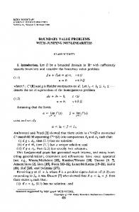
Fig. 1: Direct method variable step size



∫xnn+1 y′′( x) dx = ∫xnn+1 f ( x, y, y′) dx,



x x ∫xnn+1 ∫xn y′′( x ) dx dx = ∫xnn+1 ∫xn f ( x, y, y′) dx dx



n



(4)

y′′ = f ( x, y, y′ ) , a ≤ x ≤ b y ( a ) = sv ,

 −3+ 5q +10( r + qr + r 2 )  fn −3   60 p ( p + q )( p + q + r )( p + q + r +1)    

 



ϕ ( s) = y′(b, sv ) − β ≤ TOL

fn−2

2 + r + pr + 2 qr + r 2 )   60rq ( p + q)( r +1) 

f n −1

2 + 2 pr + 4 qr )   60 r ( q + r )( p + q + r ) 

 30( pqr + q 2 r + r 2 + pr 2 + r 3 + 2 qr 2 )   .   60r ( q + r )( p + q + r )    

sv +1 = sv −

(7)

ϕ ( sv ) . ϕ ′( sv )

(8)

Differentiate (6) with respect to s and it is simplify as follows:

fn

+ 2 pr + 4qr )   60(1+ r )(1+ q + r )( p + q + r +1) 

+  12 +15( p + 2q +3r ) p + 20( pq + q

(6)

We compute the {sv} by Newton method:

+  3+5( p + 2q +3r )+10( pq + q 

y′ ( a ) = α , v = 0,1,2,... .

We choose s0 = ($ – ") /(b – a) which is referring to Faires and Burden [14]. The stop condition for shooting technique is given as follow:

 

−  3+ 5( p+ 2q ) +10( pq + q

(5)

Implementation of the Method Shooting Technique: The shooting technique used to form the boundary value problem of Neumann boundary condition to initial value problems. The idea in shooting technique is to obtain the missing initial value until the boundary condition at the other end converges to its correct value. In order to correcting the guessing value, Newton method is adapted. Eq. (1) and (2) can be written by using shooting technique:

(3)

y′n +1 = yn′ + h  −



2 + 2 pr + 3r 2 )   60(1+ r )(1+ q + r )( p + q+ r +1) 

The direct method will solve boundary value problem of Neumann type adapted with shooting technique via Newton method.

The function f(x,y,y’) in (4) will be approximated using Lagrange interpolating polynomial, the value of yn+1 can be obtained by using MAPLE and the corrector formulae can be obtained as follows:

2)    

fn

  10(2 qr + pqr + q 2 r + pr 2 + r 3 + 2 qr 2 )   f n +1  .    60(1+ r )(1+ q + r )( p + q+ r +1)   

x

x yn +1 − yn − hyn′ = ∫x n+1 ( xn +1 − x ) f ( x, y, y′ ) dx

f n −1

+  2 +3( p + 2q + 3r ) p + 5( pq + q

yn′ +1 = yn′ + ∫x n+1 f ( x, y, y′ ) dx n

60 pq ( q + r )(q + r +1)

2 + pr + 2 qr + r 2 )   60 rq ( p + q)( r +1) 

 20( qr + pqr + q 2 r + pr 2 + r 3 + 2 qr 2 )   .   60 r ( q + r )( p + q + r )  

Let xn+1 = x + h, the Eq. (3) gives:



fn−2

 1+ 2( p + 2q + 3r ) + 5( pq + q 2 + 2 pr + 3r 2 )    60 r ( q + r )( p + q + r )  

x

+  3+5( p + q ) +10( r + pr + qr + r

)   

+ 

x

x

2

−  1+ 2( p + 2 q + 2 r ) + 5( pq + q

In Fig. 1 show that the approximated value yn+1 has the current step size, h and the previous step size were rh, qh and ph. The corrector formulae will involve the set of points {xn–3, xn–2, xn–1, xn, xn+1}, while the predictor formulae will involve the set of points {xn–3, xn–2, xn–1, xn,}. The corrector formulae of direct method were derived using Lagrange interpolation polynomial of order five and the predictor formulae were derived using the Lagrange interpolation polynomial of order four. We obtained the approximation values of yn+1 at the points x n+1by integrating once and twice over Eq. (1) with respect to x over the interval [xn, xn+1. x

60 pq ( q + r )(q + r +1)

fn −3

2

d d f ( x, y, y′) z + f ( x, y, y′) z ′, a ≤ x ≤ b dy dy′ z (a ) = 1, z′( a) = 0. z′′ =

  30( pqr + q 2 r + 2 r 2 + pr 2 + r 3 + 2 qr 2 )   f n +1  .    60(1+ r )(1+ q + r )( p + q+ r +1)   

130

(9)

World Appl. Sci. J., 20 (Mathematical Applications in Engineering): 129-133, 2012

Therefore, the solutions of (8) will gives n’(sv) = iz.(b,sv). The new guess can be calculated base on the previous guess using: sv +1 = sv −

y′ ( b, sv ) − β , z′ ( b, sv )

v = 1,2K

The successful step is dependent on the condition local truncation error (LTE) < TOL. If this condition fails, the values of the approximate solution, yn+1 are rejected and the current step size is reduce and recalculate the approximate solution.

(10)

Both of equations (6) and (9) will be solved simultaneously using the direct method. The process is repeated over and over until the error |$ – y’ (b,sv)| # TOL.

Algorithm of Direct Method Variable Step Size (DMVS) via Shooting Technique Adapted with Newton Method: Step 1 : Set Tol s0 Step 2 : Set x = x + h, evaluate yn+1 and zn+1 with direct method and compute fn+1 and znn+1. Step 3 : If x < b, repeat Step 2. If x = b, go to Step 4. Step 4 : If fulfill stop condition: |$ – y’(b,sv)| # Tol, go to Step 6. If not, go to Step 5. Step 5 : Generate the new guessing values by Eq. (9) and go to Step 2. Step 6 : Complete.

Variable Step Size Strategy: In order to reduce the computation time, the variable step size strategy will be implemented and this strategy is referring to Shampine and Gordon [15]. Three basic strategies are proposed for the step size adjustment, where the next step size will be restricted to half, double or the same as the current step size. The successful step size will remain constant for at least two blocks before we considered the next step size to be doubled. When a fail step occurs, the next step size will be halved of the previous step size. The following are some of the cases for choosing step size:

This algorithm was developed in C language. RESULTS AND DISCUSSION

Case 1: First time successful step: (p = q = r = 1). Substitute p = q = r = 1 in (5) will produce the following corrector formulae: h   yn′ +1 = yn′ −  −251 f n +1− 646 f n + 264 f n −1−106 f  n − 2 +19 f n − 3  720  h2 yn +1 = yn + hy′n − ( −135 f n +1 − 752 f n + 264 f n −1 −96 f n − 2 1440

In this section, four numerical examples are presented. These problems will be tested by the direct method with three different, Tol: 10G3 and 10G5. The numerical results will be comparing to the MATLAB solver, bvp4c for two different step sizes, h: 0.1 and 0.05. The MATLAB solver, bvp4c solves two point boundary value problems by collocation method. The following notations are used in the tables:

+17 f n − 3 )

Case 2: Second time successful step: (p = q = r = 1/2). Substitute p = q = r = 1/2 in (5) will produce the following corrector formulae:

h Tol MAXE AVE TFC TS IG FS bvp4c DMVS

h ( −269 f n +1 − 1360 f n + 1220 f n −1 − 615 f n − 2 900 +124 f n − 3 )

y′n +1 = yn′ −

h2 ( −129 f n +1 − 1430 f n + 1080 f n −1 1800 −525 f n − 2 + 104 f n − 3 )

yn +1 = yn + hyn′ −

Case 3: First time failure step: (p = q = r = 2). Substitute p = q = r = 2 in (5) will produce the following corrector formulae: h yn′ +1 = yn′ − ( −40192 f n +1 − 68005 f n + 10255 f n −1 100800 −3423 f n − 2 + 565 f n − 3 )

Step size Tolerance Maximum error Average error Total function call Total step at last iteration Total iteration of guess Failure step at last iteration MATLAB solver Direct method variable step size adapted with shooting technique via Newton method.

Problem 1: Linear boundary value problem: y ′′ = − y − 1, 0 ≤ x ≤ 1.

Neumann boundary condition:

h2 ( −13808 f n +1 − 42175 f n 100800 +4935 f n −1 − 1617 f n − 2 + 265 f n − 3 )

yn +1 = yn + hyn′ −

y ′(0) = (1 − cos(1)) / sin(1), y (1) = − (1 − cos(1)) / sin(1).

131

World Appl. Sci. J., 20 (Mathematical Applications in Engineering): 129-133, 2012 Table 1: Comparison bvp4c with DMVS for Problem 1

Exact Solution: 1 − cos(1) sin( x) − 1. sin(1)

y = cos( x) +

MAXE AVE TFC TS IG FS

Problem 2: Linear boundary value problem: y ′′ = − xy + (3 − x − x 2 + x 3 ) sin( x ) + 4 x cos( x ), 0 ≤ x ≤ 1.

bvp4c ---------------------h=0.1 h=0.05

DMVS -------------------------------------------Tol=e-3 Tol=e-5 Tol=e-7

6.4e-6 6.6e-6 117 -

2.5e-6 2.4e-6 63 26 2 0

6.2e-6 6.3e-6 227 -

8.7E-8 8.3E-8 79 34 3 0

2.6e-9 2.4e-9 102 42 3 0

Table 2: Comparison bvp4c with DMVS for Problem 2

Neumann boundary condition: y′(0) = −1, y′(1) = 2sin(1).


Exact Solution: y = sin 2 (π x ).

Problem 3: Non-linear boundary value problem:

bvp4c ---------------------h=0.1 h=0.05


1.7e-5 1.4e-5 110 -

3.2e-4 2.9e-4 64 26 2 0

1.5e-5 1.3e-5 210 -

2.3e-5 2.1e-5 84 34 2 0

3.8e-7 3.3e-7 125 50 2 0


y ′′ = y + 2π cos(2π x ) − sin (π x ), 0 ≤ x ≤ 1. 2

2

4

Neumann boundary condition:


y ′(0) = 0, y ′(1) = 0.

Exact Solution: 1 − cos(1) y = cos( x) + sin( x) − 1. sin(1)

bvp4c ---------------------h=0.1 h=0.05


1.0e+0 9.9e-1 220061 -

8.6e-4 1.1e-4 90 36 1 0

4.8e-4 4.4e-4 74129 -

7.0e-5 9.8e-6 124 49 1 0

1.5e-6 2.9e-7 210 83 1 0


Problem 4: Non-linear boundary value problem: MAXE AVE TFC TS IG FS

y′′ = − exp( −2 y ), 0 ≤ x ≤ 1.

Neumann boundary condition: 1 y′(0) = 1, y′(1) = . 2 Exact Solution:

bvp4c ---------------------h=0.1 h=0.05


2.5e-5 2.5e-5 202 -

3.9e-5 3.6e-5 65 27 6 0

1.5e-5 1.5e-5 382 -

4.7e-6 4.4e-6 85 36 6 0

2.5e-7 2.3e-7 123 52 7 0

DMVS at Tol = 10G3 and bvp4c at h=0.1 and h=0.05 are 2.54E-06, 6.37E-06 and 6.16E-06 respectively. As the tolerance getting smaller, the maximum error and average error for DMVS is better compare to bvp4c when Tol = 10G5 and 10G7. For example in Table 2 the average error for DMVS at Tol = 10G7 and bvp4c at h=0.05 are 3.26E-07 and 1.34E-05 respectively. For the non-linear boundary value problem, both methods managed to give the similar conclusion, e.g. in Table 3 and 4, the maximum error for DMVS at Tol = 10G7 and bvp4c at h=0.05 are 1.46E-06, 4.75E-04 and 2.51E-07,

y = ln(1 + x).

The numerical results of the bvp4c and DMVS to solve Problem 1-4 are presented in Tables 1-4 respectively. Firstly, we are interested to discuss the numerical results obtained by bvp4c with two different step size and DMVS at Tol = 10G3. The maximum error and average error for DMVS is comparable with bvp4c in most of the cases. For example in Table 1, the maximum error for 132

World Appl. Sci. J., 20 (Mathematical Applications in Engineering): 129-133, 2012

1.50E-05 respectively. We observed that the total function call for DMVS is less than bvp4c in all cases, this is expected because the DMVS solving boundary value problem directly with variable step size but bvp4c reduce the boundary value problem to the first order system equations and solve it using constant step size. For example in Table 3, the function call for DMVS is only 210 but bvp4c need 74129 function calls. As the tolerance getting smaller DMVS obtain better accuracy.

5.

6.

7.

CONCLUSION The main advantage of this paper is to apply the direct way of dealing with the second order boundary value problem. We have shown the proposed direct method with shooting technique using variable step size is suitable for solving second order linear and non-linear two-point boundary value problems with Neumann type. The numerical result shown that in term of accuracy, our proposed method can generate better accuracy even with less function calls.

8.

9.

10. ACKNOWLEDGEMENTS The authors gratefully acknowledged the financial support of Research University Grant Scheme (RUGS), No. project: 05-03-10-0973RU and sponsorship for MyBrain15 under Ministry of Higher Education.

11.

REFERENCES 1.

2.

3.

4.

Hamid, N.N.A., A.A. Majid and A.I.M. Ismail, 2011. Extended Cubic B-spline Method for Linear TwoPoint Boundary Value Problems. Sains Malaysiana, 40(11): 1285-1290. Mohamad, A.J., 2010. Solving second order nonlinear boundary value problems by four numerical methods. Eng. and Tech. Journal, 28(2): 369-381. Liu, Y., 2009. Studies on Neumann-type boundary value problems for second-order nonlinear p-Laplacian-like functional differential equations. Nonlinear Analysis: Real World Applications, 10: 333-344. Han, Z. and S. Wang, 2011. Mixed two-point boundary value problems for impulsive differential equations. Electronic Journal of Differential Equations, 35: 1-14.

12.

13.

14. 15.

133

Dehghan, M., 2003. Numerical solution of a non-local boundary value problem with Neumann’s boundary conditions. Commun. Numer. Meth. Engng, 19: 1-12. Ramadan, M.A., I.F. Lashien and W.K. Zahra, 2007. Polynomial and nonpolynomial spline approaches to the numerical solution of second order boundary value problems. Applied Mathematics and Computation, 184: 476-484. Liu, B.L., H.W. Liu and Y. Chen, 2011. Polynomial spline approach for solving second-order boundaryvalue problems with Neumann conditions. Applied Mathematics and Computation, 217: 6972-6882. Siraj-ul-Islam, Aziz, I. and B. Sarler, 2010. The numerical solution of second-order boundary-value problems by collocation method with the Haar wavelets. Mathematical and Computer Modelling, 52: 1577-1590. Yao, Q., 2010. Successively iterative method of nonlinear Neumann boundary value problems. Applied Mathematics and Computation, 217: 2301-2306. Aly, E.H., E. Abdelhalim and R. Randolph, 2011. Advances in the Adomian decomposition method for solving two-point nonlinear boundary value problems with Neumann boundary conditions. Computers and Mathematics with Applications, doi:10.1016/j.camwa.2011.12.010. Kierzenka, J. and L.F. Shampine, 2001. A BVP solver based on residual control and the MATLAB PSE. ACM Transactions on Mathematical Software, 27(3): 299-316. Suleiman, M.B., 1989. Solving nonsiff higher order ODEs directly by direct integration method. Applied Mathematics and Computation, 33: 197-219. Majid, Z.A. and M. Suleiman, 2006. Direct integreation implicit variable steps method for solving higher order systems of ordinary differential equations directly. Sains Malaysiana, 35: 63-68. Faires, D. and R.L. Burden, 1998. Numerical Analysis., USA: International Thomson Publishing Inc. Shampine, L.F. and M.K. Gordon, 1975. Computer Solution of Ordinary Differential Equations: The Initial Value Problem. San Francisco: W. H. Freeman and Company.