ESANN 2010 proceedings, European Symposium on Artificial Neural Networks - Computational Intelligence and Machine Learning. Bruges (Belgium), 28-30 ...
ESANN 2010 proceedings, European Symposium on Artificial Neural Networks - Computational Intelligence and Machine Learning. Bruges (Belgium), 28-30 April 2010, d-side publi., ISBN 2-930307-10-2.
Solving Large Regression Problems using an Ensemble of GPU-accelerated ELMs Mark van Heeswijk1 and Yoan Miche2 and Erkki Oja1 and Amaury Lendasse1 1 – Helsinki University of Technology - Dept. of Information and Computer Science Konemiehentie 2, 02015 HUT - Finland 2 – Institut National Polytechnique de Grenoble - Gipsa-Lab 961 rue de la Houille Blanche, F-38402 Grenoble Cedex - France
Abstract. This paper presents an approach that allows for performing regression on large data sets in reasonable time. The main component of the approach consists in speeding up the slowest operation of the used algorithm by running it on the Graphics Processing Unit (GPU) of the video card, instead of the processor (CPU). The experiments show a speedup of an order of magnitude by using the GPU, and competitive performance on the regression task. Furthermore, the presented approach lends itself for further parallelization, that has still to be investigated.
1
Introduction
Due to advances in technology, the size and dimensionality of data sets used in machine learning tasks has grown very large and they continue to grow by the day. Because of this, it is important to have efficient computational methods and algorithms that are able to deal with very large data sets, such that it is still possible to complete the machine learning tasks in reasonable time. Meanwhile, video cards are increasing more rapidly in terms of performance than typical desktop processors and they provide large amounts of computational power compared to typical desktop processors. For example, one of the most high-end video card at the moment, the NVidia GTX295, has 2 Graphics Processing Units (GPUs) which amount to a total of 1790 GFlops of computational power, compared to approximately 50 GFlops for a high-end Intel i7 Quad-core processor. With the introduction of NVidia CUDA [1] in 2007, it has become easier to use the GPU for general-purpose computation, since CUDA provides programming primitives that allow you to run your code on highly-parallel GPUs without needing to explicitly rewrite the algorithm in terms of video card operations. Examples of succesful applications of CUDA include examples from biotechnology, linear algebra [2], molecular dynamics simulations and machine learning [3]. Depending on the application, speedups of 10-300 times are possible by executing code on a single GPU instead of a typical CPU, and by using multiple GPUs it is possible to obtain even higher speedups. The introduction of CUDA has also lead to the development of numerous libraries that use the GPU in order to accelerate their execution by several orders of magnitude. An overview of software and libraries using CUDA can be found on [1].
309
ESANN 2010 proceedings, European Symposium on Artificial Neural Networks - Computational Intelligence and Machine Learning. Bruges (Belgium), 28-30 April 2010, d-side publi., ISBN 2-930307-10-2.
In this work, one of these libraries is used, namely CULA [4], which was introduced in October 2009 and provides GPU-accelerated LAPACK functions. Using this library the training of the models can be accelerated by an order of magnitude. The particular models used in this work are a type of feedforwardneural network, called Extreme Learning Machine (ELM) [5, 6]. The ELM is well-suited for regression on large data sets, since it is relatively fast compared to other methods and it has been shown to be a good approximator when it is trained with a large number of samples [7]. Even though ELMs are fast, there are several reasons to implement them on GPU and reduce their running time. First of all, because the ELMs are applied to large data sets the running time is still significant. Secondly, model structure selection needs to be performed (and thus multiple models with different structure need to be executed) in order to avoid under- and overfitting the data. Experiments are performed on two large regression data sets: the first one is the well-known Santa Fe Laser data set [8] for which the regression problem is based on a time series; the second one is steganalysis data [8]. The steganalysis data consist of data on a large number of images in which information has been embedded. The task is to estimate the amount of information that has been embedded in each image based on set of features extracted from that image. Section 2 discusses the models used in this work and how to select an appropriate model structure. Then an overview of the whole algorithm is given. Specifically, how multiple individual models are combined into an ensemble model and what parts are currently accelerated using GPU. Section 4 shows the results of using this approach on the two mentioned large data sets. Finally, the results are discussed and an overview of the work in progress is given.
2
Extreme Learning Machine for Large Dataset Regression
The problem of regression is about establishing a relationship between a set of output variables (continuous) yi ∈ R, 1 ≤ i ≤ M (single-output here) and another set of input variables xi = (x1i , . . . , xdi ) ∈ Rd . In the regression cases studied in the experiments, the number of samples M is large: 10000 for one case and 60000 for the second. 2.1
Extreme Learning Machine (ELM)
The ELM algorithm is proposed by Huang et al. in [5] and uses Single-Layer Feedforward Neural Networks (SLFN); the key idea of ELM is the random initialization of a SLFN weights. Consider a SLFN with N hidden neurons; in the case it perfectly approximates the data (meaning the error between the estimated output yˆi and the actual output yi is zero), it satisfies N +1 �
βi f (wi xj ) = yj , j ∈ �1, M �,
i=1
310
(1)
ESANN 2010 proceedings, European Symposium on Artificial Neural Networks - Computational Intelligence and Machine Learning. Bruges (Belgium), 28-30 April 2010, d-side publi., ISBN 2-930307-10-2.
with f the activation function, wi the input weights and βi the output weights. This writes compactly as Hβ = Y, with ⎞ ⎛ f (w1 x1 ) · · · f (wN x1 ) 1 ⎜ .. .. .. ⎟ , .. (2) H=⎝ . . . . ⎠ f (w1 xM )
···
f (wN xM ) 1
T T T with β = (β1T . . . βN +1 ) and Y = (y1 . . . yM ) . The output weights β can be computed from the hidden layer output matrix H and target values by using a Moore-Penrose generalized inverse of H, H† [9]. Overall, the ELM algorithm is then:
Algorithm 1 ELM Given a training set (xi , yi ) ∈ Rd × R, an activation function f and the number of hidden nodes N , 1: - Randomly assign input weights wi , i ∈ �1, N �; 2: - Calculate the hidden layer output matrix H; 3: - Calculate output weights matrix β = H† Y. The only parameter of the ELM algorithm is therefore the number of neurons to use in the SLFN. This is determined using an information criterion through model structure selection. 2.2
Model Structure Selection
Model structure selection enables to determine an optimal number of neurons for the ELM model. This is done using a specific criterion which estimates the model generalization capabilities for each different number of neurons; the classical Bayesian Information Criterion (BIC) [10, 11] has been used to select an appropriate number of neurons for an ELM model. The BIC is defined as
RSS + p × log M, (3) BIC = M × log M where RSS is the residual sum of squares, p the number of parameters of the model (number of neurons for ELM) and M the number of samples.
3
Parallel Implementation of ELM
In order to minimize data transfer times, the H matrix is computed once on an initially very large number of neurons using Eq. 2. It is then transfered fully to the memory of the graphics card and the BIC is computed for varying number of neurons. The minimization of the BIC enables to determine an optimal number of neurons for the ELM. Figure 1 summarizes the overall implementation. The parallelization possibilities appear clearly from this design.
311
ESANN 2010 proceedings, European Symposium on Artificial Neural Networks - Computational Intelligence and Machine Learning. Bruges (Belgium), 28-30 April 2010, d-side publi., ISBN 2-930307-10-2.
Training
Validation
X
ELM 1
ŷ1
X
ELM 2
ŷ2
α1 ≥ 0 α2 ≥ 0 α100 ≥ 0
X
ELM 100
minimizing validation error
∑
Y
ŷ100
Fig. 1: Block diagram of the parallel setup using ELMs. Since ELM are partially random non-linear models, they provide a set of quasi-independent models. For that reason, it is possible to use an ensemble methodology in order to achieve better generalization performance. The independence between the ELM is increased by using a random subset of variables for the training of each ELM. A total of 100 ELM models are build and a validation estimate of the output is computed on a validation set (subset of the original data set, only used for validation) for each model. These validation outputs (for the 100 ELMs) are used with the real output to solve the system with positivity constraints on the weights. This creates a linear combination with positive weights of the 100 ELM models. The obtained combination is then evaluated on a test set (also subset of the original data set). For the current version of our program and results presented here, only the solution of the system H is computed on the GPU [4], since it is the most time-consuming part of the ELM model construction. Furthermore, the 100 models built are created sequentially on the same GPU core. Section 5 discusses future improvements of the current setup.
4
Experiments and Results
Experiments are performed on two relatively large regression data sets: the first one is the full Santa Fe Laser data set [8] for which the regression problem is based on a time series; the second one is steganalysis data [8] (information has been embedded in a hidden manner in JPEG images and the amount of information is estimated through a set of features extracted from each image). Sizes of the data sets are given in Table 1: 75% is used for training, 10% for validation and 15% for test. The experiments have been repeated 10 times for the Santa Fe and the Steganalysis data. Table 2 gives the Normalized Mean Square Test Errors (NMSE) and the computational times for both CPU (on an Intel Core i7 920) and GPU
312
ESANN 2010 proceedings, European Symposium on Artificial Neural Networks - Computational Intelligence and Machine Learning. Bruges (Belgium), 28-30 April 2010, d-side publi., ISBN 2-930307-10-2.
Santa Fe Steganalysis
Total Size (samples×variables) 10081 × 12 60000 × 275
Training
Validation
Test
7561 45000
1008 6000
1512 9000
Table 1: Sizes of the used data sets. First column gives original total size of the data, while the other columns only mention the number of samples used in each type of set (training, validation, test). implementation. Computational times are given for one ELM model (including the model structure selection).
Santa Fe Steganalysis
NMSE (std) 2.9E-3 (7.2E-4) 3.9E-1 (1.2E-1)
GPU timing 3.2 41
CPU timing 33 309
Speedup 10.3 7.54
Table 2: Results for both data sets: Normalized Mean Square Test Error and standard deviation (in parenthesis), timing of one ELM execution for the GPU and CPU (in seconds), and speedup factor. It should be noted that the CPU implementation of the ELM algorithm is using Matlab. While it could be argued that a pure C code implementation might be more efficient, the current Matlab computations use highly tuned LAPACK and BLAS routines which would be similar to a C version. For comparison, a SVM built on a similar steganalysis data set using the same number of variables, but only 10000 samples, would require 600 days for both training and selection of the hyperparameters of the SVM using 10-fold cross-validation [11, 12].
5
Discussion and Future Work
The experiments show a speedup of an order of magnitude, by using the GPU to speed up the slowest part of the algorithm. Furthermore, the proposed approach is able to achieve results on the regression task comparable to other algorithms. Although in the experiments only a data set of 6 · 104 samples is used, the approach used can scale up to 2 · 105 samples on the currently used hardware (NVidia GTX295). Using a NVidia Tesla C1060 GPU with more memory, it would scale to a data set of approximately 106 samples. At the moment, some improvements are currently being implemented. Instead of just running the most time-consuming part of the algorithm on the GPU (i.e. solving the linear system to train the ELM), the entire ELM will run on the GPU. Furthermore, the parallelization of the algorithm across different GPUs is being implemented such that several ELMs can be evaluated in parallel. Finally, other models than the ELM (such as Reservoir Computing methods [13]) are considered to be implemented on the GPU to create an ensemble of models as in this paper.
313
ESANN 2010 proceedings, European Symposium on Artificial Neural Networks - Computational Intelligence and Machine Learning. Bruges (Belgium), 28-30 April 2010, d-side publi., ISBN 2-930307-10-2.
References [1] NVidia CUDA Zone: http://www.nvidia.com/object/cuda_home.html. [2] V. Volkov and J. W. Demmel. Benchmarking GPUs to tune dense linear algebra. In SC ’08: Proceedings of the 2008 ACM/IEEE SCI’08, pages 1–11, Piscataway, NJ, USA. IEEE Press. [3] B. Catanzaro, N. Sundaram, and K. Keutzer. Fast support vector machine training and classification on graphics processors. In Proceedings of the 25th International Conference on Machine Learning (ICML 2008), pages 104–111, Helsinki, Finland, 2008. [4] CULA (GPU-Accelerated LAPACK): http://www.culatools.com/. [5] G-B. Huang, Q-Y. Zhu, and C-K. Siew. Extreme learning machine: Theory and applications. Neurocomputing, 70(1-3):489 – 501, 2006. [6] M. van Heeswijk, Y. Miche, T. Lindh-Knuutila, P. Hilbers, T. Honkela, E. Oja, and A. Lendasse. Adaptive ensemble models of extreme learning machines for time series prediction. In 19th International Conf. on Artificial Neural Networks, Limassol, Cyprus, 9 2009. [7] G-B. Huang, L. Chen, and C-K. Siew. Universal approximation using incremental constructive feedforward networks with random hidden nodes. IEEE TNN, 17(4):879–892, 2006. [8] Santa Fe and Steganalysis data available at: http://www.cis.hut.fi/ projects/tsp/index.php?page=research&subpage=datasets. [9] C. R. Rao and S. K. Mitra. Generalized Inverse of Matrices and Its Applications. John Wiley & Sons Inc, January 1972. [10] G. Schwarz. Estimating the dimension of a model. Annals of Statistics, 6:461–464, 1978. [11] Y. Miche and A. Lendasse. A faster model selection criterion for OPELM and OP-KNN: Hannan-quinn criterion. In Michel Verleysen, editor, ESANN’09: European Symposium on Artificial Neural Networks, pages 177–182. d-side publications, April 22-24 2009. [12] Y. Miche, A. Sorjamaa, P. Bas, O. Simula, C. Jutten, and A. Lendasse. Op-elm: Optimally pruned extreme learning machine. IEEE Transactions on Neural Networks, 2009. DOI: 10.1109/TNN.2009.2036259. [13] D. Verstraeten, B. Schrauwen, M. D’Haene, and D. Stroobandt. An experimental unification of reservoir computing methods. Neural Networks, 20(3):391 – 403, 2007. Echo State Networks and Liquid State Machines.
314